University of Windsor University of Windsor
Scholarship at UWindsor
Scholarship at UWindsor
Electronic Theses and Dissertations Theses, Dissertations, and Major Papers
2009
PathAB: A New Method to Estimate End-to-End Available
PathAB: A New Method to Estimate End-to-End Available
Bandwidth of Network Path
Bandwidth of Network Path
Debashis Roy University of Windsor
Follow this and additional works at: https://scholar.uwindsor.ca/etd
Recommended Citation Recommended Citation
Roy, Debashis, "PathAB: A New Method to Estimate End-to-End Available Bandwidth of Network Path" (2009). Electronic Theses and Dissertations. 335.
https://scholar.uwindsor.ca/etd/335
This online database contains the full-text of PhD dissertations and Masters’ theses of University of Windsor students from 1954 forward. These documents are made available for personal study and research purposes only, in accordance with the Canadian Copyright Act and the Creative Commons license—CC BY-NC-ND (Attribution, Non-Commercial, No Derivative Works). Under this license, works must always be attributed to the copyright holder (original author), cannot be used for any commercial purposes, and may not be altered. Any other use would require the permission of the copyright holder. Students may inquire about withdrawing their dissertation and/or thesis from this database. For additional inquiries, please contact the repository administrator via email
PATHAB: A NEW METHOD TO ESTIMATE END-TO-END AVAILABLE BANDWIDTH OF NETWORK PATH
by
Debashis Roy
A Thesis
Submitted to the Faculty of Graduate Studies through the School of Computer Science in Partial Fulfillment of the Requirements for
the Degree of Master of Science at the University of Windsor
Windsor, Ontario, Canada
2009
PATHAB: A NEW METHOD TO ESTIMATE END-TO-END AVAILABLE
BANDWIDTH OF NETWORK PATH
By
Debashis Roy
APPROVED BY:
______________________________________________ Dr. K. Tepe
Department of Electrical Engineering
______________________________________________ Dr. R. Kent
School of Computer Science
______________________________________________ Dr. A. K. Aggarwal, Advisor
School of Computer Science
______________________________________________ Dr. S. Bandyopadhyay, Chair of Defense
School of Computer Science
iii
AUTHOR’S DECLARATION OF ORIGINALITY
I hereby certify that I am the sole author of this thesis and that no part of this thesis has been published or submitted for publication.
I certify that, to the best of my knowledge, my thesis does not infringe upon anyone’s copyright nor violate any proprietary rights and that any ideas, techniques, quotations, or any other material from the work of other people included in my thesis, published or otherwise, are fully acknowledged in accordance with the standard referencing practices. Furthermore, to the extent that I have included copyrighted material that surpasses the bounds of fair dealing within the meaning of the Canada Copyright Act, I certify that I have obtained a written permission from the copyright owner(s) to include such material(s) in my thesis and have included copies of such copyright clearances to my appendix.
iv ABSTRACT
v
DEDICATION
vi
ACKNOWLEDGEMENTS
First and foremost, I would like to express my sincere gratitude to my supervisor, Dr. Akshai Aggarwal, for always being a source of motivation and for giving me a definite direction to my research.
I would like to thank my committee members, Dr. Robert Kent and Dr. Kemal Tepe, for their valuable comments and suggestions towards my thesis. I would also like to thank Dr. S. Bandyopadhyay for being the chair in the examination committee.
vii
TABLE OF CONTENTS
AUTHOR’S DECLARATION OF ORIGINALITY ... iii
ABSTRACT ... iv
DEDICATION ...v
ACKNOWLEDGEMENTS ... vi
LIST OF TABLES ... xi
LIST OF FIGURES ... xii
1. INTRODUCTION ...1
1.1. Related Concepts ...2
1.1.1. Capacity ...2
1.1.2. Bottleneck Link & Bottleneck Bandwidth ...2
1.1.3. Utilization ...3
1.1.4. Available Bandwidth ...3
1.1.5. Tight Link ...4
1.1.6. Achievable Bandwidth ...4
1.1.7. Active and Passive Measurement ...4
1.1.8. Receiver-based vs. Sender-based Measurement ...5
1.2. Thesis Contribution ...7
2. SURVEY OF AVAILABLE BANDWIDTH ESTIMATE ALGORITHMS ...8
2.1. Gap-based Approach ...10
2.1.1. Cprobe ...11
2.1.2. Pipechar ...12
2.1.3. Spruce ...12
2.1.4. ab-probe ...13
2.1.5. PoTRI ...13
2.1.6. Summary ...14
2.2. Rate-based Approach ...15
viii
2.2.2. AB Estimate using Curve Matching ...17
2.2.3. Pathload ...18
2.2.4. PathChirp ...19
2.2.5. PathMon ...21
2.2.6. Pathtrait ...22
2.2.7. PoissonProb ...23
2.2.8. QuickProbe ...24
2.2.9. Algorithm proposed by Xiao et al. ...25
2.2.10.eChirp ...26
2.2.11.Summary ...27
2.3. Model-based approach ...29
2.3.1. Delphi ...29
2.3.2. IGI and PTR ...31
2.3.3. Stochastic queuing model ...33
2.3.4. Envelope ...34
2.3.5. Summary ...35
2.4. Probabilistic Approach ...36
2.4.1. SMART ...36
2.4.1.1. Probabilistic definition of Available Bandwidth ...36
2.4.1.2. The SMART algorithm ...37
2.4.2. A_ABE ...38
2.4.3. Summary ...40
2.5. Hybrid Approach ...40
2.5.1. BET ...41
2.5.2. MoSeab ...42
2.5.3. Summary ...43
2.6. Kalman Filtering based Algorithm ...44
2.6.1. BART ...45
2.6.2. Abest ...47
ix
3. THE PROPOSED ALGORITHM: PATHAB ...50
3.1. Client-Server Mode ...50
3.1.1. Initial Probing Phase ...51
3.1.2. Direct Probing Phase ...54
3.1.3. Complete client-server algorithm ...56
3.2. Stand-alone Mode ...57
3.2.1. Initial Probing Phase ...58
3.2.2. Direct Probing Phase ...59
3.2.3. Complete stand-alone mode algorithm ...59
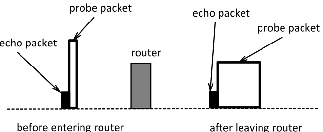
3.2.4. Position of the Echo Packet ...60
4. EXPERIMENT AND ANALYSIS ...62
4.1. Experiments using NS-2 simulator ...62
4.1.1. Single Tight-Link Scenario ...62
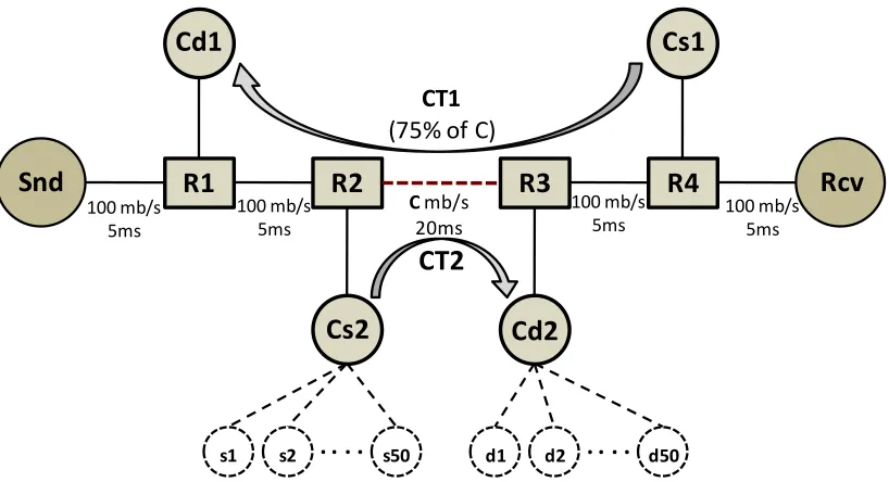
4.1.2. Multiple Tight Link: Pre and Post Bottleneck Cross-Traffic Effect ...69
4.1.2.1. Pre-bottleneck experiment ...70
4.1.2.2. Post-bottleneck experiment ...72
4.2. Experiments on Network TestBed ...74
4.2.1. Single-hop Experiments ...75
4.2.1.1. Description of Network TestBed ...75
4.2.1.2. Results of Single-hop Experiments ...76
4.2.2. Multi-hop Experiment: 10 Mbps range ...78
4.2.2.1. Description of Network TestBed ...78
4.2.2.2. Experimental Results ...79
4.2.3. Multi-hop Experiment: 100 Mbps range ...82
4.2.3.1. Description of Network TestBed ...82
4.2.3.2. Experimental Results ...83
4.3. Effect of Probe-Packet Size on Estimation Accuracy ...87
5. CONCLUSION AND RECOMMENDED FUTURE WORK ...89
REFERENCES ...91
APPENDIX A ...96
x
APPENDIX B ...99
B.1. Internet Control Message Protocol (ICMP) ...99
B.2. Use of ICMP packet in PathAB ...101
APPENDIX C ...103
C.1. E-mail communication with the authors of MoSeab ...103
xi
LIST OF TABLES
Table 2-1. Summary of Gap-based Algorithms ... 15
Table 2-2. Summary of Rate-based Algorithms ... 28
Table 2-3. Summary of Model-based Algorithms ... 36
Table 2-4. Summary of probabilistic algorithms ... 40
Table 2-5. Summary of hybrid algorithms ... 43
Table 2-6. Summary of Kalman filtering based algorithms ... 49
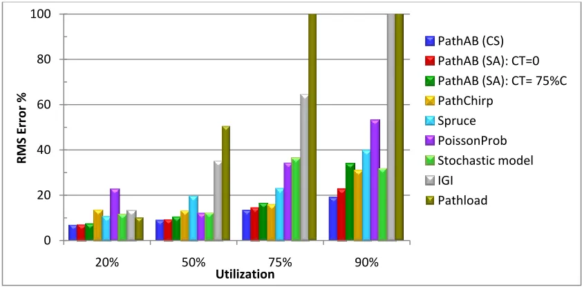
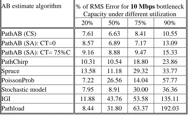
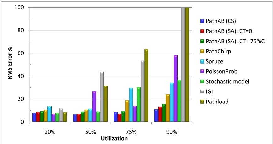
Table 4-1. RMS error % for 1.5 Mbps bottleneck Capacity under different utilization . 64 Table 4-2. RMS error % for 5 Mbps bottleneck Capacity under different utilization .... 65
Table 4-3. RMS error % for 10 Mbps bottleneck Capacity under different utilization .. 66
Table 4-4. RMS error % for 15 Mbps bottleneck Capacity under different utilization .. 67
Table 4-5. Average estimate of Available Bandwidth with Pre-Bottleneck Cross-traffic ... 71
Table 4-6. Average estimate of Available Bandwidth with Post-Bottleneck Cross-traffic ... 73
Table 4-7. Comparison of AB estimate algorithms for single-hop path with 10Mbps capacity ... 76
Table 4-8. RMS error % of pre-bottleneck experiments ... 79
Table 4-9. RMS error % of post-bottleneck experiments ... 81
Table 4-10. Average estimated AB by different algorithms in 100Mbps multi-hop path under pre-bottleneck traffic ... 83
Table 4-11. Average estimated AB by different algorithms in 100Mbps multi-hop path under post-bottleneck traffic ... 85
xii
LIST OF FIGURES
Figure 1-1. A pipe model with fluid traffic for four-hop network path ... 4
Figure 2-1. Gap-based Measurement ... 11
Figure 2-2. Offered bandwidth over measured bandwidth in TOPP for single-hop path ... 17
Figure 2-3. Sending curve Vs. Receiving curve ... 18
Figure 2-4. Exponentially distributed packets in PathChirp probe train ... 20
Figure 2-5. PathChirp queuing delay signature ... 20
Figure 2-6. Pathtrait train structure ... 22
Figure 2-7. eChirp train structure ... 26
Figure 2-8. Exponential flight pattern and its relationship with the MWM tree ... 30
Figure 2-9. Multifractal wavelet model (MWM) ... 30
Figure 2-10. Single-hop Gap Model ... 31
Figure 2-11. A probe-train [P1, …, Pn] of n packets enveloped by two packets E1k and E2k at router Rk ... 35
Figure 2-12. Modules of BET ... 41
Figure 2-13. Asymptotic relation between available bandwidth, probe traffic rate and expected inter-packet strain ... 46
Figure 2-14. Convergence of the BART method ... 47
Figure 2-15. Linear model of Abest ... 48
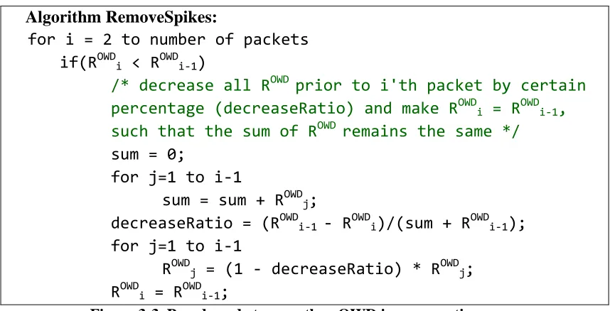
Figure 3-1. Exponentially spaced probing train ... 51
Figure 3-2. OWD Increase Ratio vs. Packet numner ... 52
Figure 3-3. Pseudo code to smoothen OWD increase ratio curve ... 53
Figure 3-4. OWD Increase Ratio vs. Packet numner (after removing spikes and fitting exponential curve) ... 54
xiii
Figure 3-6. Exponentially spaced probing packets with back-to-back echo packets ... 58
Figure 3-7. Packet distribution within a train in Stand-alone mode. Inter-packet gaps t1, t2, … , tN-1 are in Poisson distribution ... 59
Figure 3-8. Gap builds up between two packets if the echo packet is followed by probe packet ... 61
Figure 3-9. No gap builds up between two packets if the probe packet is followed by echo packet ... 61
Figure 4-1. Network model for single bottleneck experiments ... 63
Figure 4-2. RMS error % for 1.5 Mbps bottleneck Capacity under different utilization ... 65
Figure 4-3. RMS error % for 5 Mbps bottleneck Capacity under different utilization .. 66
Figure 4-4. RMS error % for 10 Mbps bottleneck Capacity under different utilization ... 67
Figure 4-5. RMS error % for 15 Mbps bottleneck Capacity under different utilization ... 68
Figure 4-6. Simulation topology for Pre-bottleneck and Post-bottleneck experiments .. 70
Figure 4-7. Average estimate of Available Bandwidth with Pre-Bottleneck Cross-traffic ... 72
Figure 4-8. Average estimate of Available Bandwidth with Post-Bottleneck Cross-traffic ... 74
Figure 4-9. Network topology for single-hop experiments ... 76
Figure 4-10. Comparison of AB estimate algorithms for single-hop path with 10Mbps capacity ... 77
Figure 4-11. Network topology for multi-hop experiments ... 78
Figure 4-12. Comparison of RMS error % for pre-bottleneck experiments ... 80
Figure 4-13. Comparison of RMS error % for post-bottleneck experiments ... 81
Figure 4-14. Comparison of average estimated AB by different algorithms in 100Mbps multi-hop path under pre-bottleneck traffic ... 84
xiv
Figure 4-16. Comparison of average estimated AB by different algorithms in
100Mbps multi-hop path under post-bottleneck traffic ... 86
Figure 4-17. Comparison of RMS Error % of estimated AB by different algorithms in 100Mbps multi-hop path under post-bottleneck traffic ... 86
Figure 4-18. Probe-packet size vs. Accuracy of estimation ... 88
Figure A-1. Non-homogeneous Poisson Process ... 96
1 CHAPTER I
1. INTRODUCTION
Network measurement techniques continue to receive a great deal of attention since networks are becoming an increasingly important part of today’s life. Numerous measurement tools and techniques have been developed to observe or monitor various network characteristics such as link capacity, available bandwidth, transmission delay, transmission loss and network topology etc. The results obtained from these tools have a number of applications in network management such as network troubleshooting, locating fault locations, network provisioning etc. Moreover with the ever increasing use of Internet in various applications, such as audio-video streaming, web applications, distributed database applications, mobile computing etc., estimating the available bandwidth of a network path has become more important. Knowledge of the available bandwidth of an end-to-end path can be used to enhance the performance and QoS of many network related applications, which require real-time traffic information to choose the best route for message transmission.
One important physical characteristic of a large network is the available bandwidth of a network path, which is defined as the maximum rate that the path can provide to a flow without affecting the rate of cross-traffic in the path. Knowledge of real time end-to-end available bandwidth has a variety of applications, such as, end-to-end flow control, in which hosts use end-to-end available bandwidth estimation to determine the rate at which they should transmit the data to avoid congestion in the network. Hosts can dynamically select the server with the highest potential available bandwidth for downloads and streaming media and determine whether the network has enough available bandwidth to meet the desired rate. In peer-to-peer networks, hosts use the available bandwidth information to select peers that can offer the best timely and efficient transfer of content. Network engineers and administrator use bandwidth estimations to troubleshoot networks, reroute network traffic and plan for future network expansions.
2
efficiently is a challenging task as the value of available bandwidth is highly dynamic in nature. The accuracy of measurement depends on the location of the bottleneck-link and the tight-link in the path, the cross-traffic rate of the path and several other factors. Moreover measurement methods have to take into account the complexity of network topologies, the diversity of traffic models and the probability of dropping measurement packets by the Intrusion Detection Systems (IDS).
1.1. Related Concepts
Before discussing the available bandwidth estimate techniques, it is necessary to clarify some terms and concepts that are very frequently used in network bandwidth related research. The most commonly used terms are explained in this section.
1.1.1. Capacity
Capacity is the maximum transmission rate at which a link can transmit data. It is a physical property of a link and thus does not change with time. A Link’s capacity or the maximum transmission rate of data through the link is mainly limited by two factors: the underlying physical transmission medium and the transmitter/receiver hardware. For a multi-hop network path, the link with minimum capacity determines the path capacity C.
1,2,...,
min i
i H
C C
(1.1)
where, Ci is the capacity of the i-th hop and H is the number of hops in the path.
1.1.2. Bottleneck Link & Bottleneck Bandwidth
3 1.1.3. Utilization
Utilization is the portion of capacity that is currently being used by cross-traffic on a hop or a path.
1.1.4. Available Bandwidth
Available bandwidth describes the portion of link capacity that is not being used by the network traffic. It can be obtained by subtracting utilization from capacity. It is the maximum rate at which data can be injected without affecting the cross-traffic. In a multi-hop path the link with minimum available bandwidth determines the available bandwidth of the path.
Let Ci be the link capacity of link i of an end-to-end path having H number of
hops. If λi(t) is the cross-traffic of link i at time t, then the available bandwidth Ai(t,T) of
link i is the average of unused bandwidth over some time interval T is given by:
1
( , ) T t( ( ))
i t i i
A t T C t dt
T
(1.2)Hence, the average available bandwidth of the path over the time interval T will be A(t,T), which is determined by the link with minimum available bandwidth, is:
1,2,...,
( , ) min i( , )
i H
A t T A t T
(1.3)
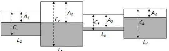
Figure 1-1 shows a pipe model with fluid traffic representation of a four-hop network path, where each link is represented by a rectangle. The height of each rectangle represents the capacity of the link and the height of shaded portion represents the amount of capacity used by the cross-traffic or the utilization. The height of un-shaded portion represents the available bandwidth of the link. In this example the minimum capacity C3
determines the end-to-end capacity and the minimum available bandwidth A4 determines
4
Figure 1-1. A pipe model with fluid traffic for four-hop network path
1.1.5. Tight Link
For a network path, the link with the least amount of available bandwidth is called the tight link. The available bandwidth of the tight link determines the path’s available bandwidth. The tight link of a network path may be different from the bottleneck link. In Figure 1-1 link L3 is the bottleneck link whereas link L4 is the tight link of the path.
1.1.6. Achievable Bandwidth
Achievable bandwidth is the maximum data transmission rate that an application can actually obtain over a network path. Achievable bandwidth depends on several factors such as, the available bandwidth of the path, the protocol and its implementation, the operating system(s) used, performance capability and the load of end hosts etc.
The difference between achievable bandwidth and available bandwidth is that, achievable bandwidth is an application metric that measures how much throughput an application can achieve, whereas available bandwidth is a physical layer metric that measures how much additional traffic can be injected into the path without interrupting the other network traffic.
1.1.7. Active and Passive Measurement
5
number of packets into the network to collect as many samples as possible to filter out the random behaviour of the network. Although passive measurements do not affect the network traffic, they are often less reliable than the active ones. Claffy and McCreary [1] showed that from passive measurements, it might not be possible to extract any useful data at all in some cases. Due to real time and accuracy requirements by most of the applications, available bandwidth estimation methods usually operate in the active mode.
1.1.8. Receiver-based vs. Sender-based Measurement
The active available bandwidth measurement tools can be divided into two categories: client-server based tools (also referred to as receiver based or double end-host tools) and stand-alone tools (also referred to as sender-based or single end-host tools). Typically client-server based tools must be installed in both source host and destination host of the network path; on the other hand stand-alone tools need to be installed only in the source host.
Generally the client-server based tool consists of two programs, the sender program which is installed in the source host and the receiver program or the server program which is installed on the destination host. During estimation process the sender transmits a series of packet-pairs or packet trains at different rates, while the receiver receives the probe packets and uses the timestamp information of all the packets to calculate the AB. It is impossible to deploy the receiver-based algorithm without the destination’s cooperation as it requires a server version of the estimation tool to be deployed at the destination. Users normally can install software in their own hosts, but they may not have administrative access to the destination host at the other end of the path. This may prevent the users from installing the receiver program on the destination host and hence may make available bandwidth estimation impossible.
6
The standalone available bandwidth estimation algorithms can have several network applications where the sender has limited access or no access to the receiver host. For example, currently several streaming media websites host video or audio in different qualities or bit-rates. The web-sites can decide about the quality and the associated bit-rate to be sent to a user, after determining the available bandwidth from the streaming media host to the user’s computer. As the web server may not have any access rights on a user’s computer, it may use standalone available bandwidth estimation algorithm to first estimate the AB of the path from web server to the user’s computer and then transmit the media of appropriate bit-rate so that the user can enjoy uninterrupted streaming media, without knowing any information about the network.
Almost all client-server based available bandwidth measurement algorithms are based on the following four basic assumptions:
All routers along the path follow first-in-first-out (FIFO) queuing The cross traffic follows the fluid model.
The cross traffic rate varies slowly and remains constant for the duration of available bandwidth estimation.
The sender host is able to inject probe packets at a rate higher than the available bandwidth.
In addition to the four, mentioned above, the standalone algorithms are based on three more assumptions:
The forward path from a sender to a receiver host and the returning path from the receiver to the sender host contain the same set of intermediate routers. The cross-traffic along the forward path determines the estimation result; the
cross-traffic along the reverse path has a negligible effect on the returning probe packets.
The receiver host can generate ICMP response packets.
7
to be installed at the receiving host. On the other hand standalone algorithms are easy to deploy as they do not require any tool to be deployed at the destination hosts. However most of the stand-alone methods are less accurate than the receiver-based methods.
1.2. Thesis Contribution
In the last two decades a great deal of research has been done on available bandwidth estimation of a network path and a considerable number of algorithms have been proposed. Most of these algorithms use active probing approach and operate only in the client-server mode. The algorithms have been developed based on different theoretical and mathematical foundations and assumptions. All the algorithms pose some advantages but with some drawbacks. For example, some algorithm may perform better on high link utilization but it may fail under low traffic scenario. This thesis first presents a comprehensive survey of existing available bandwidth measurement algorithms and then proposes a new available bandwidth estimation algorithm PathAB which has been developed combining the concepts used in three different methods and can operate both in client-server mode and in standalone mode.
8 CHAPTER II
2. SURVEY OF AVAILABLE BANDWIDTH ESTIMATE ALGORITHMS
All the existing available bandwidth measurement algorithms can be classified mainly in two categories: gap-based and rate-based algorithms. But because of different measurement approaches and network models used by different researchers in this survey the available bandwidth measurement algorithms have been divided into six categories. The six categories are: gap-based, rate-based, model-based, probabilistic, hybrid and Kalman filtering based approach.
Carter and Crovella [2] were the pioneer of available bandwidth measurement techniques. They introduced the first algorithm cprobe, a gap-based method, which estimates the available bandwidth based on the dispersion of long packet trains at the receiver. A similar approach is taken in pipechar [3]. Strauss et al. [4] introduce spruce
which focuses on measurement accuracy, failure patterns, probe overhead and implementation issues of bandwidth measurement techniques. Kazantzidis et al. [5] use a new sampling formula to sample the probing packets in algorithm ab-probe introduced by them. Xuan and Zheng [6] introduce a new available bandwidth measurement algorithm PoTRI, that uses tri-packet-probe instead of packet-pair used in all other gap-based technique.
Most of the researchers have preferred rate-based approach to estimate available bandwidth and proposed various rate-based available bandwidth measurement algorithms. Melander et al. [7] [8] propose the technique TOPP which addresses the hidden bottleneck problem in the network path. NEPRI [9] focuses on the macroscopic behaviour of the probing packet queued at the bottleneck link. He et al. [10] introduce a measurement method which uses a curve matching technique to estimate the available bandwidth. Jain and Drovolis [11] [12] propose a new rate-based measurement method “Self Loading of Periodic Streams” and implements this method in a tool called
Pathload. PathChirp [13] is based on the concept of “self-induced congestion” and uses exponentially spaced chirp probing train. The PathMon algorithm introduced by Kiwior
9
measurement to improve accuracy of estimate of the curve matching technique. Pathtrait
proposed in [15] uses three types of probing packets in the probing train and uses linear regression for bandwidth calculation. Xin [16] suggests a technique, PoissonProb, where the intervals between the probing packets are in Poisson distribution format. Kola and Vernon [17] propose a fast estimate method, QuickProbe, which calculates the available bandwidth in only two roundtrips with moderate accuracy. Xiao et al. [18] proposed a new algorithm which is based on Pathload’s concept but uses exponential search instead of binary search for fast estimate and compares the average interval difference of source and received trains, rather than comparing the rates. The eChirp algorithm introduced by Suthaharan and Kumar [19] uses the concept of exponential packet trains used in PathChirp but increases the inter-packet intervals by even powers. The algorithm combines three different sub-trains within a packet train to obtain more information about the network path.
Some researchers have used model-based approaches to measure available bandwidth. The Delphi algorithm [13] uses the multifractal wavelet model introduced by the same authors in an earlier paper [20]. Hu and Steenkiste [21] develop a single-hop gap model for the competing cross-traffic and based on this model they introduce two available bandwidth measurement algorithms, IGI and PTR. Kang et al. [22] introduced an algorithm based on a stochastic queuing model for single congested path. Bhati [23] extends the previous idea to design a recursive queuing model for multiple congested links and presents the algorithm envelope.
Almost all the algorithms fail to correctly estimate the available bandwidth when the network utilization is very low. To overcome this problem two groups of researchers proposed algorithms based on probability and statistics. Min et al. [24] proposed a new probabilistic definition of available bandwidth and based on this, they introduced the
10
new method A_ABE which dynamically uses NBE or IGI algorithm to estimate the available bandwidth.
Both gap-based and rate-based algorithms have some advantages as well as drawbacks which are described in section 2.5. To utilize the benefits of both of these approaches some researchers have proposed hybrid algorithms. Botta et al. [26] proposed a hybrid available bandwidth estimate tool called BET which integrates the three different concepts, the Packet Train Dispersion (PTD) technique of path capacity estimate methods, SLoEC (Self Loading Exponential Chirp) used by the PathChirp algorithm and the SLoPS (Self Loading of Periodic Streams) used by the Pathload algorithm. MoSeab
[27] on the other hand uses several probing train with increasing rate in the first phase (rate-based) to get a rough estimate of available bandwidth and in the next phase it uses a gap-based approach for final estimate.
BART [28] and Abest [29] are the only two algorithms which use Kalman filtering method to estimate the available bandwidth. The only difference between them is that BART algorithm transmits probe packets at a rate higher than the available bandwidth and hence overloads the path. Abest on the other hand sends probe packets at a lower rate than AB without congesting the network path.
The following section briefly describes the concepts and measurement approaches of each of these available bandwidth estimation algorithms.
2.1. Gap-based Approach
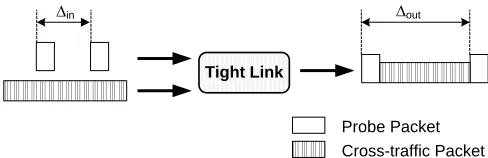
Gap-based algorithms are usually facilitated by packet pair/train properties. They use the information about the time gap between the arrivals of two successive probes at the receiver. “The advantage of this kind of algorithms is that they are very sensitive to the
burstiness of cross-traffic because of fine-grained interaction between the probing packets and cross-traffic packets” [16]. The main idea of gap-based approaches is that, if a pair of probe packet of size q is sent across a path of tight link capacity C with time gap Δin, such that Δin is not greater than q/C, then the cross-traffic packets will be queued up
11
when the packet pair reaches the receiver, the output time gap Δout will be greater than the
input time gap. Therefore, Δout is the time taken by the tight link to transmit the second
probe packet in the pair and the cross traffic that arrived during Δin as shown in Figure
2-1.
Tight Link
∆in ∆out
Probe Packet Cross-traffic Packet
Figure 2-1. Gap-based Measurement
Thus the time to transmit traffic is Δout −Δin, and the rate of cross traffic is, (Δout −Δin)/Δin ×C, where C is the capacity of the bottleneck. The available bandwidth is:
1 out in in
A C
(2.1)
Most of the gap-based methods make the following assumptions: (i) a single bottleneck link, (ii) the bottleneck link to be the tight link of the path and (iii) the router queue does not become empty between the departure of the first probe in the pair and the arrival of the second probe.
2.1.1. Cprobe
12
streams in order to tolerate packet drops and the possibility of re-ordering of packets. To eliminate some irregularities in the readings, cprobe discards the highest and the lowest inter-arrival measurements while calculating available bandwidth.
2.1.2. Pipechar
The algorithm Pipechar is proposed by Jin et al. [3] and it is implemented in the tool Network Characterization Services (NCS). It uses the same basic assumption about dispersion of long packet train like cprobe. The only difference is that pipechar can also operate in the passive mode through the deployment of NCS daemons on each subnet of the network infrastructure.
Though the algorithms cprobe and pipechar are straightforward, researchers are doubtful about some assumptions of these approaches. According to Dovrolis et al. [30]
“the dispersion of long packet train does not measure the available bandwidth in a path; instead, it measures a different throughput metric which is referred to as the asymptotic dispersion rate (ADR)”.
2.1.3. Spruce
Spruce [4] algorithm uses a series of packet-pairs to estimate available bandwidth. It assumes single bottleneck link and bottleneck capacity C to be known. Spruce uses 1500 byte probe packets and sets the intra-pair time gap Δin to the transmission time of a probe
packet on the bottleneck link. The main characteristic of spruce is that it sets the inter packet-pair gaps as Poisson distribution with an average which is much larger than Δin,
13 2.1.4. ab-probe
The ab-probe method was proposed by Kazantzidis et al. in [5]. Unlike existing gap-based methods, instead of calculating available bandwidth as the ratio of packet size and the inter-arrival time of two successive packets (referred to as “bytes over time”, BoT), the authors suggested a new sampling formula for the probe packets in ab-probe.
Ab-probe sends multiple streams of N packets each of size S at equal time intervals assuming that the packets reach the bottleneck link with input rate Pb. The available bandwidth for each stream is calculated using the following equation:
( 1)
( 1)
b
S P
C T N S
A C
N
(2.2)
Where, C is the bottleneck capacity and T is the observed time separation between the first packet and the N-th packet at the receiver. Ab-probe takes the average of the available bandwidths calculated for all the streams to estimate the available bandwidth of the path. The nettimer tool is used to measure the bottleneck bandwidth prior to ab-probe.
The authors state that they have tested their algorithm on both long range and short range internet connections using both packet-pairs and packet-trains method. They claim that ab-probe can successfully measure the available bandwidth in all cases, even for long distance network with more than 20 hops, whereas the existing BoT techniques may sometimes fail.
2.1.5. PoTRI
14
arrives which is a usual scenario for heavy cross traffic condition. The authors state that if a probe packet pair, with the second packet highly prioritized is transmitted-back to-back, when they arrive at the router, the second one will immediately go to the head of the service queue due to its high priority while the other one will wait at the end. Therefore the output gap of the two probe packets denote the waiting time in the queue. Based on this principle PoTRI sends three packets P1, P2 and P3 in each probe and the prioritized packet P2 is sent closely behind P1. The first two packets P1, P2 are used to measure the mean waiting time in the queue and the other two packets P1 and P3 are used to measure the mean transmission time from the difference of their output and input gaps. This information is then used to accurately calculate the overall utilization as well as the available bandwidth of the link.
According to the authors, PoTRI’s estimate for available bandwidth is quiet accurate for heavy cross traffic, but is unstable for low network utilization. Moreover, PoTRI needs the network facilities to support priority settings. If all routers in the network path do not support priority settings, the PoTRI becomes a usual probe gap method.
2.1.6. Summary
15
special requirement that all the routers of the path have to support priorities. Table 2-1 presents a summary of gap-based methods discussed in this section.
Table 2-1. Summary of Gap-based Algorithms
Algorithm Year Main Contribution/Feature Sender
Based
Cprobe [2] 1996 First algorithm to measure available bandwidth
Yes
Pipechar [3] 2001 Similar to cprobe but can operate both in
active and passive mode No
Spruce [4] 2003 Interval between the packet-pairs are set in Poisson distribution format
No
ab-probe [5] 2003 Use of packet trains instead of packet-pairs. Introduces a new available bandwidth sampling formula
No
PoTRI [6] 2006 Use of tri-packet-probe with a prioritized central packet to capture the effect of traffic packets queued at the router
No
2.2. Rate-based Approach
Most of the researchers have preferred rate-based approach to measure the available bandwidth of a network path. This type of algorithms are based on the concept of self-induced congestion: “If one sends probe traffic at a rate lower than the available
bandwidth along the path, then the arrival rate of probe traffic at the receiver will match their rate at the sender. In contrast, if the probe traffic is sent at a rate higher than the available bandwidth, then queues will build up inside the network and the probe traffic will be delayed. As a result, the probes‟ rate at the receiver will be less than their sending rate” [4]. Thus, the available bandwidth can be measured by searching for the turning point at which the probe sending and receiving rates start matching.
The advantage of rate-based algorithms is that they adapt widely to most of the network scenarios. They have better resistance to the cross-traffic effect and they can always report reasonable results. “In comparison to the rate-based algorithms, the
16
rate-based algorithm is that the network overhead to converge to the turning point is too high” [16].
2.2.1. TOPP
Melander et al. proposed the measurement methodology TOPP to estimate the available bandwidth of a network path [7, 8]. TOPP sends many packet pairs at gradually increasing probing rates from sender to the target host. Suppose that a packet pair, each packet having a size of L bytes, is transmitted through a link of capacity C with inter packet interval ; thus, the offered rate of the probing packet-pair will be RO=L/. If RO
is more than the end-to-end available bandwidth A, the link will become overloaded. Under this situation, if FCFS scheduling and random dropping of packets at buffer overflow is assumed, then the probe traffic will get a share of the link bandwidth proportional to the offered rate RO and this is measured by the receiver as Rm < RO. On
the other hand if RO < A, TOPP assumes that the packet pair will arrive at the receiver at
the same rate as it had at the sender (i.e., Rm = RO).
if
if
O O m O O O CR
R
A
R
R
C
R
A
R
R
(2.3)where, RC = C – A is the average cross-traffic rate of the link. Equation (2.3) can be re-written as:
1 if 1
1 if
O O O O m R A R A
R R A
R C C (2.4)
17
A
1
O
ff
e
re
d
/M
e
a
s
u
re
d
b
a
n
d
w
id
th
R
O
/R
m
Offered bandwidth RO
Figure 2-2. Offered bandwidth over measured bandwidth in TOPP for single-hop path
For a path consisting of multiple links, the RO/Rm curve may show multiple slope
changes due to queuing of probing packets at links having higher available bandwidth than A. To avoid this situation TOPP assumes that congested links are in Smallest Surplus First (SSF) order.
2.2.2. AB Estimate using Curve Matching
18
congestion point, it automatically shrinks the bandwidth range around the estimated congestion point and probes the network again.
0 5 10 15 20 25 30
1 2 3 4 5 6 7
Sending curve Receiving curve
Packet number
T
im
e
Figure 2-3. Sending curve Vs. Receiving curve
According to the authors this algorithm can calculate available bandwidth below 10Mbps with any desired accuracy. But for higher accuracy it requires more number of probing trains which increase the network overhead.
2.2.3. Pathload
Jain and Drovolis introduced the Pathload tool in [11] & [12]. Pathload uses Self-Loading Periodic Streams (SLoPS) to measure the available bandwidth. The basic idea of Pathload is that, if the stream rate R is greater than the available bandwidth A of the network path, the stream will cause a short term overload in the queue of the tight link. As a result the probe packets of the stream will queue up at the tight link and the One-way Delays of the probing packets will keep on increasing. On the other hand, if the stream rate is less than or equal to the path’s available bandwidth, the one-way delays of the packets do not change.
19
available bandwidth, Pathload gives a range (ABmin−ABmax) in which the Available Bandwidth belongs. It uses several probe streams to narrow down the range. Assume that the sender sends the n th probe stream with rate R(n). From the delay behavior of the received packets the receiver decides whether R(n)>A or not and informs the sender. The sender then estimates the rate of the next probing stream R(n+1) using the following method:
If, R(n) > A , Rmax = R(n) If, R(n) ≤ A , Rmin = R(n) R(n+1) = (Rmax + Rmin)/2
Initially Rmin is set to zero and R(n) & Rmax both are kept same and sufficiently large so that R(n) = Rmax > A. The algorithm terminates when (Rmax−Rmin)<ω, where ω is user defined estimate resolution. The algorithm needs log2 (R(0)) probing streams to converge.
The Pathload method assumes that there is zero packet loss at the bottleneck router, which means the router queue is large enough so that no cross-traffic packet is dropped during the probing. If this assumption is not satisfied, Pathload may underestimate the cross-traffic rate and over estimate the Available Bandwidth.
2.2.4. PathChirp
PathChirp is a novel available bandwidth estimate method introduced by Riberio et al. in [13]. Unlike all earlier measurement techniques it uses exponentially spaced probing packets in train to estimate path’s available bandwidth. The inter-packet gaps within a chirp decreases exponentially by a factor γ resulting in a rapid increase of probing rate within each train.
20
TgN2 Tg3 Tg2 Tg T 1 2 N-4 N-3 N-2 N-1 N
time
Probe packets
Figure 2-4. Exponentially distributed packets in PathChirp probe train
Queuing delay
Packet sending
time excursions
Figure 2-5. PathChirp queuing delay signature
The sender transmits M chirps each containing N exponentially separated packets. It first estimates per packet available bandwidth (Ek) for each packet k as follows:
i) Ek = Rk if k belongs to an excursion that terminates and qk ≤ qk+1
ii) Ek = Rl if k belongs to an excursion that does not terminate, where l is the start of the excursion
iii) Ek = Rl for all other cases
where, qk is the queuing delay and Rk is the instanteneous rate of k th packet in the train. It then takes a weighted average of all the Ek(m)’s to estimate per-chirp available
bandwidth D(m) using equation:
1 ( )
( ) 1
1 1
N m
k k
m k
N k k
E
D
(2.5)21
The main advantage of PathChirp is that to probe a network over the range of rates [G1, G2]Mbps it requires only log(G2) – log(G1) packets.
2.2.5. PathMon
PathMon is another algorithm, introduced by Kiwior et al. [14] to estimate available bandwidth, which follows almost similar curve matching technique inspired by the AB Estimation using Curve Matching method proposed by He in [10]. But to eliminate insignificant data and fluctuations of measurement, the algorithm first uses a single packet-train with a simple statistical evaluation.
The algorithm has two steps. In the first step, which is the jitter measurement step, PathMon sends one packet-train containing a series of Nj equally-spaced packets of the same size. The receiver collects the inter-arrival time gaps and uses statistical analysis to calculate the mean interval jitter, the standard deviation. It sends a large enough number of packets to obtain a good statistical sample of jitter.
In the second step, the algorithm sends a series of equal-sized packets, but with decreasing time interval, so that the instantaneous bandwidths of the packets are in increasing order and equally spaced between the lower and upper bounds of available bandwidth. The receiver records the receiving times of the packets in terms of cumulative time. PathMon calculates the available bandwidth by identifying the congestion point, i.e., the point of divergence between the inter-packet delays measured at the sender and the receiver.
22 2.2.6. Pathtrait
The Pathtrait method introduced in [15] can accurately locate the tight link and estimate the end-to-end available bandwidth of a network path. The method is based on a novel probing technique that uses three different types of probing packets in the probing train.
According to the authors, pathtrait technique is based on the assumptions that all the routers along the path follow FIFO queuing and generate ICMP packets and the cross traffic along the path follows a fluid model. Pathtrait uses three different types of packets, the Type-I packet can successfully reach the destination from the origin, Type-II packets are hop limited by setting a lower value for the TTL so that it is dropped at an intermediate router and Type-III packet which is hop limited ICMP packet that can generate ICMP response from an intermediate router. Pathtrait train consists of large load packets (Type-II) of size 1000 bytes, each of which is followed back to back by one backward packet (Type-III) or one forward packet (Type-I) of size 40 bytes alternatively. The Type-I packets are used to estimate the forward rate or output rate of a hop and Types-III packets are used to estimate the input rate or backward rate for the hop.
Load Packet (Type-II)
Forward Packet (Type-I)
Backward Packet (Type-III) time
Figure 2-6. Pathtrait train structure
23
estimate the available bandwidth. In this step it probes the network path with 15 trains with different rates calculated as:
(1 (8 ) )
i
R i
R (2.6)where, R is probing rate used in locating the tight link, Ri is the rate of i-th probing train and the value of ε is set to 2%. After obtaining the receiving rates of all the trains, it uses linear regression to solve (2.7) in order to obtain tight link bandwidth Ct and cross traffic rate .
1
if 1
1 1
if
I I
O
I t t I
R A
R
R
R A
C C R
(2.7)
where, RI are RO are the input and output rate respectively. Finally pathtrait calculates the
available bandwidth A of the path as Ct−.
The authors state that they have verified Pathtrait estimate using NS2 simulation environments and found that this method accurately identifies the tight link location in both constant cross traffic environment and in bursty environment. However the available bandwidth estimate is less accurate in bursty traffic condition.
2.2.7. PoissonProb
The PoissonProb algorithm was introduced by Xin in [16]. The algorithm was designed based on the study in [31] that, current network traffic on the internet follows Poisson distribution. The key concept of this method is that in a probe stream, the intervals between probe packets are in Poisson distribution format.
24
to estimate the bottleneck capacity of the path using histogram analysis of the timestamp information of the packets. In the next phase the client sends a train of Poisson distributed packets with mean inter-packet interval λ, set to 1/3 of the bottleneck separation gap. At the receiver, the average destination gap of the packets within a probing train is compared with the average source gap. If both gaps are the same ((source gap-destination gap)/destination gap ≤ 0.15), PoissonProb stops measurement and reports available bandwidth based on the probing rate of that train. Otherwise, it increases or decreases the value of λ by a factor of 1/5 and proceeds with the next round of measurement.
In the stand-alone or sender-based mode, PoissonProb requires only a UDP session between the sender and the receiver and sends UDP echo packets in Poisson distribution. The algorithm assumes that the packets are echoed back through the same route without being affected by the cross-traffic. The measurement strategy is similar to the client-server mode. The sending host observes the total initial gaps and the total gaps of the echo packets and stops measurement on reaching the turning point.
The main assumption of PoissonProb algorithm is that the network traffic pattern follows Poisson process. If the traffic pattern changes, this method fails to estimate the available bandwidth correctly.
2.2.8. QuickProbe
Kola and Vernon [17] introduced a rapid available bandwidth measurement technique, QuickProbe, which can estimate the available bandwidth in only two roundtrips. QuickProbe uses 19 probe packets on the first roundtrip to get a conservative estimate of the available bandwidth and then another 9-17 packets on the second roundtrip to refine the estimate.
25
rate feasibility results to determine the next probe rate in order to perform a binary search for the maximum feasible transmission rate, which is reported as the available bandwidth, similar to the Pathload approach. The key difference is that QuickProbe uses trains of 9 packets (or 17 packets if the probe rate is more than 100 Mbps) unlike 100 packets per train in Pathload. This significantly reduces the traffic overload and estimation time. According to the authors, QuickProbe may underestimate the available bandwidth in some cases due to the granularity of binary search.
2.2.9. Algorithm proposed by Xiao et al.
Xiao et al. [18] proposed a new available bandwidth measurement method which is based on the Self-Loading of Periodic Stream (SLoPS) concept introduced in Pathload [11]. Instead of comparing the received probe rate with the sending rate the proposed method uses a new technique, called interval difference, to infer the congestion. Also unlike Pathload instead of only using binary search method, it first performs an exponential search to quickly find the rough range and then performs binary search to search for the actual range of available bandwidth.
In each probing train the method transmits m2+1 probe packets of size L=100 bytes, where m is any integer. At the receiver the m2 received intervals are separated into
m groups. For example, the i-th group is {Om×i, Om×i+1, … , Om×i+m−1} whose average is
Oia, where 0 ≤ i < m and Ok is the received gap between k-th and (k+1)th packet. For each
train, the value of a parameter δ is calculated using the following formula:
1
0 ( ) , ( ) 1 , 0 ,
m a
i s i
a i s
F X O
F X
m O
(2.8)where, s=L/R, R is the sending rate, s is the sending interval and r is the estimated receiving interval of the probing train. If δ≤0.2 the algorithm reports s=r otherwise s<r.
26
difference between s and r is estimated. The rate of (n+1)-th probing train R(n+1) is calculated as:
If, s<r , Rmax = R(n) If, s=r , Rmin = R(n)
R(n+1) = R(n) ×2n
Once Rmax−Rmin reaches a threshold value the algorithms enters into the second phase and obtains a finer range of available bandwidth using binary search method similar to Pathload’s approach. Once the difference between Rmax and Rmin reaches the desired accuracy the algorithm reports the available bandwidth as A=(Rmax+Rmin)/2.
The authors state that the proposed algorithm requires smaller number of probing packets, it has less estimation time compared to Pathload and the estimate is more accurate.
2.2.10.eChirp
Suthaharan and Kumar [19] introduced a new available bandwidth estimation algorithm eChirp which has the same basic concept as the exponential packet train used in PathChirp, but uses a modified train structure. In the modified train structure (Figure 2-7) every odd packet repeats the probing structure and inter-packet gap as the previous packet. Moreover the probing rate is increased exponentially with only even power. The advantage of this type of train structure is that it requires half the number of probe packets within a chirp train as compared to PathChirp.
T T Ta2 Ta2 Ta4 Ta4
Ta2N-4 Ta2N-2
2T 2Ta2
2Ta4
T(a2+1) Ta2(a2+1)
Ta2N-4(a2+1)
2Ta2N-4 Ta2N-4
Figure 2-7. eChirp train structure
27
2 2 2 4 2 4 2 2
, , , , , , ,
N N N
Ta Ta Ta Ta Ta T T
The second train is spaced by the probing rate increase of:
2 4 2 2 6 2 2 2 2
( 1), ( 1), , ( 1), ( 1)
N N
Ta a Ta a Ta a T a
The third train is spaced by the probing rate increase of:
2 4 2 6 2
2Ta N , 2Ta N , , 2Ta , 2T
Hence the eChirp method can obtain more data than PathChirp to characterize the delay and excursion segmentation.
As each packet of the train belongs to three different sub-trains, each packet has three different instantaneous probing rate as well as per packet available bandwidth (
E
k jm, ) associated with it. The overall per packet available bandwidth for the train is calculated as a linear combination of per-packet available bandwidths of three sub-trains as:
3 ,1 ,2 ,3
/ 5m m m m
k k k k
E E E E (2.9)
where, m is the train number, k is the packet number j is the sub-train number which can have a value of either 1, 2 or 3 indicating whether the packet belongs to first, second or third sub-train. Because of the equal spacing between two consecutive packets, the per-chirp available bandwidth for a per-chirp train is calculated as:
1
2
m m
k k k
m
k
E E
D
(2.10)Finally the available bandwidth of the path is estimated as the average of all per-chirp available bandwidths.
2.2.11.Summary
28
overload the network path. This makes these methods much more intrusive compared to the gap-based algorithms. To overcome this problem, many researchers have focused on restructuring the packet trains to keep the probing rate and number of probe-packets as low as possible and gather more information about the network. Table 2-2 presents a summary of rate-based algorithms discussed in this section.
Table 2-2. Summary of Rate-based Algorithms
Algorithm Year Main Contribution/Feature Sender
Based TOPP [7, 8] 2000 Assumes proportional share of probe-traffic and
cross-traffic at the tight link. Uses trains of packet-pairs with linearly increasing input rate for the trains.
No
Curve Matching Algorithm [10]
2001 Uses curve matching technique to analyze the sending and receiving time curves of the probing packets.
Yes Pathload [11, 12] 2002 Self-adaptive method that estimates the range of
available bandwidth. Uses binary-search-like method to find out a range within which the actual AB may fall.
No
PathChirp [13] 2003 Usees exponentially spaced probing packets within a train. Requires only log(G2) – log(G1) packets to probe a network over the range of rates [G1, G2]Mbps.
No
PathMon [14] 2004 Similar to the Curve Matching Algorithm [10] but, calculates the mean inter-arrival jitter and standard deviation prior to bandwidth estimate to improve accuracy
No
Pathtrait [15] 2005 Uses three different types of probing packets (load packet, forward packet & backward echo packet).
No
PoissonProb [16] 2005 Intervals between the probe packets are in Poisson distribution format
Yes QuickProbe [17] 2006 Estimates available bandwidth with only two
roundtrips.
No Algorithm
proposed by Xiao
et al. [18]
2007 It is based on the SLoPS concept used in Pathload, but instead of only using binary search method, it first performs an exponential search to quickly find the rough range and then performs binary search to search for the actual range of available bandwidth.
No
eChirp [20] 2008 Instantaneous rates of even packets are increased exponentially with only even power and every odd packet repeats previous inter-packet gap. Each train consists of three sub-trains, which leads to more samples than PathChirp using less number of packets.
29 2.3. Model-based approach
This class of the available bandwidth measurement algorithms has been developed on the basis of the network traffic modeling research.
2.3.1. Delphi
The foundation of the Delphi algorithm [20] is based on the multifractal wavelet model
(MWM). The core idea of the MWM is that the cross-traffic stream is a superposition of many data flows that share common link resources with the probe connections. The statistical analysis showed that such superposition has the characteristics of self-similarity, burstiness, long-range dependence (LRD) and even multifractal behavior (non-Gaussianity) [32]. This multifractal behavior makes it possible to present aggregated cross-traffic as a binary tree structure. In this structure, the β multiplier splits parent aggregate into two child aggregates at the next scale which increases or decreases β flow of traffic. The MWM also provides means to estimate the queuing behavior of a synthetic trace through the Multiscale Queuing Formula (MSQ) [32].
30
Delphi estimates the total cross-traffic arriving in the interval T0 by recursive estimates of
cross-traffics in the intervals T1, T2 and so on.
Figure 2-8. Exponential flight pattern and its relationship with the MWM tree
Figure 2-9. Multifractal wavelet model (MWM)
(a) Binary tree structure of aggregated traffic. (b) Beta multipliers split parent aggregate into two child aggregates at the next finer scale
31 2.3.2. IGI and PTR
Hu and Steenkiste [21] presented a single-hop gap model to establish the relationship between the competing traffic throughput and the change of packet pair gap for a single-hop network. The model can be represented as a 3-D graph as shown in Figure 2-10. It shows the output gap gO as a function of the queue size Q and the competing traffic throughput BC.
BO*gI(1-r)
BC
JQR
Q 0
gB
gI DQR
gO
Figure 2-10. Single-hop Gap Model
Here, gB is bottleneck separation gap, gI is input gap between two packets P1 &
P2 of a pair, gO is output gap at the receiver, BO is bottleneck capacity, BC is cross-traffic
rate, Q is queue size when the first packet P1 of the pair arrives at the router and r=gB/gI
32 O I O Q g g B
(2.11)
On the other hand in JQR the output gap will have a linear relationship with competing traffic and can be represented by the following equation:
C I O B O B g g g B
(2.12)
Based on this model the authors proposed two available bandwidth estimation techniques, the gap-based method Initial Gap Increasing (IGI) and the rate-based method
Packet Transmission Rate (PTR). Both IGI and PTR algorithms send a sequence of packet trains with increasing input gap. The measurement process terminates when average output gap is the same as the average input gap. The input gap is kept sufficiently small to ensure that all the probe packets within a train fall in the joint queuing region. Now in the probing train, consider that M probing gaps are increased, K are unchanged and N are decreased. The IGI algorithm then calculates the available bandwidth as,
1
1 1 1
1
M
i B
i
M K N
i i i
i i i
O
g g
g g g
A B
(2.13)Here, the gap values G+ = {gi+ | i = 1, …, M}, G= = { gi= | i = 1, …, K }, and G− = {gi+ | i = 1, …, N}. BO Mi1
gi gB
is the amount of competing traffic that arrives at thebottleneck router during the probing period.
1 1 1
M K N
i i i
i g i g i g
is the totalprobing time.
The PTR algorithm on the other hand calculates available bandwidth using the equation,
1 1 1
M K N
i i i
i g i g i g
M K N L
(2.14)33 2.3.3. Stochastic queuing model
Kang et al. [22] presented a generic stochastic queuing model of an internet router. The model assumes that the router introduces random delay noise ω to each arriving probe packet because of the cross-traffic. If the probing train consists of n equal sized packets of size q then the departure times dn of the packets can be expressed as,
1 1
1
1
max( , ) 2
n
n n n
a n
d
a d n
(2.15)
Here, an is the arrival time of n-th packet and = q/C is the process time of a packet by the router of capacity C.
The main idea of the model is to transmit the packets with inter-packet interval x
in a way so that packet i arrives at the router before the departure time of packet i−1. This condition leads to an ≤ dn−1 and hence the inter-departure times yn of the packets after the bottleneck router are given by:
1 , 2
n n n n
y d d n (2.16)
In real networks such as the Internet, cross-traffic is bursty with a time-varying arrival rate. Considering the time varying nature of cross-traffic, the authors derive the mean output dispersion under arbitrary cross-traffic when the input spacing x ≤ q/C as:
[ ] xr
E y
C
(2.17)
where, r is the time-average of a cross-traffic arrival rate process r(t) at the tight link:
0 1 lim t ( )
t
r r u du
t
(2.18)Another important result in [22] shows that the variance of y decays to 0 as the packet-train length n (i.e., the number of packets in each train) increases. To estimate both capacity C and available bandwidth A from E[y], the paper [22] defines Wna and
b n