Formation and development of shear bands in granular material

Formation and Development of Shear Bands in

Granular Material

by

Michael Shearer, 1

F. Xabier Garaizar 2

Department of Mathematics North Carolina State University

Raleigh, NC 27695

David G. Schaeer 3

and John Trangenstein 4

Department of Mathematics Duke University Durham, NC 27706

Abstract

A system of equations modeling antiplane shear in a granular material is considered. The model includes the possibility of localization of strain, and the subsequent development of shear bands. This behavior is captured in our analysis of the Riemann initial value problem, in which an initial discontinuity propagates as a combination of moving waves and a stationary shear band. The analysis is veried by numerical results obtained with a Godunov method including adaptive mesh renement.

1. Introduction

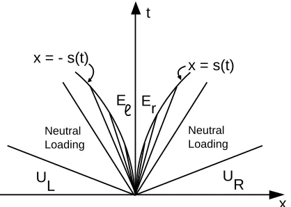
We consider a model [4] for dynamic deformations of granular materials which allows for the localization of ow and the consequent development of shear bands. We focus on Riemann initial value problems in one space dimension that include a shear band. An unusual feature of the solutions is that they are not scale invariant. The overall structure of the solution (shown in Figure 1) is that the material unloads elastically between the shear band and a free boundary that propagates into a region of plastic deformation. Mathematically, the Riemann problem reduces to solving a free boundary problem for the (linear) wave equation. We summarize short time existence results and long time behavior, the details of which are given in a series of papers [5, 2]. Then we outline the governing principles in designing an ecient numerical simulation

1Research supported by NSF grant DMS 9201115, which includes funds from AFOSR, and by ARO grant

DAAL03-91-G-0122.

2Research supported by NSF grant DMS 9201115, which includes funds from AFOSR. 3Research supported by NSF grant DMS 8804592, which includes funds from AFOSR.

4Research supported by NSF grant SES-DMS-9201361, by DNA grant DNA001-92-C-0166, and by DOE grant

DE-FG05-92ER25145

code, and present numerical results. The numerical results are in excellent agreement with the predictions of the analysis. The simulation code is designed so that it can generalize to higher dimensions.

The following system of equations describes antiplane shear deformations that depend on one space variablex and timet [4].

@ t

v =@ x

(a)

h

I+ 1 h()(

R T)T T

i @

t

T =c 2

@ x

v

0

!

(if loading) (b)

@ t

T =c 2

@ x

v

0

!

(if unloading): (c)

(1.1)

The dependent variablesvandT = (;)

T represent velocity and stress respectively, all other

entries of the full stress tensor being constant. T

T is the transpose of

T. The constant c is the

elastic wave speed, I is the 22 identity matrix and R is the rotation matrix

R =

cos sin ?sin cos

!

(1.2) with parameter 2(0;

2) measuring the degree of nonassociativity in the model (specically in

the ow rule). The given function h = h() is the hardening modulus, depending on the yield

stress . h is a nonnegative monotonically decreasing function on [0,1] withh(1) = 0.

Equation (1.1a) is conservation of momentum, while equations (1.1b,c) specify constitutive behavior. This behavior is described as loading (or plastic) when jTj is at its maximum over

previous time and is increasing. I.e., the material is loading when it is at plastic yield:

jT(x;t)j=(x;t) max 0st

jT(x;s)j; (1.3)

and the right hand side of (1.3) is increasing:

@ t

>0: (1.4)

Otherwise, the material behavior is said to be unloading (or elastic). We have a dierential equation for :

@ t

= (

@ t

jTj if loading

0 if unloading (1.5)

The Riemann problem for system (1.1) is the initial value problem with initial data of the form

(v;T;)(x;0) = (

(v L

;T L

; L) if

x<0

(v R

;T R

; R) if

x>0;

(1.6) subject to jT(x;0)j (x;0): In solving Riemann problems for a simplied version of system

is that equations (1.1) lose hyperbolicity as approaches = 1; and the classical construction

of scale invariant solutions breaks down.

When the equations lose hyperbolicity, they also lose linear well-posedness, and we suppose that a shear band forms. As in [4], we treat the shear band as a stationary discontinuity, with nonstandard jump conditions. Specically, the velocity gradient is approximated by a divided dierence:

v x

[v]=; (1.7)

where [v] is the jump in velocity across the shear band and is a small parameter measuring the

thickness of the shear band. From the conservation of momentum equation (1.1a), we see that

is continuous across a shear band. The variable experiences a jump on each side of the shear

band. The approximation (1.7) leads to the following system of ordinary dierential equations, with a constraint, for evolution of the variables T = (;)

T

; within the shear band.

h

I+ 1 h()(

R T)T T

i @

t

T =c 2 [

v]=

0

!

; =jTj: (1.8)

Note that these equations are coupled to the external variables through the jump [v] in v,

and through the continuity of: This system of equations may be regarded as a jump condition

for stationary shocks, analogous to the usual Rankine-Hugoniot condition for shocks. However, the Rankine-Hugoniot condition is a system of algebraic equations, in contrast to (1.8), which is a system of dierential equations. The jump condition (1.8) eectively widens the class of weak solutions of equations (1.1) beyond the class of solutions whose jump discontinuities satisfy the usual Rankine-Hugoniot conditions. It is within this wider class that we shall seek solutions of Riemann problems. Note that system (1.8) is not scale invariant, because of the right hand side. Correspondingly, solutions of Riemann problems also fail to be scale invariant.

In Section 2, we extend results of Garaizar [1] concerning the Riemann problem, to the case in which a shear band forms. In Section 3, we describe numerical results in a test case that shows how the computations agree with the theoretical predictions.

2. Analytic Solution of the Riemann Problem.

In this section, we review and extend results of Garaizar [1] concerning Riemann problems for system (1.1). In Subsection 2.1, we summarize short time existence and asymptotics, which are used in Subsection 2.2 to extend the solution globally in time. The analysis applies to a simplied version of systems (1.1,1.8), in which we linearize the yield condition, and work with perturbations of the original variables about the point at which system (1.1) loses hyperbolicity. The simplied version of equation (1.1) is

@ t

v =@ x

(a)

@ t

+ 1

h() @

t

=c 2

@ x

v (b)

@ t

? h()

@ t

= 0 (c)

@ t

=

8 > < > :

@ t(

+) if loading

0 if unloading, (d)

(2.1)

Here,= tan 2;

h() is a positive strictly decreasing function on an interval containing the point = 0, and

h(0) = 2

: (2.2)

2.1 Short time behavior.

Let U = (v;;)

T, and write system (2.1a,b,c) in the loading case (in which

=+) in

the form

U t+

BU x= 0

; (2.3)

where

B =?

1

h? 2+ 1

0 B @

0 h?

2+ 1 0 c

2( h?

2) 0 0

c

2 0 0

1 C

A (2.4)

Characteristic speeds of (2.3) are eigenvalues ofB, given by

=

c p

;

0 = 0

; (2.5)

where = (h? 2)

=(h?

2 + 1). The associated eigenvectors are (respectively)

r = (

c ?1

p

;;(1?)) T

; r 0 = (0

;0;1) T

: (2.6)

We conclude that system (2.3) is hyperbolic if and only if 0. Therefore, (2.3) is hyperbolic

if and only if 0.

Next we describe the values of the variables within a rarefaction wave near = 0: Let v

0 ;

0 ;

0 = ?

?1

0 ;

0 = 0 be the values of the variables at

x = 0 in a right moving rarefaction

wave whose trailing edge has speed zero. Then (cf. [5]) we have the following expressions for the variables near x= 0; in which =x=t:

= ^() =? 2 c 2 h 1 + 4 f 1( 2)

; (a)

v = ^v() =v 0+ v 3 3+ 5 f 2(

2) (

b) = ^() = 0 ? 4 4 + 6 f 3( 2)

; (c)

= ^() = 0 ? 1 h 1 c 2 2 + 4 f 4( 2)

; (d)

(2.7)

where

v

3 = 2

3 2 h 1 c 4 ;

4 = 1

2 2 h 1 c 4 ; h 1 = h 0(0)

<0; (2.8)

and the functions f i

; i= 1;::;4 are real analytic near the origin ifh is real analytic.

The other ingredient we require is an integrated form of the follwing simplied form of equa-tions (1.8):

@ t

+ 1

h() @ t =c 2[ v]

(a)

@ t

z? h()

@ t

= 0 (b)

=+z: (c)

(2.9)

Lemma 2.1

6

= 0, and

h 0(0) =

?h 1

<0. Let (;z;;[v])(t)satisfy equations (1.8), and (;z;)(0) = ( o

;? o

=;0) for

some o

: Then there is a function b=b() that is real analytic in a neighborhood of = 0 such

that

b(0) = o

; b

0(0) = 0 ; b

00(0) = ?

2 =h

1

; (2.10)

and with the property that

(t) =b c 2 h 1 Z t 0

[v]()d

: (2.11)

Now we are ready to consider the central problem. Consider the Riemann problem with initial data

U(x;0) = 8 > < > : U L if

x<0

U R if

x >0

(2.12) for which there is no centered solution of system (2.1) involving only shocks and rarefactions. Specically, consider a combination of left moving shocks and rarefactions such that the value of U to the left of this combination is U

L and the trailing edge of the rarefaction has zero speed

(i.e., = 0:). Similarly, consider a combination of right-moving waves, with U

R on the right,

and zero speed on the left. Let ( 0 `

;v 0 `)

; ( 0 r

;v 0

r) denote the values of (

;v) on the right and

left (respectively) of the left and right moving wave groups. In the so-called symmetric case, in which

0 ` =

0 r

;there is no classical solution of the Riemann problem if v 0 r

>v 0 `

: (I.e., there is no

solution involving only shocks and rarefactions.) This is the situation that we treat.

Since there is no classical solution, we explore the possibility of solving the initial value problem by including a shear band. In such a solution,v(in addition to and ) can experience

a jump across the t-axis. In contrast with the classical solution, the solution with a shear band

is non-constant on thet axis because of equations (1.8), and the overall solution does not enjoy

the property of scale invariance. To start with, consider the equation (1.8) on the shear band, which is located on the t-axis. To understand the short-time behavior, we rescale time t by a

small constant: t 0 =

t=. Then @ t =

1 @

t

0, so that the equations (1.8) are unchanged apart from

an multiplying the right hand side. Then if is small compared with , we eectively have

scale invariant equations; viz.,

@ t

0

+ 1

h() @

t

0 = 0

@ t

0 ?

h()

@ t

0 = 0

; =+:

(2.13)

It follows that ; and are constant in time to leading order in . Thus for small time,

specically, for times that are small compared to, the solution is approximately scale invariant.

In this solution, there is a rarefaction wave on the left and right extending up to thet-axis. The

blown-up solution is shown in Figure 2.

We modify this picture for larger times as follows. The solution is no longer scale invariant, and the material unloads away from the shear band. We therefore postulate an unloading or relief wave propagating away from the shear band and interacting with the rarefaction. The conjectured structure is shown in Figure 1.

In Figure 1, the solution is scale invariant outside the region bounded by the relief waves, and agrees with the blown-up solution there. We therefore have a pair of coupled quarter-plane problems to solve in the regionsE

` ;E

r of Figure 5, with the boundaries in the (

x;t) plane being

the two relief waves and the t-axis. Note that regions E `

;E r have

t < T, where T is chosen so

that the relief wave has not completely penetrated the rarefaction by timeT.

Finding the solution in regions E `

;E

r reduces to solving a Goursat-type free boundary

prob-lem for the wave equation

@ t

v=@ x

(a) @

t =c

2 @

x

v (b)

(2.14)

t

x U

R

Figure 1. Solution of the Riemann Problem in the Symmetric Case. E_r

E

U L

x = s(t) x = - s(t)

Neutral Loading Neutral

Loading

t

x

U U

r

U R

Figure 2. Blown-up Solution of the Riemann Problem. U

L

in the planar domain

f(x;t) :t>0; 0<x<s(t)g: (2.15)

At the free boundary, (2.14) is subject to two boundary conditions of Dirichlet type, correspond-ing to the rarefaction wave:

v(s(t);t) = ^v(s(t)=t) (a) (s(t);t) = ^(s(t)=t): (b)

(2.16) Atfx= 0g, system (2.14) is subject to the nonlinear, integral condition

(0;t) =b

2c 2

h 1

Z t 0

v(0;t 0)

dt 0

!

; (2.17)

derived from Lemma 2.1. (Note that by adding a constant to v, we may take [v] = 2v without

loss of generality.) Substituting d'Alembert's solution, written in the form

v

!

(x;t) =F(ct+x)

1

c !

+G(ct?x)

1

?c !

; 0<x<s(t) (2.18)

into the boundary conditions, we obtain the following three equations for the three unknown functionsF ;G;s:

F(ct+s(t)) +G(ct?s(t)) = ^v(s(t)=t) (a) F(ct+s(t))?G(ct?s(t)) =c

?1^

(s(t)=t) (b)

F(ct)?G(ct) =c ?1 b 2c 2 h 1 Z t 0

(F(c) +G(c))d !

(c)

(2.19)

We can derive short time asymptotic solutions of these equations, with the following result, in terms of the physical variables ([5]):

Proposition 2.1

uniform in x.

v(x;t) =v 0+ 2

cAt 3=2+

O(t 5 2)

(x;t) = 0+ 3

c 1=2 Axt 1=2+ Bt 2+

O(t 5 2)

(x;t) = 0 ? s 4=3 1 h 1 x 2=3+

O(t 2)

(x;t) =? s 4=3 1 h 1 x 2=3+

O(t 2)

;

(2.20)

where

A= 13 4 3 3=4 h 1=2 1 c 1=2 v 0 3=2

>0 B =?s 4 1

4+ 32

v 3

=?2 2 h 1 c 4 v o 2

<0: (2.21)

In reference [6], we prove that there is a solution for short timethat agrees with the asymptotic form we have found. The proof is based on a form of the implicit function theorem that requires the functions to be real analytic.

2.2 Long time behavior.

Once the local existence (for t < t

0) of solutions has been established, we can extend these

solutions to all values oft using an iterative method. That is, we can show that if solutions exist

for 0 < t t

0 then these solutions can be extended to a larger interval 0

< t t 0+

where

depends only ont 0.

Let us dene a new function r(t) to replace the unknown s(t). This function is dened

implicitly by

r(ct+s(t)) = s(t)

t

: (2.22)

Then equations (2.19) become:

(a) F +G = ^v(r(t))

(b) F ?G = c ?1^

(r(t))

(c) F ?G = c ?1

b( 2ch1

R

t=c 0 (

F+G)dt 0)

;

(2.23)

where (t) = (c?r(t))t=(c+r(t)):We rearrange equations (2.23) as follows:

(a) 2F(t) = (^v+c ?1^

)(r(t))

(b) 2G( c?r (t) c+r (t)

t) = (^v?c ?1^

)(r(t))

(c) G(t) = F(t)?c ?1

b( 2ch

1

R t=c 0 (

F +G)dt 0)

(2.24)

Since r(t) 0, we notice that c?r (t) c+r (t)

t, the argument of G on the LHS of (2.24b), is strictly less

than t

0 for all

t in [0;t

0]. Therefore we can solve (2.24b) for

r(t), for values of t slightly larger

than t

0. That is, we can extend

r(t) to the interval [0;t 0+

], where is determined from the

inequality t?t 0

2r (t) c?r (t)

t 0, if

r(t) <c. Now we can use equations (2.24a) and (2.24c) to extend F andG to the same interval.

This process can be repeated indenitely to obtain a solution to (2.23) for allt>0, provided

that the value of does not decrease; in particular, if depends only on the value of t

0 given

by the local existence results. This will be true if, for all values of t, (i) r(t)<c and (ii) r(t) is

monotone increasing. The following Proposition, proved in [2] provides these properties.

Proposition 2.2

of these functions is monotone increasing on this interval, and r(t)<c.

Combining this analysis with the local existence results of [5] we have established the existence of solutions for all t>0.

3. Numerical Results.

In this section we will explain the numericalapproach to nding a solution for system (1.1). A similar (but simplied) approach will apply to system (2.1) with a linear yield condition. Instead of describing the numerical algorithm in detail we will address some of the numerical diculties which arise from the properties of the system.

3.1 Elasto-plastic transition.

The rst diculty in designing a numerical code is that the equations in system (1.1) change depending on whether the material deforms elastically (1.1c) or plastically (1.1b). In the nu-merical algorithm, we add an internal variable to the set of variablesU = (v;;;)

T describing

the material states. This variable indicates if a given material point is undergoing an elastic or plastic deformation. The internal variable is allowed to change during the course of a time

update, thus avoiding the calculation of unphysical values of stress which are beyond the yield surface ( 2+ 2 > 2).

3.2 Stress evolution.

When the material is deforming plastically, system (1.1), (1.5) is not in conservation form. Although the momentum equation (1.1a) is a conservation law, the equation (1.1b) describing the stress evolution during plastic deformation is not in conservation form. In order to perform a time update at a given point, we use a numerical schemewhich combines two dierent algorithms: (i) a second order (Godunov) hyperbolic scheme for the momentum equation and (ii) an implicit ordinary dierential equations integrator, along a particle path, for the stress equation.

The Godunov scheme for the momentum equation is :

v n+1 i = v n i + c 2 t x ( n+1=2 i+1=2 ? n+1=2 i?1=2) : (3.25)

The algorithm used on the stress equations is described as follows: Let ~ S be 0 B @ 1 C

A. Then 0 B @ n+1 i n+1 i n+1 i 1 C A = ~ S

n+1 is the solution at t = t

n+1 after the numerical

integration of ~ S t= v n+1=2 i+1=2 ?v n+1=2 i?1=2 x

G

S); (3.26)

with initial data ~ S(t

n) = 0 B @ n i n i n i 1 C A

:Equation (3.26) and in particular

G

S) is derived from (1.1b,c)

and (1.5), replacing@ x vwith v n+1=2 i+1=2 ?v n+1=2 i?1=2

x . In both algorithms,

n+1=2 i+1=2 and

v n+1=2

i+1=2 are the values of andv at the cell boundaries evaluated at the intermediate timet=t

n+

t=2. This quantities

are computed using a characteristic tracing algorithm which achieves second order accuracy. For convenience we dene F(U) =

v

! :

3.3 Loss of hyperbolicity.

As was noted in the previous sections, there is a critical value of stress,

?, beyond which the

system is unstable. This instability relates to the loss of hyperbolicity in the full two dimensional system for signals travelingin certain directions. Physically, this loss of hyperbolicityis associated with the formation of shear bands.

In our numerical algorithm, after the time update, each cell is tested to see if the state on the cell is inside or outside the region of hyperbolicity. If the state is outside this region, a shear band is then created in the cell. From this instant, the band is treated as an internal boundary with its own equations (1.8) governing the evolution of the stress in the interior of the band.

The numerical algorithm rst performs the update of the states on all the cells where shear bands are not present. This includes the computation of stress and velocity at the cell boundaries. Next it updates the states on cells where shear bands are present. This is done by rst integrating an ordinary dierential equation similar to that of (3.26)

d dt

~ S

b = v

R b

?v L b

G

; with initial data ~ S n b =

0 B @

n b

n b

n b

1 C A=

~ S b(

t

n) (3.27)

where is the physical width of the band, ~ S

b is the stress vector inside the shear band, and v

R b

and v L

b are the velocities on the right and left sides of the band at time t =t

n.

U

x=x

t=t

U

U

b

U

shear band

n

t=t_n +∆ t

n n n n

x

l r

d d

b

U

b

j +1/2_b

x_{j -1/2}

b

Figure 3: Cell with a shear band. As a nal step, we update the statesU

Land U

Rnear the band; this is, on the subcells created

by the formation of a shear band inside a cell (see g 3). The states at the band are used to compute the uxes

v !

at the ctitious boundary (i.e., shear band). The states U

Land U

Rare assigned to cells of smaller size ( d

land d

r) than a regular

cell. The possible violation of the CFL condition is solved by redistributing the "numerical mass" into the nearby cells. The result of this mass redistribution is stored as a modication on the uxes at the cell boundaries next to the shear band.

3.4 Numerical example

In our numerical example, we use a modication of the adaptive mesh renement algorithm as in [ John gives reference]. The computations for the following example are performed with three levels of mesh renement (dx

coar se =dx

fine = 3

3). This algorithm uses the ux information in

order to assure that, during the mesh renement process, the quantities that should be conserved are actually conserved. Thus the emphasis on expressing the mass redistribution in terms of the uxes.

In gures 4-5 we show the proles of the solution for a numerical example. We study an initial value problem in the interval, 0<x<1, with data

v=?70, = 0:6, = 0, = 0:75 for x<0:5 v= 70, = 0:6, = 0, = 0:75 for x>0:5

and with material parameters:

==6,c= 10 2 and

h() = 1:7(1?).

This problem does not admit a selfsimilar solution and a shear band is expected to form at

x= 0:5 as a result of the strong loading from both sides of the initial discontinuity.

Figure 4 shows the solution at a time soon after the formation of the shear band and Figure 5 shows the solution at a later time. The plots correspond to the stress functions and (

always). We observe the expected behavior on the stress at the band as predicted by the analysis above (also see [5] and [2]). A precursor elastic wave travels ahead of a loading rarefaction wave which is followed by an unloading relief front. The nonlinearity of the yield condition ensures that the stress at the shear band will converge to a rest point under continuous loading.

The shear band is readily identied by the sudden "dip" in the values of .

Figure 4: and at small time.

References

[1] X. Garaizar, Numerical computations for antiplane shear in a granular ow model. Quart. Appl. Math., to appear.

[2] X. Garaizar and D.G. Schaeer, Numerical Computations for shear bands in an antiplane shear model. J. Mech. Phys. Solids, to appear.

Figure 5: and at large time.

[3] P.D. Lax, Hyperbolic systems of conservation laws II. Comm. Pure Appl. Math.

10

[4] D.G. Schaeer, A mathematical model for localization in granular ow. Proc. Roy. Soc. Lond. A

436

[5] M. Shearer and D.G. Schaeer, Unloading near a shear band in granular material. Quart. Appl. Math., to appear.

[6] D.G. Schaeer and M. Shearer, Unloading near a shear band: a free boundary problem for the wave equation. Comm. P.D.E.,

18