Article
1
Deep convolutional neural networks capabilities for
2
binary classification of polar mesocyclones in
3
satellite mosaics
4
Mikhail Krinitskiy 1,*, Polina Verezemskaya 1,2, Kirill Grashchenkov1,3, Natalia Tilinina1,
5
Sergey Gulev1 and Matthew Lazzara 4
6
1 Shirshov Institute of Oceanology, Russian Academy of Sciences, Moscow, Russia; [email protected]
7
2 Research Computing Center of Lomonosov Moscow State University, Moscow, Russia
8
3 Moscow Institute of Physics and Technology, Moscow, Russia
9
4 University of Wisconsin-Madison and Madison Area Technical College, Madison, Wisconsin, USA
10
* Correspondence: [email protected]; Tel.: +7-926-141-6200
11
12
Abstract: Polar mesocyclones (MCs) are small marine atmospheric vortices. The class of intense
13
MCs, called polar lows, are accompanied by extremely strong surface winds and heat fluxes and
14
thus largely influencing deep ocean water formation in the polar regions. Accurate detection of
15
polar mesocyclones in high-resolution satellite data, while challenging, is a time-consuming task,
16
when performed manually. Existing algorithms for the automatic detection of polar mesocyclones
17
are based on the conventional analysis of patterns of cloudiness and involve different empirically
18
defined thresholds of geophysical variables. As a result, various detection methods typically reveal
19
very different results when applied to a single dataset. We present a conceptually novel approach
20
for the detection of MCs based on the use of deep convolutional neural networks (DCNNs). We
21
demonstrate that DCNN model is capable of performing binary classification of 500x500km patches
22
of satellite images regarding MC patterns presence in it. The training dataset is based on the
23
reference database of MCs manually tracked in the Southern Hemisphere from satellite mosaics.
24
This dataset is further used for testing several different DCNN setups, specifically, DCNN built
25
“from scratch”, DCNN based on VGG16 pre-trained weights also engaging the Transfer Learning
26
technique, and DCNN based on VGG16 with Fine Tuning technique. Each of these networks is
27
further applied to both infrared (IR) and a combination of infrared and water vapor (IR+WV)
28
satellite imagery. The best skills (97% in terms of the binary classification accuracy score) is achieved
29
with the model that averages the estimates of the ensemble of different DCNNs. The algorithm can
30
be further extended to the automatic identification and tracking numerical scheme and applied to
31
other atmospheric phenomena characterized by a distinct signature in satellite imagery.
32
Keywords: deep learning, convolutional neural networks, polar mesocyclones, satellite data
33
processing, pattern recognition
34
35
Nomenclature
36
BCE – binary cross-entropy
37
CNN – convolutional neural network
38
DA – dataset augmentation technique
39
DCNN – deep convolutional neural network
40
DL – deep learning
41
Do – Dropout technique
42
FC – fully-connected
43
FCNN – fully-connected neural network
44
FT – Fine Tuning
45
FNR – false negative rate
46
FPR – false positive rate
47
IR – infrared
48
MC – mesocyclone
49
NH – Northern Hemisphere
50
PL – polar low
51
ROC – receiver operator characteristic
52
AUC ROC – area under the curve of receiver operator characteristic
53
SH – Southern Hemisphere
54
SOMC – Shirshov Institute of Oceanology mesocyclone dataset for Southern Ocean
55
TL – Transfer Learning
56
TNR – true negative rate
57
TPR – true positive rate
58
VGG16 – the DCNN proposed by Visual Geometry Group (University of Oxford) [1]
59
WV – water vapor
60
1. Introduction
61
Polar mesoscale cyclones (MCs) are high-latitude marine atmospheric vortices. Their sizes range
62
from 200 to 1000 km with lifetimes typically spanning from 6 to 36 hours [2]. A specific intense type
63
of mesocyclones, the so-called polar lows (PLs) is characterized by surface winds of more than 15 m/s
64
and strong surface fluxes. These PLs have a significant impact on local weather conditions causing
65
rough seas. Being relatively small in size (compared to the extratropical cyclones), PLs contribute
66
significantly to the generation of extreme air-sea fluxes and initialize intense surface transformation
67
of water masses resulting in the formation of ocean deep water [3–5]. These processes are most intense
68
in the Weddel and Bellingshausen Seas in the Southern hemisphere and in the Labrador, Greenland
69
and Irminger Seas in the Northern Hemisphere.
70
One potential source of data is reanalyses. However, MCs, being critically important for many
71
oceanographic and meteorological applications, are only partially detectable in different reanalysis
72
datasets, primarily due to the inadequate resolution. Studies [4,6–9] have demonstrated the
73
significant underestimation of both number of mesocyclones and wind speeds by modern reanalyses
74
in contrast with satellite observations of MCs cloud signatures and wind speeds. This hints that the
75
spatial resolution of modern reanalyses is still not good enough for reliable and accurate detection of
76
MCs. Press et al. argued for at least 10 by 10 grid points is necessary for effective capturing the
77
MC [10]. This implies a 30 km spatial resolution in the model or reanalysis is needed for detecting
78
MC with the diameter of 300 km. Some studies [6,11] have demonstrated that 80% (64%) of MCs (PLs)
79
in the SH (NH) are characterized by the diameters ranging from 200 to 500 km (250 to 450 km for NH
80
in [11]). The most recent study of Smirnova and Golubkin [12] revealed that only 70% of those could
81
be sustainably represented even in the very high-resolution Arctic System Reanalysis (ASR) [13]. At
82
the same time only 53% of the observed MCs characterized by diameters less than 200 km [6] are
83
sustainably represented in ASR [12]. It was also shown [4,6,7] that both number of MCs and
84
associated winds in modern reanalyses are significantly underestimated compared to satellite
85
observations of cloud signatures of MCs and satellite scatterometer observations of MC winds.
86
One might argue for the use of operational analyses for detecting MCs. However, these products
87
are influenced by the changing model setting over time, the performance of data assimilation system
88
and the volume of assimilated data. This leads to artificial trends at climatological timescales. In
89
several studies, automated cyclone tracking algorithms originally developed for mid-latitude
90
cyclones were adapted for MCs identification and tracking [14–16]. These algorithms were applied
91
to the preprocessed (spatially filtered) reanalysis data and delivered climatological assessments of
92
MCs activity in reanalyses or revealed the direction for their improvement. However, reported
93
estimates of MCs numbers, sizes and lifecycle characteristics vary significantly in these studies.
Zappa et al. [14] shows that ECMWF operational analysis makes it possible to detect up to 70%
95
of the observed PLs, which is higher than ERA40 and ERA-Interim reanalyses (24%, 45% or 55%
96
depending on the procedure of tracking and the choice of reanalysis [7,14]). One bandpass filter in
97
conjunction with different combinations of criteria used for the post-processing of the MC tracking
98
results may result in a 30% spread in the number of PLs [14]. Observational satellite-based
99
climatologies of MCs and PLs [6,11,17–19] consistently reveal a mean vortex diameter of 300-350 km.
100
In a number of reanalysis-based automated studies [15,20], the upper limit of MC and PL diameters
101
was set to 1000 km, resulting in the mean values between 500 and 800 km. Thus, the estimates of MC
102
sizes are still inconsistently derived with automated tracking algorithms. This inconsistency contrasts
103
with the estimates for midlatitude cyclones’ characteristics derived with the ensemble of tracking
104
schemes [21] applied to a single dataset.
105
Satellite imagery of cloudiness is another data source for identification and tracking of MCs.
106
These data allow for visual identification of cloud signatures associated with MCs. However, the
107
manual procedure requires enormous effort to build long enough dataset. Pioneering work of
108
Wilhelmsen [22] used ten years of consecutive synoptic weather maps, coastal observational stations
109
and several satellite images over the Norwegian and Barents Seas to describe local PLs activity. Later
110
in the 1990s, the number of instruments and satellite crossovers increased. It provoked many studies
111
[17,23–28] evaluating characteristics of MCs occurrence and lifecycle in different regions of both NH
112
and SH. These studies identified major MCs generation regions, their dominant migration directions,
113
and cloudiness signature types associated with MCs. Increases in the amount of satellite observations
114
allowed for the development of robust regional climatologies of MCs occurrence and characteristics.
115
For the SH, Carleton [27] used twice daily cloudiness imagery of West Antarctica and classified for
116
the first time four types of cloud signatures associated with PLs (comma, spiral, transitional type, and
117
merry-go-round). This classification has been confirmed later in many works and is widely used now.
118
Harold et al. [17,26] used daily satellite imagery for building one of the most detailed datasets of MC
119
characteristics for the Nordic Seas (Greenland, Norwegian, Iceland and Northern Seas). Also, Harold
120
et al. [17,26] developed a detailed description of the conventional methodology for the identification
121
and tracking of MCs using satellite IR imageries.
122
There are also several studies regarding polar MCs and PLs activity in the Sea of Japan.
123
Gang et al. [29] conducted the first long-term (three winter months) research of PLs in the Sea of Japan
124
based on visible and IR imagery from the geostationary satellite with hourly resolution. In the era of
125
multi-sensor satellite observations, Gurvich and Pichugin [30] developed the 9-year climatology of
126
polar MCs based on water vapor, cloud water content and surface wind satellite data over the
127
Western Pacific. This study reveals a mean MCs diameter of 200 400 km as well.
128
As these examples illustrate, most studies of MCs activity are regional [11,18,19,31,32] and cover
129
relatively short time periods [6] due to the very costly and time-consuming procedure of visual
130
identification and tracking of MCs. Thus, development of the reliable long-term (multiyear) dataset
131
covering the whole circumpolar Arctic or Antarctic remains a challenge.
132
Recently, machine learning methods have been found to be quite effective for the classification
133
of different cloud characteristics such as solar disk state and cloud types. There are studies in which
134
different machine learning techniques are used for recognizing cloud types [33–35]. Methodologies
135
employed include deep convolutional neural networks (DCNNs [36,37]), k-nearest-neighbor
136
classifier (KNN) and Support Vector Machine (SVM) and fully-connected neural networks (FCNNs).
137
Krinitskiy [38] used FCNNs for the detection of solar disk state and reported very high accuracy
138
(96.4%) of the proposed method. Liu et al. [39] applied DCNNs to the fixed-size multichannel images
139
to detect extreme weather events and reported the success score of the detection of 89 to 99%. Huang
140
et al. [40] applied the neural network “DeepEddy” to the synthetic aperture radar images for
141
detection of ocean meso- and submesoscale eddies. Their results are also characterized by high
142
accuracy exceeding 96% success rate. However, Deep Learning (DL) methods have never been
143
applied for detecting MCs yet.
144
DCNNs are known to demonstrate high skills in classification, pattern recognition, and semantic
145
segmentation, when applied to 2-dimensional (2D) fields, such as images. The major advantage of
DCNNs is the depth of processing of the input 2D field. Similarly to the processing levels of satellite
147
data (L0, L1, L2, L3, etc.), which allow retrieving, e.g. wind speeds (L2 processing) from the raw
148
remote measurements (L0), DCNNs are dealing with multiple levels of subsequent non-linear
149
processing of an input image. In contrast to the expert-designed algorithms, the neural network levels
150
of processing (so-called layers) are built in a manner that is common within each specific layer type
151
(convolutional, fully-connected, subsampling, etc.). During the network training process, these layers
152
of a DCNN acquire the ability to extract a broad set of patterns of different scales from the initial data
153
[41–44]. In this sense, a trained DCNN closely simulates the visual pattern recognition process
154
naturally used by a human operator. There exist several state-of-the-art network architectures such
155
as "AlexNet" [36], "VGG16" and "VGG19" [1], "Inception" of several subversions [45], "Xception" [46]
156
and residual networks [47]. Each of these networks has been trained and tested using a range of
157
datasets including the one that is considered as a “reference” for the further image processing, the
158
so-called ImageNet [48]. Continuous development of all DCNNs aims to improve the accuracy of the
159
ImageNet classification. Today, the existing architectures demonstrate high accuracy with the error
160
rate from 2% to 16% [49].
161
A DCNN by design closely simulates the visual recognition process. IR and WV satellite mosaics
162
can be interpreted as images. Thus, assuming that a human expert detects MCs on these mosaics on
163
the basis of his visual perception, application of DCNN looks a promising in this problem.
164
Liu et al. [39] described a DCNN applied to the detection of tropical cyclones and atmospheric rivers
165
in the 2D fields of surface pressure, temperature and precipitation stacked together into "image
166
patches." However, the proposed approach cannot be directly applied to the MC detection. This
167
method is skillful for the detection of large-scale weather extremes that are discernible in reanalysis
168
products. However, as noted above, MCs have poorly observable footprint in geophysical variables
169
of reanalyses.
170
In this study, we apply the Deep Learning technique [50–52] to the satellite IR and WV mosaics
171
distributed by Antarctic Meteorological Research Center [53,54]. This allows for the automated
172
recognition of MCs cloud signatures. Our focus here is exclusively on the capability of DCNNs to
173
perform a binary classification task regarding MCs patterns presence in patches of satellite imagery
174
of cloudiness and/or water vapor, rather than on the DCNN-based MC tracking. This will indicate
175
that a DCNN is capable of learning the hidden representation that is in accordance with the data and
176
the MCs detection problem.
177
The paper is organized as follows. Section 2 describes the source data based on MC trajectories
178
database [6]. Section 3 describes the development of the MC detection method based on deep
179
convolutional neural networks and necessary data preprocessing. In Section 4 we present the results
180
of the application of the developed methodology. Section 5 summarizes the paper with the
181
conclusions and provides an outlook.
182
2. Data
183
For the training of DCNNs, we use MCs dataset for the Southern Ocean
184
(SOMC, http://sail.ocean.ru/antarctica/) consisting of 1735 MC trajectories, resulting in 9252 MC
185
locations and associated estimates of MC sizes [6] for the 4-months period (June, July, August,
186
September) of 2004 (Figure 1a). The dataset was developed by visual identification and tracking of
187
MCs using 976 consecutive 3-hourly satellite IR (10.3 - 11.3 micron) and WV (~6.7 microns) mosaics
188
provided by the Antarctic Meteorological Research Center (AMRC) Antarctic Satellite Composite
189
Imagery (AMRC ASCI) [53,54]. The dataset contains longitudes and latitudes of MC centers at each
190
3-hourly time step of the MC track as well as MC diameter and the cloudiness signature type through
191
the MC life cycle [6]. These characteristics were used along with the associated cloudiness patterns of
192
MCs from the initial IR and WV mosaics for training DCNNs.
193
AMRC ASCI mosaics spatially combine observations from geostationary and polar-orbiting
194
satellites and cover the area to the South of ~40°S with 3-hourly temporal and 5 km spatial resolution
195
(Fig. 1bc). While the IR channel is widely used for MCs identification [17,18,26,27,32], we also
additionally employ the WV channel imagery which provides a better accuracy over the ice-covered
197
ocean, where the IR images are potentially incorrect.
198
199
200
Figure 1. The input for the deep convolutional neural networks (DCNNs). (a) Trajectories of all
201
mesocyclones (MCs) in Southern Ocean MesoCylones (SOMC) dataset, blue dots mark the point of
202
generation of MC. Snapshots of satellite mosaics for Southern Hemisphere for (b) InfraRed (IR) and
203
(c) Water Vapor (WV) channels at 00:00 UTC 02/06/2004. The red/blue squares indicate patches
204
centered over the MCs (red squares) and those having no MC cloudiness signature in (blue) being cut
205
from the mosaics for DCNNs training.
206
3. Methodology
207
3.1. Data preprocessing
208
For training models, we first co-located a square (patch) of 100x100 mosaic pixels (500x500 km)
209
with each MC center location from SOMC dataset (9252 locations in total) (Figure 2a-d). Since the
210
distance between MCs in the multiple systems such as the merry-go-round pattern may be
211
comparable to each mesocyclone diameter, and to ensure that (i) each patch covers only one MC and
212
(ii) covers it completely, we require that MC diameters fall into 200-400 km range. Hereafter we call
213
this set of samples ‘the true samples’. The chosen set of true samples includes 67% of the whole
214
population of samples in SOMC dataset.
215
216
Figure 2. Examples (IR only) of true and false samples for DCNNs training and testing of DCNNs
217
results assessment. 100x100 grid points (500x500km) patches of IR mosaics for (a-d) true samples and
218
false (e-h) samples.
We additionally built the set of ‘false samples’ for DCNNs training. False samples were
220
generated from the patches that do not consist of MC-associated cloudiness signatures (Figure 2e-h)
221
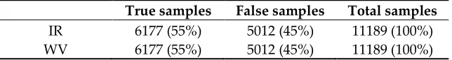
according to the SOMC dataset. Table 1 summarizes the numbers of true and false samples that both
222
make up the source dataset for our further analysis of IR and WV mosaics. The total number of
223
snapshots used (both IR and WV) is 11189. The true samples are 6177 (55%) of them, and 5012 (45%)
224
are the false samples (see Fig. 2). In order to unify images in the dataset, we normalized them by the
225
maximum and the minimum brightness temperature (in the case of IR) over the whole dataset:
226
227
= − min( )
max( ) − min( ) , (1)
228
where denotes the individual sample (represented by a matrix of 100x100 pixels), is the whole
229
dataset of 11189 IR snapshots. The same normalization was applied to WV snapshots.
230
3.2. Formulation of the problem
231
We consider MC identification as a binary classification problem. We use the set of true and false
232
samples (Figure 2) as input (“objects” herein). We have developed two DCNN architectures
233
following two conditional requirements: either (i) the object is described by the IR image only or (ii)
234
the object is described by both IR and WV images. Since the training dataset is almost target-balanced
235
(see Table 1), assuming ~50/50 ratio of true/false samples, we further use the accuracy score as the
236
measure of the classification quality. The accuracy score cannot be used as a reliable quality measure
237
of any machine learning method in the case of the unbalanced training dataset. For example, in the
238
case of a highly unbalanced dataset with the true/false ratio being 95/5 it is easy to achieve 95%
239
accuracy score by just forcing the model to produce only the true outcome. Thus, balancing the source
240
dataset with false samples is critical for building the reliable classification model.
241
242
Table 1. Total number of true and false samples.
243
True samples False samples Total samples
IR 6177 (55%) 5012 (45%) 11189 (100%)
WV 6177 (55%) 5012 (45%) 11189 (100%)
3.3. Justification of using DCNN
244
There is a set of best practices commonly used to construct DCNNs for solving classification
245
problems [55]. While building and training DCNNs for MCs identifications, we applied the technique
246
proposed by LeCun [41]. This technique implies the usage of consecutive convolutional layers which
247
detect spatial data patterns, alternating with subsampling layers which reduce the sample
248
dimensions. The set of these layers is followed by a set of so-called fully-connected (FC) layers
249
representing a neural classifier. The whole model built in this manner represents a non-linear
250
classifier capable of directly predicting a target value for the input sample. A very detailed
251
description of this model architecture can be found in [41]. We will further term the FC layers set as
252
"FC classifier," and the preceding part containing convolutional and pooling layers as "convolutional
253
core" (see Figures 3,4). The outcome of the whole model is the probability of MC presence in the input
254
sample.
255
While handling multiple concurrent and spatially aligned geophysical fields, it is important to
256
choose a suitable approach. LeCun [41] proposed the DCNN focused on the processing of only
257
grayscale images – meaning just one 2D field. In order to handle multiple 2D fields, they may be
258
stacked together to form a 3D matrix by analogy with colorful images which have three color
259
channels: red, green and blue. This approach can be applied when one uses pre-trained networks like
260
AlexNet [36], VGG16[1], ResNet [47] or similar architectures because of the original purpose of these
261
networks to classify colorful images. However, this approach should be exploited carefully when
262
applied to geophysical fields, because the mentioned networks were trained using massive datasets
(e.g., ImageNet) of real photographed scenes, which means specific dependencies laying between
264
channels (red, green and blue) within each image. In contrast to the stacking approach applied by
265
Liu et al. [39], we use separate CNN branch for each channel (IR and WV) to ensure that we are not
266
limiting the overall quality of the whole network (see Fig. 4). In the following, we describe in details
267
each DCNN architecture for both cases: IR+WV (Fig. 4) and IR alone (Fig. 3).
268
Since we consider the binary classification, and the source dataset is almost target-balanced
269
(see Tab. 1), we use as a quality measure the accuracy score or which is a rate of objects, classified
270
correctly compared to the ground truth:
271
=
1
‖ ‖
[
=
] ,
(2)where denotes the dataset and ‖ ‖ is its total samples count; is expert-defined target value
272
(ground truth), is the model decision whether the -th object contain MC.
273
In addition to the baseline which is the network proposed in [41], we applied a set of additional
274
approaches commonly used to improve the DCNN accuracy and generalization ability
275
(see Appendix A). Specifically, we used Transfer Learning (TL) [56–61] with the VGG16 [1] network
276
pre-trained on ImageNet [48] dataset; Fine Tuning (FT) [62], Dropout (Do) [63] and dataset
277
augmentation (DA) [64] (see Appendix A). With these techniques applied in various combinations,
278
we constructed six DCNN architectures that are summarized in Table 2. All of these architectures are
279
built in a common manner: the FC classifier follows the one- (for IR only) or two-branched (for
280
IR+WV) convolutional core. If the convolutional core is one-branched, its output itself is input data
281
for the corresponding FC classifier. If the convolutional core is two-branched, then concatenation
282
product of their outputs is the input data for the corresponding FC classifier. The very detailed
283
description of the constructed architectures is presented in Appendix A. For each DCNN structure
284
we trained a set of models as described in detail in section 3.5. We also applied ensemble averaging
285
(see Appendix A) of a set of models of identical configuration via averaging probabilities of true class
286
for each object of the dataset. We term these six ensemble-averaged models the “second-order”
287
models. We also applied ensemble averaging per sample of all trained DCNNs trained in this work.
288
We term this model the “third-order” model. Each of these models was trained using the method of
289
backpropagation of error (BCE loss, see Appendix A) [65] denoted as “backprop training” in Figures
290
3 and 4.
291
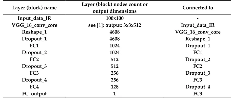
3.4. Proposed DCNN architectures
292
Six DCNNs that we have constructed are able to perform binary classification on satellite
293
mosaics data (IR alone or IR+WV) represented as grayscale 100x100px images:
294
1. 1. CNN #1. This model is built “from scratch” which means we have not used any pre-trained
295
networks. CNN #1 is built in the manner proposed in [36]. We varied sizes of convolutional
296
kernels of each convolutional layers from 3x3 to 5x5. We also varied sizes of subsampling layers’
297
receptive fields from 2x2 to 3x3. For each convolutional layers, we varied the number of
298
convolutional kernels: 8, 16, 32, 64 and 100. The network convolutional core consists of three
299
convolutional layers alternated with subsampling layers. Each pair of convolutional and
300
subsampling layers is followed by a dropout layer. CNN #1 is one-branched, and objects are
301
described by IR 500x500 km satellite snapshots only.
302
2. CNN #2. This model is built “from scratch” with two separate branches - for IR and WV data.
303
The convolutional core of each branch is built in the same manner as the convolutional core for
304
CNN #1 and as proposed in [41]. We varied the same parameters of the structure here in the
305
same ranges as for CNN #1.
306
3. CNN #3. This model is built with Transfer Learning approach. We used VGG16 pre-trained
307
convolutional core to construct this model. None of VGG16 weights were optimized within this
308
model, and only the weights of the FC classifier were trainable. This model is one-branched, and
objects are described by IR 500x500 km satellite snapshots only. CNN #3 structure is shown in
310
Fig. 3.
311
4. CNN #4. This model is two-branched, and each branch of its convolutional core is built with
312
Transfer Learning approach, in the same manner as the convolutional core of CNN #3. Input
313
data are IR and WV. None of VGG16 weights of this model in any of the two branches were
314
optimized, and only the weights of the FC classifier were trainable. CNN #4 structure is shown
315
in Fig. 4.
316
5. CNN #5 is built with both Transfer Learning and Fine Tuning approaches. We built the
317
convolutional core of this model with the use of VGG16 pre-trained network. VGG16
318
convolutional core consists of five similar blocks of layers. For the CNN #5 we turned the last of
319
these five blocks to be trainable. This model is one-branched, and objects are IR 500x500 km
320
satellite snapshots only. CNN #5 structure is shown in Fig. 3.
321
6. CNN #6 is two-branched, and branches of its convolutional core are built in the same manner as
322
the convolutional core of CNN #5. The last of five blocks of each VGG16 convolutional cores
323
were turned to be trainable. Input data are IR and WV 500x500 km satellite snapshots of dataset
324
samples. CNN #6 structure is shown in Fig. 4.
325
326
3.5. Computational experiment design
327
The following hyper-parameters are included in each of the six networks:
328
Size (number of nodes) of the first layer of FC classifier (denoted as FC1 in Figures 3,4)
329
Convolutional kernels count for each convolutional layer (only applies to CNN #1 and CNN #2)
330
Sizes of convolutional kernels (only applies to CNN #1 and CNN #2)
331
Sizes of receptive fields of subsampling layers (only applies to CNN #1 and CNN #2)
332
The whole dataset was split into training (8952 samples) and testing (2237 samples) sets stratified by
333
target value meaning that each set has the same (55:45) ratio of true/false samples as the whole dataset
334
(i.e., 4924:4028 and 1253:984 samples in training and testing sets correspondingly). We have
335
conducted hyper-parameters optimization for each of these DCNNs using stratified K-fold (K=5)
336
cross-validation approach. We trained several (typically 14-18) models with the best
337
hyper-parameters configuration on the training set for each architecture. Then we drop models with
338
the maximal and minimal accuracy score estimated with the cross-validation approach. The rest of
339
the models are evaluated on the testing set, which was never seen by the model. We estimated the
340
accuracy score for each individual model and the variance of accuracy score for the particular
341
architecture with the best hyper-parameters combination (see Table 2).
342
With the ensemble averaging approach, we evaluated the second-order models on the
343
“never-seen by the model” testing set. As described in section 3.3 we estimated the optimal
344
probability threshold for each second-order and third-order models (see Table 2) for the best
345
accuracy score estimation. These scores are treated as the quality measure of each particular
346
architecture.
347
Numerical optimization and evaluation of models were performed at the Data Center of FEB
348
RAS [66] and Deep Learning computational resources of Sea-Air Interactions Laboratory of IORAS
349
(https://sail.ocean.ru/). Exploited computational nodes contain two graphics processing units (GPU)
350
NVIDIA Tesla P100 16GB RAM. With these resources, the total GPU time of calculations is 3792
351
hours.
Figure 3. CNN #3 and CNN #5 structures. Green dots denote elements of the convolutional core
354
output reshaped to a vector, which is the fully-connected classifier input data.
355
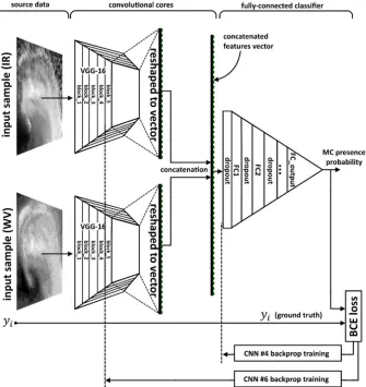
356
Figure 4. CNN #4 and CNN #6 structures. Green dots denote elements of convolutional cores outputs
357
reshaped to vectors, which are, being concatenated to a combined features vector, the fully-connected
358
classifier input data.
4. Results
360
The designed DCNNs were applied to detect of Antarctic MCs for the period from June to
361
September 2004. Summary of the results of the application of six models is presented in Table 2. As
362
we noted above, each model is characterized by the utilized data source (IR alone or IR+WV, columns
363
“IR” and “WV” in Table 2). These DCNNs are further categorized according to a chosen set of applied
364
techniques in addition to the basic approach (see Table 2 legend). Table 2 also provides accuracy
365
scores and probability thresholds estimated as described in section 3.5, for the individual, second-
366
and third-order models of each architecture.
367
368
Table 2. Accuracy score of each model with the best hyper-parameters combination. BA - basic
369
approach [41], TL - transfer learning, FT - fine tuning, Do - dropout, DA - dataset augmentation.
370
is the accuracy score averaged across models of the particular architecture. AsEA is the accuracy score
371
of the ensemble averaged models with the optimal probability threshold. is the optimal
372
probability threshold value.
373
model
name IR WV BA TL FT Do DA AsEA
CNN #1 X - X - - X X 86.89 ± 1.1 % 89.3 % 0.381
CNN #2 X X X - - X X 94.1 ± 1.4 % 96.3 % 0.272
CNN #3 X - X X - X X 95.8 ± 0.1 % 96.6 % 0.556
CNN #4 X X X X - X X 95.5 ± 0.3 % 96.3 % 0.526
CNN #5 X - X X X X X 96 ± 0.2 % 96.6 % 0.5715
CNN #6 X X X X X X X 95.7 ± 0.2 % 96.4 % 0.656
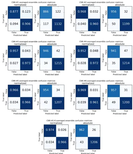
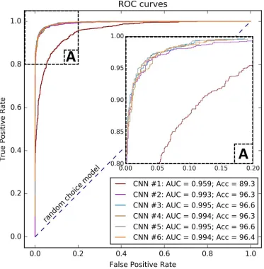
Third-order model CNN #1-6 averaged ensemble 97% 0.598
374
As shown in Table 2, CNN #3 and CNN #5 demonstrated the best accuracy among the
375
second-order models on a never-seen subset of objects. The best combination of hyper-parameters
376
for these networks is presented in Appendix B. Confusion matrices and receiver operating
377
characteristic (ROC) curves for these models are shown in Fig. 6 a-d. Confusion matrices, and ROC
378
curves for all evaluated models are presented in Appendix C. Figure 6 clearly confirms that these two
379
models perform almost equally for the true and the false samples. According to Table 2, the best
380
accuracy score is reached using different probability thresholds for each second- or third-order
381
model.
382
Comparison of CNN #1, CNN #2, on the one hand, and the remaining models, on the other hand,
383
shows that DCNNs built with the use of Transfer Learning technique demonstrate better
384
performance compared to the models built “from scratch”. Moreover, the accuracy score variances
385
of CNN #1 and CNN #2 are higher than for the other architectures. Thus, models built with Transfer
386
Learning approach seem to be more stable, and their generalization ability is better, compared to
387
models built "from-the-scratch."
388
Comparing CNN #1 and CNN #2 qualities, we may conclude that the use of an additional data
389
source (WV) results in the significant increase of the model accuracy score. Comparison of models
390
within each pair of the network configurations (CNN #3 vs. CNN #5; CNN #4 vs. CNN #6)
391
demonstrates that Fine Tuning approach does not provide significant improvement of the accuracy
392
score in case of such a small size of the dataset. It is also obvious that the averaging over the ensemble
393
members does increase the accuracy score from 0.6% for CNN #5 to 2.41% for CNN #1. However, in
394
some cases, these score increases are comparable to the corresponding accuracy standard deviations.
395
It is also clear from the last row of Table 2, that the third-order model, which averages
396
probabilities estimated by all trained models CNN #1-6, produces the accuracy of = 97% which
397
outperforms all scores of individual models and second-order ensemble models. ROC curve and
398
confusion matrices for this model are presented in Figure 6ef.
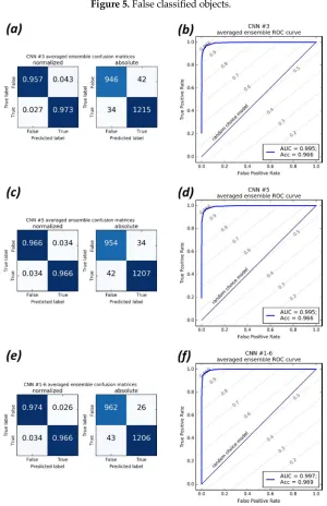
401
Figure 5. False classified objects.
402
Figure 6. Confusion matrices and receiver operating characteristic curve for (a,b) CNN #3 and (c,d)
403
CNN #5, both with the ensemble averaging approach applied (second-order models); and (e,f)
third-404
order model CNN #1-6 averaged ensemble.
Figure 5 demonstrates four main types of false classified objects. The first and the second types
406
are the ones for which IR data are missing completely or partially. The third type is the one for which
407
the source satellite data were suspected to be corrupted. These three types of classifier errors
408
originating from the lack of source data or the corruption of source data. For the fourth type, the
409
source satellite data was realistic but the classifier has made a mistake. Thus some of false
410
classifications are model mistakes, and some are associated with the labeling issue where human
411
expert could guess on the MC propagation over the area with missing or corrupted satellite data.
412
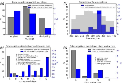
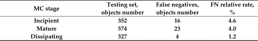
Figure 7 demonstrates the characteristics of the best model (third-order ensemble-averaging
413
model) regarding false negatives (FN). Since the testing set is unbalanced with respect to stages, types
414
of cyclogenesis and cloud vortex types, we present in Figure 7acd relative FN rates for each separate
415
class in each taxonomy. We present the testing set distribution of classes for these taxonomies as well.
416
Note that scales are different for reference distributions of classes of the testing set and the
417
distributions of missed MCs. Detailed false negatives characteristics may be found in Appendix D.
418
419
Figure 7. False negatives (missed MCs) in the never-seen by the model testing set with respect to
420
(a) lifecycle stages; (b) diameters; (c) cyclogenesis types; (d) types of cloud vortex.
421
Tracking procedure requires the sustainable ability of the MCs detection scheme to recognize
422
mesocyclone cloud shape imprints during the whole MC life cycle. Figure 7a demonstrates that the
423
best model classifies mesocyclone imprints almost equally for incipient (~4.6% incipient missed) and
424
mature (~4% mature missed) stages. The fraction of missed MCs in its dissipating stage is lower (~4%
425
missed among MCs in dissipating stage). As for distribution of missed MCs with respect to their
426
diameters (see Fig. 7b), the histogram demonstrates fractions of FN objects relative to the whole FN
427
number. The distribution of MC diameters in the testing set in Figure 7b is shown as a reference.
428
There is a peak around the diameter value of 325 km, which does not coincide with any issues of
429
distributions of MC diameters when the testing set is subset by any particular class of any taxonomy.
430
However, since the total number of missed MCs is too small, there is no obvious reason to make
431
assumptions on the origin of this issue. The FN rates per cyclogenesis types (Fig. 7c) demonstrate the
432
only issue for the orography-induced MCs. This issue is caused by the total number of that
433
cyclogenesis type, which is small (only 27 MCs in the testing set and only 134 in the training set), so
434
the 4 which were missed is a substantial fraction of it. The same issue is demonstrated for the FN
rates per cloud vortex types. Since the total number of “spiral cloud” type in the testing set is
436
relatively small (59 of 1253), the 5 missed are a substantial fraction of it, compared to 33 missed of
437
1006 for “comma cloud” type.
438
5. Conclusions and outlook
439
In this study, we present an adaptation of a DCNN method resulting in an algorithm for the
440
detection of MCs from satellite imageries of cloudiness. The DCNN technique shows very high
441
accuracy in recognition of MCs cloud signatures. The best accuracy score of 97% is reached using the
442
third-order ensemble-averaging model (6 models ensemble) and the combination of both IR and WV
443
images as input. We assess the accuracy of MCs recognition by comparison of identified MCs
444
(true/false - image contain MC/no MC on the image parameter) with a reference dataset [6]. We
445
demonstrate that deep convolutional networks are capable of effectively detecting polar mesocyclone
446
signatures in satellite imagery. We also conclude that the quality of the satellite mosaics is sufficient
447
enough for performing the task of binary classification regarding the MCs presence in 500x500km
448
patches, and for performing other similar tasks of pattern recognition type, e.g., semantic
449
segmentation of MCs.
450
Since the satellite-based studies of polar mesocyclone activity conducted in the Southern
451
Hemisphere (and in NH as well) have never reported season-dependent variations of IR imprint of
452
cloud shapes of MCs [23,27,67,68], we assume the proposed methodology to be applicable to satellite
453
imageries of polar MCs available for the whole satellite observation era in Southern Hemisphere. In
454
the Northern Hemisphere, the direct application of the models that were trained on SH dataset is
455
restricted due to the opposite sign of relative vorticity and thus, different cloud shape orientation.
456
However the proposed approach is still applicable, and the only need is a dataset of tracks of MCs
457
from the Northern Hemisphere.
458
It was also shown that the accuracy of MCs detection by DCNNs is sensitive to the single (IR
459
only) or double (IR+WV) input data usage. IR+WV combination provides significant improvement of
460
the detection of MCs and allows a weak DCNN (CNN #2) to detect MCs with higher accuracy
461
compared to the weak CNN #1 (89.3% and 96.3% correspondingly). The computational cost of DCNN
462
training and hyper-parameters optimization for deep neural networks are time- and
computational-463
consuming. However, once trained, the computational cost of the DCNN inference is low.
464
Furthermore, the trained DCNN performs much faster compared to a human expert. Another
465
advantage of the proposed method is the low computational cost of data preprocessing that allows
466
the processing of satellite imagery in real time or the processing of large amounts of collected satellite
467
data.
468
We plan to extend the usage of this set of DCNNs (Table 2) for the development of an MCs
469
tracking method based on machine learning and using satellite IR and WV mosaics. These efforts
470
would be mainly focused on the development of the optimal choice of the “cut-off” window that has
471
to be applied to the satellite mosaic. In the case of a sliding-window approach (e.g., running the
472
500x500km sliding window through the mosaics), the virtual testing dataset of the whole mosaic is
473
highly unbalanced, so a model with non-zero FPR evaluated on balanced dataset would produce
474
much higher FPR. In the future, instead of the sliding-window, the Unet-like [69] architecture should
475
be considered with the binary semantic segmentation problem formulation. Considering MC
476
tracking development, an approach proposed in a number of face recognition studies should be
477
reassuring [70,71]. This approach can be applied in a manner of triple-based training of the DCNN to
478
estimate a measure of similarity between one particular MC signatures in consecutive satellite
479
mosaics.
480
481
Author Contributions: Conceptualization, Mikhail Krinitskiy, Polina Verezemskaya and Sergey Gulev; Data
482
curation, Mikhail Krinitskiy and Matthew Lazzara; Formal analysis, Mikhail Krinitskiy; Funding acquisition,
483
Sergey Gulev; Investigation, Mikhail Krinitskiy and Kirill Grashchenkov; Methodology, Mikhail Krinitskiy and
484
Polina Verezemskaya; Project administration, Mikhail Krinitskiy; Resources, Polina Verezemskaya and Sergey
Gulev; Software, Mikhail Krinitskiy and Kirill Grashchenkov; Supervision, Sergey Gulev; Validation, Mikhail
486
Krinitskiy, Polina Verezemskaya and Sergey Gulev; Visualization, Mikhail Krinitskiy and Polina Verezemskaya;
487
Writing – original draft, Mikhail Krinitskiy, Polina Verezemskaya, Natalia Tilinina and Matthew Lazzara;
488
Writing – review & editing, Natalia Tilinina, Sergey Gulev and Matthew Lazzara.
489
Funding: This research was funded by the Russian Ministry of Education and Science (agreement 14.613.21.0083,
490
project ID RFMEFI61317X0083). Materials from MAL are based upon the work funded by the United States
491
National Science Foundation under grants ANT-1244924 and ANT-1535632.
492
Acknowledgments: Computational resources for this research were provided by the Shared Facility Center
493
“Data Center of FEB RAS”, Khabarovsk, Russia.
494
Conflicts of Interest: The authors declare no conflict of interest. The funders had no role in the design of the
495
study; in the collection, analyses, or interpretation of data; in the writing of the manuscript, and in the decision
496
to publish the results.
497
Appendix A. DCNN best practices and additional techniques
498
There is a set of best practices commonly used to construct DCNNs for solving classification
499
problems [55]. Modern DCNNs are built on the basis of consecutive convolutional and subsampling
500
layers by performing nonlinear transformation of the initial data (see Fig. 2 in [41]). The primary layer
501
type of convolutional neural networks (CNNs) is the so-called convolutional layer which is designed
502
to extract visual patterns density map using discrete convolution operation with (tends to be from
503
3 to 1000) kernels followed by a nonlinear transformation operation (activation function). One
504
additional layer type is a pooling layer performing subsampling operation with one of the following
505
aggregation functions: maximum, minimum, mean or others. In the current practice the maximum is
506
used.
507
Since the LeNet DCNN [41] several studies [41–44] have demonstrated that the usage of
508
consecutive convolutional and subsampling layers results in a skillful detection of various spatial
509
patterns from the input 2D sample. The approach proposed in [41] implies the use of the output of
510
these stacked layers set as an input data for a classifier, which in general may be any method suitable
511
for classification problems, such as linear models, logistic regression, etc. LeCun [41] suggested to
512
use the neural classifier, and this is now a conventional approach. The advantage of using a neural
513
classifier is the ability to train the whole model at once (the so-called end-to-end training).
514
The whole model built in this manner represents a classifier capable of direct predicting a target
515
value for the sample. We term the fully-connected (FC) layers set as "FC classifier", and the preceding
516
part containing convolutional and pooling layers as "convolutional core" (see Figures 3,4).
517
518
For building a DCNN it is important to account for data dimensionality during its
519
transformations from layer to layer. The input for a DCNN is an image represented by a matrix of
520
the size (ℎ, , ), where ℎ and correspond to the image height and width in pixels, is its levels
521
number, the so-called depth (e.g., = 3 when levels are red, green and blue channels of a colorful
522
image). For the water vapor or radio-brightness temperature satellite data, = 1. A convolutional
523
layer and subsampling layer are described in details in [41]. Convolutional layers are characterized
524
by their kernel sizes (e.g. 3x3, 5x5), their kernel numbers and the nonlinear operation used (e.g.
525
ℎ in [41]). Subsampling layers are characterized by their receptive field sizes e.g. 3x3, 5x5 etc. The
526
output of a convolutional layer with kernels is the so-called feature maps which is a matrix of the
527
size (ℎ, , ). The nonlinear operation transforms it to a matrix of size (ℎ, , 1). The following
528
subsampling layer reduces the matrix size depending on the subsampling layer kernel size. Typically,
529
this size is (2, 2) or (3, 3). Thus, the subsampling operation reduces the sample size by a factor 2 or 3,
530
respectively. The output of a convolutional core is a set of abstract feature maps which is represented
531
by a 3D matrix. This matrix, being reshaped into a vector, is passed as the input to the FC classifier
532
(see Figures 3,4).
533
FC classifier of all models of this study includes hidden FC layers whose count varied
534
from 2 to 4. Nodes (artificial neurons) count of FC1 which is the layer following the convolutional
535
core (see Figures 3,4), is chosen from the set {128, 256, 512, 1024}. The size of each following FC layer
is half of the preceding one, but not less than 128. The output layer is fully-connected as well and
537
contains one output node. For example, the structure of FC classifier in terms of nodes count of layers
538
might be the following: {512; 256; 128; 1}. All FC layers are alternated with dropout layers in order to
539
prevent overfitting of the model. All trainable layers’ activation functions are Rectified Linear Unit
540
(ReLU):
541
( ) = max(0; ) ,
(A1)except the output layer whose activation function is sigmoid:
542
( ) =
1
1 +
,
(A2)where are layers’ trainable parameters.
543
544
In order to measure the error of the network on each individual sample during the training
545
process we use the binary cross-entropy as a loss function:
546
ℒ =
( log
+ (1 −
)log (1 −
)) ,
(A3)where is the expert-defined ground truth for the target value, is the estimated probability of
547
the -th sample to be true, is samples count of the training set or a training mini-batch. This loss
548
function is minimized in the space of the model weights using the method of backpropagation of
549
error [65] denoted as “backprop training” in Figures 3,4. The outcome of the the whole model is the
550
probability of each class for the input sample. In the case of binary classification, the FC classifier has
551
one output unit, producing probability of MC presence for the input sample.
552
553
In addition to the basic approach proposed in [41] a number of techniques may be applied. Using
554
them one can construct and train DCNNs of various accuracy and various generalization abilities
555
which is characterized by the quality of a model estimated on a never-seen test data.
556
A.1. Transfer learning
557
One of the additional approaches is Transfer Learning [56–61]. Generally, this technique focuses
558
on storing the knowledge obtained by some network while being trained for one problem and
559
applying it to another problem of a similar kind. In practice, this approach implies the DCNN
560
structure to be built using some part of a network previously trained on a considerable amount of
561
data, for example, ImageNet [48]. In these terms, VGG16 [1] is not only an efficient architecture, but
562
also the pre-trained network containing optimized weights values (also known as network
563
parameters). Best practice for building a new advanced DCNN based on transfer learning approach
564
is to compose it using convolutional core of the pre-trained model (e.g. VGG16) followed by a new
565
FC neural classifier. Weights of the convolutional part in this case are fixed, and only FC part is
566
optimized. In this approach, the convolutional core may be considered as a feature extractor (see
567
[41]), which computes a highly relevant low-dimensional (compared to original samples
568
dimensionality) vector, representing the data (e.g. “reshaped to vector” output of the convolutional
569
core in Fig. 3).
570
A.2. Fine Tuning
571
Transfer Learning approach relies on the similarity of data distributions within two datasets.
572
But in the case of significant differences, for example in terms of Kullback–Leibler divergence
573
between some particular feature approximated probability distributions, the new FC classifier
574
capabilities may not cover all of those differences. In this case, some layers of the convolutional core,
575
that are close to FC classifier, can be turned on to be optimized (the so-called Fine Tuning). Regarding
576
DCNNs application to satellite mosaics, we have to consider that VGG16 was optimized on ImageNet
577
dataset which contains everyday-observed objects like buildings, dogs, cats, cars etc., without any
satellite imageries or even clouds. So FT approach can be considered as a promising approach when
579
composing MC-detecting DCNN at IR and WV satellite mosaic data.
580
A.3. Preventing overfitting
581
Machine learning models and neural networks in particular may vary in terms of complexity. In
582
the case of too strong model, there exist an overfitting problem: the effect of poor target prediction
583
quality on unseen data concurrently with nearly exact prediction of target values on training data.
584
There are several state-of-the-art approaches to prevent overfitting of neural networks. We used most
585
fruitful and reliable ones: dropout [63] and data augmentation also called auxiliary variables [64]. We
586
also used ensemble averaging of the models outcome.
587
A.4. Preventing overfitting with dropout
588
Dropout approach is the way of preventing overfit with a computationally inexpensive but still
589
powerful method of regularizing neural networks through bagging [72] and virtually ensembling
590
models of similar architecture. Bagging involves training multiple models and testing each of them
591
on test samples. Since training and evaluating of deep neural networks tend to be time-consuming
592
and computationally expensive, the original bagging approach [72] seems to be impractical. With the
593
dropout approach applied, the network may be thought of as an ensemble of all sub-networks that
594
can be composed by removing non-output nodes from the base network. In practice, this approach
595
is implemented by dropout layer which turns the preceding layer output to zero for each node with
596
some probability . This procedure repeats for each mini-batch at the training time. At the inference
597
time, the dropout approach involves network weights scaling by 1/ . Each of our models includes
598
dropout layers between trainable layers. Rate was set to 0.1 for each dropout layer of each model.
599
A.5. Preventing overfitting with dataset augmentation
600
Dataset augmentation is the state-of-the-art way to make a machine learning model generalize
601
better. When available dataset size is limited, the way to get around that is to generate fake data
602
which should be similar to real samples. Best practice for DCNNs is generating fake samples by
603
adding some noise or applying slight transformations like shift, shear, rotation, scaling etc. Formally,
604
with data augmentation one can increase variability of features of the original dataset and
605
substantially extend its size. This approach often improves generalization ability of the trained
606
model.
607
We trained each of our models with data augmentation approach applied. The rotation angle
608
range was 90° in both direction; independent width and height scaling performed within range from
609
0.8 to 1.2; zoom range from 0.8 to 1.2; shear angle range from -2° to 2°. We did not use flipping
610
upside-down and left-to-right.
611
A.6. Preventing overfitting with ensemble averaging
612
In general, during the parameters optimization (learning process) each DCNN converges to a
613
local minimum of the loss function in the space of its weights. The training process starts from a
614
randomly generated point of this space. Due to a non-convexity of loss function, every new DCNN
615
model converges to a new local minimum. Some models may converge to a minimum that is not
616
really close to a global one in terms of loss function value, and thus the quality measure of that model
617
remains poor. Other models may converge to a good minimum that is close to a global one in terms
618
of loss function value, but this proximity may lead to a poor generalization ability which means low
619
quality measure estimated on a testing subset of data. There are approaches for improving the
620
generalization ability of several models that are generally similar, but differ in detailed predictions.
621
In our study we applied simple ensemble averaging [73], which is one of state-of-the-art approaches
622
for improving machine learning models generalization ability. With this approach several models of
623
each architecture are trained, and probabilities of these models are averaged. The prediction of this
624
model is treated as an ensemble outcome:
=
( )
,
(A4)where is the estimated probability of the ensemble of models for -th sample to be true; each
626
-th model`s probability estimation for -th sample to be true is ( ). In this study we applied
627
ensembling on DCNNs of identical architectures. The resulting models we term second-order models
628
in this study. They are synthetic ones that are not trained, but are ensembles.
629
Satellite IR+WV snapshots or satellite IR snapshot alone are essentially the object description,
630
and each model that is presented in our study produces the outcome for each object regardless of the
631
description - whether it is IR snapshot alone or IR+WV snapshots. So there is an opportunity to
632
average probability outcomes of all the models of this study. The resulting model that produces
633
averaged probabilities of the ensemble containing all trained models we term third-order model. It is a
634
synthetic one that is not trained, but is an ensemble.
635
A.7. Adjustment of the probability threshold
636
The outcome of each model of this study is the estimation of the probability for the sample to be
637
true (i.e. to contain an MC). So there is an arbitrariness in choosing the threshold of this probability
638
to get the outcome which is binary. The most common way to choose this threshold is the ROC curve
639
analysis. Each point of this curve represents the False Positive Rate (FPR) and True Positive Rate
640
(TPR) combination for the particular probability threshold (e.g. see Fig. 6bdf). The model
641
performing true random choice between true and false outcome has a ROC curve on the main
642
diagonal of this plot. The ROC curve of the perfect classifier follows from the point (0.0, 0.0) straight
643
to the point (0.0, 1.0) and then to the point (1.0, 1.0). The area under the ROC curve (AUC ROC) may
644
be considered as a measure of model quality. The best model AUC ROC is 1.0, the true random choice
645
model AUC ROC is 0.5, and the worst model AUC ROC is 0.0.
646
In a range of cases the best accuracy score might not be reached with = 0.5. The lines of equal
647
accuracy score, as presented in Fig. 6bdf, are diagonal. In case of perfect 50/50 ratio of true/false
648
samples they are parallel to the main diagonal. In case of slight inequality of true and false samples
649
count these lines have slightly different slope as shown in Fig. 6bdf. For each accuracy score there are
650
two, one or no points of the ROC curve intersection with the accuracy isoline. So if a model is
651
represented with a ROC curve, the maximum value of its is located at the point of this curve
652
where the accuracy isoline is tangent to it. For each model of this study including second- and
third-653
order models, the optimal probability threshold was estimated based on ROC curve analysis.

![Table 2. Accuracy score of each model with the best hyper-parameters combination. BA - basic approach [41], TL - transfer learning, FT - fine tuning, Do - dropout, DA - dataset augmentation](https://thumb-us.123doks.com/thumbv2/123dok_us/7917060.1314578/10.595.81.519.273.399/accuracy-parameters-combination-approach-transfer-learning-dataset-augmentation.webp)