Optimal Solution of Transportation Problem
Based on Revised Distribution Method
Bindu Choudhary
Department of Mathematics & Statistics, Christian Eminent College, Indore, India
ABSTRACT: Transportation problem is a special type of linear programming problem. The objective of this paper is
to find an optimal solution for the transportation problem which having objective function is to be maximized using new approach Revised Distribution Method, and Vogel’s Approximation Method. This new approach Revised Distribution Method is based on allocating units to the cells in the transportation matrix starting with minimum requirement or availability to the cell with minimum cost in the transportation matrix and then try to find an optimum solution to the given transportation problem .the proposed method is easy to apply both type of balanced and unbalanced transportation problem with maximize or minimize objective function.
KEYWORDS: Transportation problem. Linear programming problem, Vogel’s Method, REDI Method,
I. INTRODUCTION
The problem of transportation or distribution arises due to shipment of goods to the destination of their requirement from various sources of the origin .The transportation model or distribution model is also a part of linear programming as it also inherits the objective of minimization of cost or maximization of profit. In the case of large scale production an industry may have production centers at various locations where from the goods are sent to the warehouses or godowns further send these goods to the distribution centers for the supply to customers. In transportation model the procedure of sending goods from one destination to another is pre- determined along with their respective cost of transportation .the transportation model mainly deals that how the cost of transportation can be minimized or the revenue of transportation can be maximized by satisfying the requirement of various destination within the known constraints of different sources of supply. The transportation model was first presented by FL Hitchcock in 1941. It was further developed by TC Koopmans (1949) and GB Dantzing (1951) towards the formulation and solution of linear programming problem. It is why the transportation model is regarded as a specific type of linear programming problem which analyse the transportation of certain homogeneous goods or services from their different sources of origins to their different destination of requirements.
II.MATHEMATICAL FORMULATION OF TRANSPORTATION PROBLEM
Suppose that there are m sources and n destination. let ai be the number of supply units available at source i ( i = 1,
2,….,m) and let bj be the number of demands units required at destination j(j= 1,2,..,n) let cij represent the unit
transportation cost for transporting the units from sources i to destination j. the objective is to determine the number of units to be transported from source i to destination j so that the total transportation cost is minimum .if xij is the
number of units shipped from source i to destination j, then the equivalent lpp model will be
Minimize (Total cost) Z =
Subject to the constraint
= bj j= 1, 2...m (demand constraints)
and xij ≥ 0 for all i and j
Existence of feasible solution a necessary and sufficient condition for a feasible solution to the transportation problem is
Total supply = Total Demand =
The representation of constraints equation i.e. supply constraints and demand constraints in the matrix form is very useful in simplification to find the optimal solution that minimize the total transportation cost (table 1)
Table 1
III.TERMINOLOGY USED IN TRANSPORTATION MODEL
Feasible Solution- Non negative valves of X ij where i = 1, 2….m and j= 1, 2…n which satisfy the constraints of
supply and demand is called feasible solution
Basic Feasible Solution- if the no of positive allocation are (m+n -1) where m = number of rows and
n = number of column.
Optimal Solution- a feasible solution is said to be optimal solution if it minimize total transportation cost
Balanced Transportation Problem - a transportation problem in which the total supply from all sources is equal to the total demand in all the destinations.
Unbalanced Transportation Problem- problem which are not balance are called unbalanced.
Matrix Terminology- in the matrix the square are called cells and form columns vertically and rows horizontally.
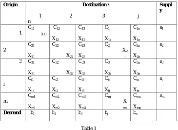
Origin Destination s
1 2 3 j n Suppl y 1 C11 X11 C12 X12 C13 X13 C1j X1j C1n X1n a1 2 C21 X21 C22 X22 C23 X23 C2j X2 j C2n X2n a2
3 C31 X31 C32 X32 C33 X33 C3j X3j C3n X3n a3 i Ci1 Xi1 Ci2 Xi2 Ci3 Xi3 Cij Xij Cin Xin ai m Cm1 Xm1 Cm2 Xm2 Cm3 Xm3 Cmj X mi Cmn Xmn am
None degenerate basic feasible solution- A basic feasible solution to a mxn transportation problem is said to be non degenerate if
1. The total number of non negative allocation is exactly m+n- 1 and
2. These m+n-1 allocation are in independent position
Degenerate Basic Feasible Solution- if the no. of allocation in basic feasible solution is less than m+n -1.
IV. A NEW APPROACH FOR SOLVING TRANSPORTATION PROBLEM
This section presents Revised Distribution Method to solve the Maximization type transportation problem which is different from the preceding method. Revised Distribution method is also easy to apply both type of balanced [1] and unbalanced transportation problem [2].
.
Step 1. Start with converting maximization problem into a minimization problem by subtracting all the elements from the highest element in the given transportation table. The modified transporting minimization problem can be solved in the usual manner.
Step 2. Start with the minimum valve in the supply column and demand row. If tie occurs, then select the demand or supply value with least cost [7].
Step 3.Compare the figure of available supply in the row and demand in the column and allocate the units equal to capacity or demand whichever is less.
Step4.If the demand in the column is satisfied, move to the next minimum value in the demand row and supply column.
Step5. Repeat steps 2 and 3 until capacity condition of all the sources demand conditions of all destination have been satisfied.
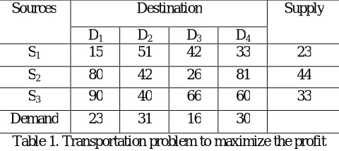
Example. the following transportation problem to maximize the profit
Sources Destination Supply
D1 D2 D3 D4
S1 15 51 42 33 23
S2 80 42 26 81 44
S3 90 40 66 60 33
Demand 23 31 16 30
Table 1. Transportation problem to maximize the profit
Sources Destination Supply
D1 D2 D3 D4
S1 75 39 48 57 23
S2 10 48 64 9 44
S3 0 50 24 30 33
Demand 23 31 16 30 100 Table 2. Transportation Matrix of the given balanced problem
In the table3 the minimum value of the demand row and supply column is 16.the cell contains smallest cost in the D3
column is 24 ie cell (S3, D3). Hence allocate the entire 16 units to this cell i.e cell (S3, D3).
Sources Destination Supply
D1 D2 D3 D4
S1 75 39 48 57 23
S2 10 48 64 9 44
S3
0 50 24
30 33
Demand 23 31 16 30 100 Table 3 First allocation of the Transportation Matrix
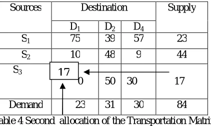
In the table 4 the minimum value of the demand row and supply column is 17.the cell contains smallest cost in the D1
column is 16 ie cell (S3, D1). Hence allocate the entire 17 units to this cell i.e cell (S3, D1).
Sources Destination Supply
D1 D2 D4
S1 75 39 57 23
S2 10 48 9 44
S3
0 50 30
17
Demand 23 31 30 84 Table 4 Second allocation of the Transportation Matrix
In the table5 the minimum value of the demand row and supply column is 6.the cell contains smallest cost in the D1
column is 10 ie cell (S2, D1). Hence allocate the entire 6 units to this cell i.e cell (S2, D1).
16
6
Table 5 Third allocation of the Transportation Matrix
In the table 6 the minimum value of the demand row and supply column is 23.the cell contains smallest cost in the S1
row is 39 ie cell (S1, D2). Hence allocate the entire 23 units to this cell i.e cell (S1, D2).
Table 6 forth allocation of the Transportation Matrix
In the table7 the minimum value of the demand row and supply column is 8.the cell contains smallest cost in the D2
column is 48 ie cell (S2, D2). Hence allocate the entire 8 units to this cell i.e cell (S2, D2).
Table 7 Fifth allocation of the Transportation Matrix
In the table 8 the remaining value of the demand row and supply column is 30.the cell contains smallest cost in the S2
row is 9 ie cell (S2, D4). Hence allocate the entire 30 units to this cell i.e cell (S2, D4).
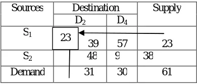
Table 8 Sixth allocation of the Transportation Matrix Sources Destination Supply
D1 D2 D4
S1 75 39 57 23
S2
10 48 9 44
Demand 6 31 30 67
Sources Destination Supply D2 D4
S1
39 57 23 S2 48 9 38
Demand 31 30 61
Sources Destination Supply D2 D4
S2
48 9 38
Demand
8 30 38
Sources Destination Supply D4
S2
9 30
Demand
30 30
6
30 23
Thus using REDI Method the basic feasible solution can be obtained as shown in table 9
Sources Destination Supply
D1 D2 D3 D4
S1
75
39
48 57 23
S2
10
48 64 9
44
S3
0 50 24
30
33 Demand 23 31 16 30 100
Table 9
Transportation cost is - 23x51 +6x80+8x42+81x30+90x17+16x66 =1173+480+336+2430+1530+1056
= 7005
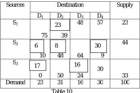
Basic Feasible solution by Vogel’s Approximation Method (Table 10)
Sources Destination Supply
D1 D2 D3 D4
S1
75
39
48 57 23
S2
10
48 64 9
44
S3
0 50 24
30
33 Demand 23 31 16 30 100 Table 10
Transportation cost is - 23x51 +6x80+8x42+81x30+90x17+16x66 =1173+480+336+2430+1530+1056
= 7005
Test for optimality
Once an initial solution is obtained the next step is to check its optimality in terms of feasibility of the solution and total minimum transportation cost .the modified distribution method is used to calculate opportunity cost associated with each unoccupied cell and then improving the current solution leading to an optimal solution .hence using the MODI Method Table 11 shown the value of ui and vj containing the cost associated with the cells for which allocation have
been made.
The opportunity cost for each of the occupied cell is determine by using the relation dij = cij - (ui + vj )
16 17
6 8 23
30
16 17
6 8 23
d11 = c11 - (u1 + v1 ) = 75- (-9+10) = 74
d13 = c13 - (u1 + v3 ) = 48-(-9+34 ) = 23
d14 = c14 - (u1 + v4 ) = 57 - (-9+9) =57
d23 = c23 - (u2 + v3 ) = 64- (0+34 ) = 30
d32 = c32 - (u3 + v2 ) = 50- (-10+48) = 12
d34=c34 - (u3 + v4 ) = 30- (-10+9 ) =31
Table 11
According to the optimality criterion for cost minimizing transportation problem the solution by REDI method is optimal. Since the opportunity costs of the unoccupied cells are zero or positive and minimum total transportation cost of Rs. 7005.
V CONCLUSION
In this paper maximize type transportation problem is solve by REDI method , and Vogel’s methods and conclude that comparatively Vogel’s method, REDI method is simple and easy to understand . This method can be used for both type of balanced and unbalanced transportation problem which is having objective function of minimize or maximize.
REFERENCES
[1] S.Aramuthakannan at el, Revised Distribution Method of finding Optimal Solution for Transportation Problems,IOSR Journal of Mathematics,
volume-4 issue-5, 2013, pp 39-42.
[2] S.Aramuthakannan at el , Application of Revised Distribution Method for Finding Optimal Solution of Unbalanced Transportation Problems, Indian Journal of Research, vol 5, issue -1, 2016, pp 32-34.
[3] Mrs. Rekha Vivek Joshi, Optimization Techniques for Transportation Problem of Three Variables,IOSR Journal of Mathematics, vol 9, issue 1,
2013, pp 46-50.
[4] Prem Kumar Gupta, D.S.Hira, Operations Research, Edition2007.
[5] J.K Sharma, Operation Research Theory and Applications, 5th Edition, 2013.
[6] Anshuman Sahu, Rudrajit Tapador, Solving the assignment problem using genetic algorithm and simulated annealing, IJAM, (2007).
[7] Hadi Basirzadeh . Ones Assignment Method for Solving Assignment Problems ,Applied Mathematical Sciences, Vol. 6, 2012, no. 47, 2345 – 2355.
Sources Destination Supply ui
D1 D2 D3 D4
S1
75
39
48 57 23 u1 = -9
S2
10
48 64 9
44 u2 = 0
S3
0 50 24
30
33
u3 = -10
Demand 23 31 16 30 100
vj v1 =10 v2 =48 v3 =34 v4 =9
23
6 8 30