Effects of Urbanization and Land-Use Changes on Low Stream Flow

UNC-WRRI-94-284

EFFECTS OF URBAN I ZATION AND LAND-USE CHANGES ON LOW STREAMFLOW

by

Jack B. E v e t t w i t h C o n t r i b u t i o n s f r o m

Margaret A. Love and James M. Gordon Department o f C i v i 1 E n g i n e e r i n g

C o l l e g e o f ~ n g i n e e r i n g

The U n i v e r s i t y o f North C a r o l i n a a t Char1 o t t e C h a r l o t t e , North C a r o l i n a 28233

The r e s e a r c h on which t h i s r e p o r t i s based was f i n a n c e d i n p a r t by t h e Department o f t h e I n t e r i o r , U.S. G e o l o g i c a l Survey, t h r o u g h t h e Water Resources Research I n s t i t u t e o f The U n i v e r s i t y o f North Carol i n a . The c o n t e n t s o f t h i s p u b l i c a t i o n do n o t n e c e s s a r i l y r e f l e c t t h e views and

p o l i c i e s o f t h e Department o f t h e I n t e r i o r , nor does mention o f t r a d e names o r commercial p r o d u c t s c o n s t i t u t e t h e i r endorsement by t h e U n i t e d S t a t e s government.

Agreement No. 14-08-0001 -G2O37 USGS P r o j e c t No. 14 (FY93)

ACKNOWLEDGEMENT

The research on which this report is based was financed in part by the United States Department of the Interior, Geological Survey, through the N.C. Water Resources Research Institute.

Margaret A. Love, a graduate student in civil engineering supported financially by the project, contributed significantly to all phases of the study. James M. Gordon, also a graduate student in civil engineering, was instrumental in developing, as part of his master's thesis, some of the statistical methodology used herein. Ms. Love contributed to the writing of the "Introduction" section; Mr. Gordon contributed to the writing of both the "Introduction" and the "Procedures" sections. Civil engineering graduate students William L. Saunders, Jr. and Scott A. Robidoux also provided assistance in conducting the project.

Specid. thanks go to Robert Mason of the Water Resources Division of the

U.S.

Geological Survey in Raleigh, NC, for providing streamflow data and helpful comments, and also to the government documents library staff of Atkins Library at The University of North Carolina at Charlotte for their generous efforts in assisting the project.

ABSTRACT

Historical low-streamflow data were analyzed for a number of gaging stations on streams in and around various urban areas in North Carolina in an attempt to find and document effects of urbanization and land-use changes on low streamflows. Records for streams within each urban area were compared with streams outside (but nearby) the urban area by two statistical methods.

It was concluded from the study that there is some support for the premise that urbanization causes a decrease in low streamflows over time, but statistically the results are inconclusive. It appears more likely that most small streams--both urban and rural--are experiencing decreasing low flows over time.

TABLE OF CONTENTS

Page

Acknowledgement

Abstract

List of Figures

List of Tables

Summary and Conclusions

Recommendations

Introduction

Purpose and Objectives

Procedures

One Sample Run Test for Randomness

Test for Equality of Slopes

Applications to Various Urban Areas

Asheville

Greensboro

Raleigh

Charlotte

Goldsboro-kin ston

Rocky Mount-Tarboro

Other Attempts

Results and Discussion

References

Glossary

Appendix A 7Q Flows (annual and five-year mean values), precipitation. and population data for stations in the Asheville area

v1

.

. .

V l l l

ix

population data for stations in the Greensboro area 85

Appendix C 7 4 mows (annual and five-year mean values), precipitation, and

population data for stations in the Raleigh area 96

Appendix D 7Q Rows (annual and five-year mean values), precipitation, and

population data for stations in the Charlotte area 105

Appendix E 7 4 Flows (annual and five-year mean values), precipitation, and

population data for stations in the Goldsboro-Kinston area 116

Appendix F 7Q Flows (annual and five-year mean values), precipitation, and

population data for stations in the Rocky Mount-Tarboro area 123

Appendix G Equality of slopes test applied to Swannanoa River at Biltmore and

LIST OF FIGURES

Page

Location Map of Stations in the Asheville Area 9

5-Year Averaged 7-Day Low Flows for Study Stations in the Asheville Area 11

Annual Precipitation for Study Stations in the Asheville Area 12

Area Population for Study Stations in the Asheville Area 13

Low-Flow Trends for Swannanoa River at Biltmore 14

Low-Flow Trends for Mills Fbver near Mills River 15

Location Map of Stations in the Greensboro Area 18

5-Year Averaged 7-Day Low Flows for Study Stations in the Greensboro Area 20

Annual Precipitation for Study Stations in the Greensboro Area 2 1

Area Population for Study Stations in the Greensboro Area 22

Low-Flow Trends for North Buffalo Creek near Greensboro 23

Low-Flow Trends for East Fork Deep River near High Point 24

Low-Flow Trends for Reedy Fork near Oak Ridge 25

Low-Flow Trends for Little Yadkin River at Dalton 26

Low-Flow Trends for Deep River at Ramseur 27

Low-Flow Trends for Hunting Creek near Harmony 28

Location Map of Stations in the Raleigh Area 30

5-Year Averaged 7-Day Low Flows for Study Stations in the Raleigh Area 32

Annual Precipitation for Study Stations in the Raleigh Area 33

Area Population for Study Stations in the Raleigh Area 34

Low-Flow Trends for Middle Creek near Clayton 35

L,ow-Flow Trends for Little Fishing Creek near White Oak 36

Low-Flow Trends for Flat River at Bahama 37

Low-Flow Trends for Deep River at Moncure

Location Map of Stations in the Charlotte Area

5-Year Averaged 7-Day Low Flows for Study Stations in the Charlotte Area

Annual Precipitation for Study Stations in the Charlotte Area

Area Population for Study Stations in the Charlotte Area

Low-Row Trends for Indian Creek near Laboratory

Low-Flow Trends for Long Creek near Bessemer City

Low-Flow Trends for Big Rear Creek near Richfield

Low-Flow Trends for Irwin Creek near Charlotte

Low-Flow Trends for McAlpine Creek at Sardis Road near Charlotte

Low-Flow Trends for Twelve Mile Creek near Waxhaw

Low-Row Trends for Long Creek near Paw Creek

Low-Flow Trends for McMullen Creek at Sharon View Road near Charlotte

Location Map of Stations in the Goldsboro-Kinston Area

5-Year Averaged 7-Day Low Flows for Study Stations

in the GoIdsboro-Kinston Area

Annual Precipitation for Study Stations in the Goldsboro-Kinston Area

Area Population for Study Stations in the Goldsboro-Kinston Area

Low-Row Trends for Nahunta Swamp near Shine

Low-Flow Trends for Contentnea Creek near Lucama

Location Map of Stations in the Rocky Mount-Tarboro Area

5-Year Averaged 7-Day Low Flows for Study Stations

in the Rocky Mount-Tarboro Area

Annual Precipitation for Study Stations in the Rocky Mount-Tarboro Area

Area Population for Study Stations in the Rocky Mount-Tarboro Area

LIST OF TABLES

Stations in the Asheville Area

Results of One Sample Run Test for Stations in the Asheville Area

Stations in the Greensboro Area

Results of One Sample Run Test for Stations in the Greensboro Area

Stations in the Raleigh Area

Results of One Sample Run Test for Stations in the Raleigh Area

Stations in the Charlotte Area

Results of One Sample Run Test for Stations in the Charlotte Area

Stations in the Goldsboro-Kinston Area

Results of One Sample Run Test for Stations in the Goldsboro-Kinston Area

Stations in the Rocky Mount-Tarboro Area

Summary of Results of the Equality of Slopes Test

Page

8

16

19 29

29

3 1 40

53

54

01

61

SUMMARY AND CONCLUSIONS

Historical low-streamflow data were analyzed for a number of gaging stations on streams in and around various urban areas in North Carolina in an attempt to find and document effects of urbanization and land-use changes on low streamflows. The urban areas included Asheville, Greensboro, Raleigh, Charlotte, Goldsboro-Kinston, and Rocky Mount-Tarboro. Records for streams within each urban area were compared with streams outside (but nearby) the urban area by two statistical methods--the One Sample Run Test and the Equality of Slopes Test. The former test checked on the randomness of data; the latter compared slopes of low-flow trends for various pairs of urban versus rural stations. The hypothesis was that low streamflows in North Carolina would exhibit a decreasing trend as urbanization progressed, with the proviso that a similar decreasing trend would not be present for nearby nonurban (rural) areas.

In the Asheville area, two rivers were considered--one urban, the other rural. Both exhibited a negative (downward) trend in low flow over time with the urban station's slope being more negative, but statistically they did not differ significantly. In the Greensboro area, two of the three urban areas had positive trends; the third was slightly negative. All of the rural stations exhibited negative trends. This outcome in itself is contrary to the project's hypothesis (that rural slopes should be greater than urban ones). The statistical analyses were, however,

inconclusive. In the Raleigh area, trends of all stations were negative, but the lone urban station did have the greatest negative slope; and the statistical analyses did tend to uphold the project's hypothesis. In the Charlotte area, trends for all stations except one--a rural one--were negative. The statistical analyses were not entirely favorable to the project's hypothesis, but the overall results did tend to uphold the hypothesis. In the Goldsboro-Kinston and Rocky Mount-Tarboro areas, the analyses were abandoned because of problems with the data.

It was concluded from the study, therefore, that there is some tendency to support the premise that urbanization causes a decrease in low streamflows over time, but statistically the results are inconclusive. It appears more likely that most small streams--both urban and rural--are

It is hoped that the results of this study will prove useful to water resource planners and regulators. The indication that low streamflows in and around urban areas appear to be decreasing with time should be helpful in future permitting actions. Additionally, proposed land-use changes within drainage basins can be considered in light of the impact the changes may have on streams which may experience decreasing low flows over time.

Further study is suggested to try to collect actual field data (as opposed to using already- collected data, as was done in this project) to develop parameters to describe the "urban" condition. Further study is also suggested to consider additional factors that might affect low streamflows. Such factors might include: time of occurrence of low flows each year;

precipitation during, or immediately preceding, the time of occurrence; maximum temperature during, or immediately preceding, the time of occurrence; stream slopes; evapotranspiration; soil sample analyses; riparian zones; and groundwater levels. It is felt in particular that the

INTRODUCTION

Most hydrological research into streamflow rates has concentrated on flood events rather than low-flow regimes. This is to be expected since uncontrolled flooding can have catastrophic consequences, which are readily apparent to the public. However, even though low-flow issues are not as visible as their high-flow counterparts, low-flow conditions play a major role in water quality and capacity problems.

Low streamflows are a matter of concern for several reasons--notably in consideration of the adequacy of a stream to supply municipal and industrial water requirements, to receive wastes (i.e., provide dispersion and dilution), to provide supplemental irrigation, and to maintain aquatic life.

It appears that much research on low streamflow has been done to quantify historical low flows rather than to identify and document specific causes of low-flow variations over time or to predict low flows (Giese and Mason 1991, Loaiciga and Marino 1988, Reynolds 1982, Riggs and Hanson 1969, Stallings 1967, Caffey et al. 1980, Vladimirov and Chebotarev 1974, Vogel and Kroll 1989). In some cases, such research has dealt with quantifying low streamflows by frequency analysis or streamflow-duration curves (Loaiciga and Marino 1988, S tallings 1967, Vladimirov and Chebotarev 1974, Vogel and Kroll 1989). Other articles deal with effects of urbanization on streamflows in general without much consideration given specifically to effects on low streamflows (Beard and Chang 1979, Hajas et al. 1978). Yet others deal with low-flow forecasting (Fish 1968, Miller and Wenzel 1985, Riggs and Hanson 1969), and others on the effects of drought on streamflow (Anderson and McCall 1968, Chang 1990, Horn 1989).

Streamflow during low-flow periods and the range of variability in low flows over time are affected by many factors but primarily are determined by a watershed's geology, climate, aild topo_praphy (Riggs 1976). These three factors all contribute to flow patterns, but one may domnate, depending on particular basin characteristics.

Soil type influences base-flow conditions by controlling infiltration and aquifer recharge. with high clay content causing more runoff (Giese and Mason 1991). Schneider (1965) has

determined that geology may be more important in determining low-flow rates than

precipitation. Streams underlain by limestone and dolomite have the greatest variability, while streams underlain by shale produce the lowest flows and streams underlain by sandstone produce the highest consistent low flows.

Many researchers have noted that urbanization contributes to decreasing low flows. For example, Leopold (1 968) reported that urbanization causes an increase in runoff and less recharge. Reynolds (1982) found a 25 percent decrease in low flows after large-scale paving of open land within a drainage basin. Fok and associates (1975) found that base flow may be reduced by as much as 30 percent by urbanization. Singh and Stall (1974) fcund that urban development caused streamflow to be reduced during low-flow periods, but not during very low flows.

smaller effect when mid-winter brings higher precipitation. Urbanization was thus found to affect both high and low flows but to be most influential in increasing the peaks of smaller floods.

On the other hand, some cases of increasing low streamflows as a result of urbanization have been reported. Spieker (1970) reported on a rapidly-urbanizing drainage area, in Salt Creek at Western Springs in Northeastern Illinois, where the 7-day, low flow exhibited a pronounced upward trend with time. Apparently the increase in impervious area, which would be expected to decrease low flow, was counteracted by other factors, such as sewer leakage and addition of wastewater effluent to the stream, both of which increase with increasing population.

Additionally, low flows may be increased substantially due to other types of development, such as golf courses which may need frequent irrigation (and provide return flow to a stream from irrigation) (Crippen 1965). Miller (1966) reported that, under extreme low-flow conditions, as much as two-thirds of the flow of Assunpink Creek in central New Jersey originates at a sewage treatment plant servicing an area that obtains its water fiom outside the basin drained by the creek.

He

also found that the return flow from 15 industrial plants along the creek totaled 2 cfs more than the 38 cfs withdrawn.

Riggs (1963), however, concluded that urbanization has little effect on low flows of streams because most drainage basins are large enough that impervious area is a small percentage of the total land area. Riggs (1965) also stated that low flows during summer and fall are better maintained in basins having a large proportion of cleared land than in those that are largely timbered. He went on to say that the influence of cleared land is greatest when the general level of discharge is lowest and that the difference becomes negligible at a high discharge level.

Several studies have looked at the impact of watershed vegetation on low flows, particularly focusing on the role of evapotranspiration in water uptake (Caffey et al. 1980, Chang and Boyer

1977, Johnson and Meginnis 1960). One of the more extensive studies was conducted at Coweeta Hydrological Laboratory in North Carolina. Swank and Douglass (1974) found that streamflow during all flow regimes was substantially reduced following plantiqg of white pines due to increased uptake of water during the growing season and increased evapotranspiration. A

similar but less dramatic effect was seen after conversion of hardwood forest to white pines, as well as following conversion of a hardwood-covered watershed to pass. Also at Coweeta, another study involved cutting trees in the riparian zone while leaving the remainder of the drainage basin forested. This produced an increase in strearnflow of 20 percent during the late summer period although less than 12 percent of the total watershed had been cut (Croft and Hoover 1951). These effects were found to be more pronounced in sunny (south-facing) slopes than in shady (north-facing) slopes at Coweeta (McNaughton and Jarvis 1983). Clearing of land in the riparian zone produces greater effects oil streamflow than clearing away from the seeam- side areas and may affect low flows even more thari higher flows (Riggs 1965). In addition, these riparian zones serve as nutrient filters between urban and agricultural areas and the stream, enhancing water quality as it travels toward the stream (Petersen et al. 1987, Hill 1990,

Lowrance et al. 1984). Johnson and Kovner (1956) found that strearnflow was increased by 4 percent due to decreased evapotranspiration after removal of only the rhododendron and laurel understory in forested areas. This finding was corroborated by Ward (1951) who found that evapotranspiration increased with vegetation height. Evapotranspiration probably has a greater efkct on the percentage of precipitation which will eventually reach the water table than any other factor, including soil conditions (LeGrand and Mundorff 1952).

areas such as the Sandhills region of North Carolina. Within residential areas of urbanized regions, lawns have been shown to have infiltration rates approximately one-sixth that of forests due to compaction (Fok et al. 1975). In areas with large clay contents, changes in land use toward increased imperviousness will not affect the infiltration rate as dramatically as changes from sandy soils to pavement (Riggs 1976). In the riparian zone, preservation of the infiltration capacity can be assured by development of greenbelts and protection of wetlands which serve as groundwater recharge areas (Singh 197 1).

The size of the drainage basin has been significantly linked to flow rates, as would be expected, with larger basins sustaining higher flows during low-flow conditions. Larger basins produce streams which are more entrenched and thus more likely to maintain a streambed below the seasonal water table, ensuring continuous-flow conditions (Singh 197 1, Singh and Stall 1974, Chiang and Johnson 1976). Larger basins will intercept more precipitation, especially during summer storms when spatial variation is greatest (Singh 197 1).

Many researchers have attempted to determine which factors have the most significant impact on streamflow during low-flow conditions. Riggs (1976) found that anything which affects

evapotranspiration rates will have the largest effect on low flows, including removal of riparian vegetation. Friel and associates (1989) found that only streamflow and size of drainage basin were statistically significantly correlated at the 95 percent level. Another study by Gebcrt (1978) showed that the most significant factors in a regression analysis where low flow was the

dependent variable were drainage area, forest cover, soil infiltration rates, and base flow. Huff and Changnon (1963) studied low streamflow in Illinois and found that precipitation data explained more than 70 percent of the low-flow variation. In the Ohio River basin, Chang and Boyer (1 977) produced statistically significant results between 7 4 10 (1 0-year recunence intenral for annual minimum of average of 7-day mean flows) values and drainage area, elevation,

percentage of forest cover, soil type, and mean annual snowfall. In southeastern Massachusetts, Tasker (1972) found that 7 4 2 (2-year recurrence interval for annual minimum of average of 7- day mean flows) and 7 4 1 0 were significantly related to drainage area and groundwater levels. However, z study in Missouri (Skelton 1974) using 7410 and drainage area in a regression analysis produced a standard error of 480 percent, while a multiple regression which included additional variables such as slope and length of basin, surface storage, annual precipitation, elevation, percentage of forest cover, rainfall intensity, and infiltration rate reduced the standard error to 250 percent. It is clear from some of these studies that one or even several factors

PURPOSE AND OBJECTIVES

The primary purpose of this project was to identify and document effects of urbanization and land-use changes on low streamflows in North Carolina, with results to be used to predict changes in low flows in areas subject to future effects of urbanization and land-use changes. Benefits would be in using the information to plan future modifications of regulations for affected areas.

The primary focus of the project was on analyzing historical low-streamflow data, with consideration given to geology, climate, and topography.

Based on information gleaned from the literature review (see preceding section), it was

PROCEDURES

The project was initiated by reviewing maps of North Carolina and selecting key U.S.

Geological Survey continuous-record, stream-gaging stations, for which low-streamflow data were available for a substantial period of time. More specifically, stations were selected from each of six "urban areasn--Asheville, Greensboro, Raleigh, Charlotte, Goldsboro-Kinston, and Rocky Mount-Tarboro. In each case, stations were identified both within and outside the

immediate urban area so that urban-rural comparisons could be made. As a general rule, at least 30 years of continuous record were required in order for a station to be included.

For each station, mean-daily flow rates for all years of record were analyzed, and " 7 4 values" were obtained for each year of record.

74

refers to the minimum average value of mean-daily streamflows for any seven consecutive days. As suggested by the American Society of Civil Engineers (ASCE), a water year from April 1 through March 31 was used in this study, the reason being to capture in a single year the entire period of late summer and early fall during which low flow is likely to occur (Loganathan et al. 1985). Annual 74 values were then plotted on a time graph for all stations in each respective urban area. Also, precipitation and population data were obtained and plotted on a time graph for each station (Figures 3, 9, 19,28,40 & 46 and 4, 10, 20, 29,41 & 47 respectively).

It was clear early on, however, that annual plotting of 7 4 values yielded a graph that was subject to significant variation from year to year, which would make visual analysis difficult. To make analyses easier but still show the low-flow trends (in other words, to "smooth" the data),

successive ten-year means of 7Q values were plotted. Thus, the mean of the ten 74 values from 1960 through 1969 was plotted, followed by the mean of the ten 7 4 values from 1961 through 1970, then fiom 1962 through 1971, and so on. The resulting plot was much "smoother" and easier to use, but it shortened the time span of available data on the plot. (For example, 30 years of record from 196 1 through 1990 provide only 21 plotted points from 1961- 1970 through 198 1 -

1990.) As something of a compromise between plotting annual values and plotting ten-year means, successive five-year means of

74

values were plotted. It was felt that this plot smoothed the data sufficiently without reducing the span of available data too much. (Thrty years of record from 196 1 through 1990 provide 26 plotted points from 196 1- 1965 through 1986- 1990.) Accordingly, all remaining plots were done using successive five-year mean values.

With plots using successive five-year mean values available for all stations in each respective urban area, a review of the stations identified for each urban area was made, resulting in the elimination of a few stations. Some were rejected because their low flows were judged to be too great to be affected by urbanization. Others were eliminated because their flows were subject to regulation, such as by a power plant dam. It was felt that such stations would not reflect

naturally-occurring low-flow conditions. On the other hand, stations with flows having diversions of water to or from them were generally not eliminated, since it was felt that such diversions were themselves quite likely manifestations of the urbanization process.

Another critical judgment was required at this point. Sicce the basis of the analysis to follow was a comparison of urban versus ma1 stations, it was essential to label each station as being either "urban" or "rural." For many stations, this designation was obvious; but for some. it was not. In fact, some stations might be in transition fiom rural to urban, but the process required that each station be classified one way or the other. Initially, it was proposed to use population data as an indicator of urban or rural, the premise being that urban areas would exhibit

others obviously rural--showed significantly-increasing population over time. Other population analyses were tried, such as using percentage increases in population rather than actual head counts and using population densities, but none proved useful. Accordingly, rural/urban

judgments were made on a station-by-station basis, considering primarily the general location of each station and the basin draining into the station.

At this point, 7 4 values and precipitation data were plotted individually for each station and a "best straight line," as determined by regression analysis, was placed on each graph to indicate trends over time. This line is referred to hereafter as the "trend line." (For two reasons--

consistency and the feeling that the most rapid urbanization has generally occurred since around 1960--these plots were made for the last 30 years or so, rather than for the entire period of record.) Stations in each urban area were then studied and analyzed to try to detect effects of urbanization on low streamflows. Two statistical methods were utilized in the analyses: the "One Sample Run Test for Randomness" and the "Test for Equality of Slopes." These nonparametric methods are described below.

ONE SAMPLE RUN TEST FOR RANDOMNESS (McCuen 1993)

Many statistical methods assume data are values of a random variable that are in sequence, but with independence between the measured values. The "One Sample Run Test" can be used to test a sample for randomness. The null hypothesis is a statement that the data represent a sample of a randomly-distributed variable. The alternative hypothesis is that one cannot conclude that the occurrence of the sample elements is not fiom an independent process. Zf the null hypothesis is rejected, the acceptance of nonrandomness does not indicate the type of nonrandomness in the sequence; but the One Sample Run Test may detect a trend or an episodic change, or ir may suggest that there is serial correlation between the measurements.

The One Sample Run Test was used to attempt to detect whether or not urban development caused a decrease in the 7-day low flow during the period of record. If a watershed undergoes urbanization during a period of record, one might expect the flow trend to decrease more than if the urbanization had not taken place. An increase in urbanization would appear as a downward trend in flow values, which represents 2 serial correlatio~? between the discharges in the annual

series of low-flow data.

The One Sample Run Test was applied to the low-flow trends (straight-line plots described previously) for

all

stations in each urban area studied to test the following null (&) and alternative (HA) hypotheses:

Ho: The 7-day low flows are randomly distributed and thus there is no signifiicant trend.

HA: There is a significant trend in the 7-day, low-flow data, since the annual data are not randomly distributed.

Critical values upon which hypothesis acceptance or rejection is based are calculated numbers that are based solely on the number of years of data that are being tested. These critical values are calculated by:

Upper value U(R) = (n

+

2)/2 (1)

Lower value L(R) = n(n

-

2)/[4(n

-

I)] ₍₂₎

where n is the number of years being tested.

The null hypothesis should be rejected if the number of runs in the sample is less than or equal to the lower critical value or greater than or equal to the upper critical value.

TEST FOR EQUALITY OF SLOPES (R. C. Tiwari, professor of statistics, UNCC, pers. com. 1992)

While the One Sample Run Test gives credibility to the hypothesis that urbanization did (or did not) result in lower streamflows for the stations studied, it was felt that additional analysis was needed to try to confirm that there was (or was not) a significant difference between the

streamflow trends for urban versus rural stations. With the assistance of Tiwari, a nonparametic method for testing equality of slopes in a simple linear model was developed and applied. The purpose of the method is to test, to a certain level of significance, two hypotheses:

Ho: The two comparative stations (urban versus rural) have the same slope (B 1 = B2).

HA: One station has a greater slope than the other one (B 1 > B2).

If the null hypothesis is accepted to a high level of significance, then the indication would be that there was little or no effect on the 7-day low flow when an area becomes urbanized. If the alternative hypothesis is accepted, then an indication of correlation between urbanization and 7- day low flow exists to an indicated level of significance.

To carry out the nonparametric model for slope comparison, a "2 value" is calculated; and a Z table is used to determine the significance level indicated by the calculated Z value. The Z value is calculated by the following formula:

N 2 0.5

Z = {T-N1[(N+1)/2] ]/{NIN~/[N(N- 1)] Z R - ~ 1 ~ 2 ( N + 1 ) 2/[4(~- I)])

1

where Z == Z -.due

T = sum of ranked numbers

N1 = number of slopes in one graph

N2 = number of slopes in other graph N = N 1 + N

When N is large, the formula used for calculating the Z value takes on a standard normal distribution, in which case the slopes are taken and analysis is made using the Central Limit Theorem. This theorem simply takes the sum of the ranked numbers, denoted by T, subtracts the expected value (E), which is represented by

and divides it by the standard deviation ( a ) indicated by

Based on computed Z values, the statistical significance of accepting the alternative hypothesis (one station has a greater slope than the other one) can be determined from a Z table.

APPLICATIONS TO VARIOUS URBAN AREAS

As indicated at the beginning of this section, stations were selected from each of six "urban areas" in North Carolina--Asheville, Greensboro, Raleigh, Charlotte, Goldsboro-Kinston, and Rocky Mount-Tarboro--for low-flow analyses. Specific details of each of these analyses follow.

Asheville

Six stations were chosen initially for study in the Asheville area. They are listed in Table 1, and their approximate locations are shown in Figure 1.

Table 1. Stations in the Asheville Area.

Drainage Area

USGS No. Statim

03439000 French Broad River at Rosman 67.9

03443000 French Broad River at Blantyre 296

0345 1500 French Broad River at Asheville 945

03453500 French Broad River at Marshall 1332

0345 1000 Swannanoa River at Biltmore 130

03436000 Mills River near Mills River 66.7

Urban/ Rural Rural Rural Urban Rural Urban Rural

The French Broad River originates in the Blue Ridge Mountains of North Carolina near the South Carolina border and flows more or less northward by stations at Rosman, Blantyre,

study as urban and Mills River, rural; and because of their close proximity, meaning similar geologic, topographic, and climatic factors, an urban versus rural comparison of low flows is appropriate.

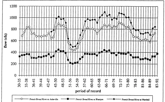
Appendix A lists the 7Q flows (annual and five-year mean values), precipitation, and population data for the Asheville-area stations, and Figures 2 through 4 exhibit the time variations for these properties. Examination of the four French Broad River stations reveals that their low-flow patterns more or less mimic each other as well as their precipitation records. The only exception is that the low-flow record for the Blantyre station appears to not decline as much as its three counterparts for the period from 1970-75 through 1985-90. This could possibly be the result of logging operations in the area. However, because of the relatively large flow rates involved (on the order of 800 cfs for the station at Asheville), it was felt that any urbanization effects on the French Broad River would be negligible at best. Hence, no further consideration was given to the four French Broad stations.

The low-flow patterns for Swannanoa and Mills Rivers (Figure 2) both exhibit downward trends for the overall period of record. Figure 5 gives a more detailed plot of flow for Swannanoa River as well as a plot of precipitation for the period of record (1962- 199 1). In each plot, a trend line is shown. The slope of the trend line for flow (-0.0178) is in units of "fractional increase (or decrease) per year." {Approximately, [(28

-

50)/50]/25 yr = -0.0 176) The slope of the trend line for precipitation (-0.2644) is in units of "inches increase (or decrease) per year." Figure 6 gives similar information for Mills River.

Inasmuch as Swannanoa River was classified as urban and Mills River as rural, it would be expected, in accord with the hypothesis stated in the "Purpose and Objectives" section, that the low-flow trend line for S wannanoa River (Figure 5) would exhibit a downward trend while the one for Mills River (Figure 6) would be more nearly "flat." Or, at least the trend line for Swannanoa River would exhibit a more downward trend than the one for Mills River. In fact, the trend line for each station is downward, with Swannanoz River (slope = -0.0178) being somewhat more downward than Mills River (slope = -0.0 126)(see Figures 5 and 6). Similarly, the precipitation trend lines are both downward, with Swannanca River (slope = -0.2644) being slightly more downward thail Mills River (slope = -0.25). While both stations exhibited

decreasing precipitation during the period, it would appear that the decline in low flow for both stations significantly exceeds that which might be attributed to decreasing precipitation alone.

The flow trend lines were first analyzed by the One Sample Run Test. Table 2 lists the annual 7 4 flows for Swannanoa River and Mills River. Median values are 35.30 cfs and 52.40 cfs, respectively. The columns in Table 2 after each

74

column include a

"+"

or 'I-" sign, depending

on whether a given 7 4 value is greater than or less than the median, respectively. The number of runs (when the data move from one side of the median value to the other) as determined from these columns is 11 for Swannanoa and 15 for Mills River. Critical values upon which

hypothesis acceptance or rejection is based were calculated using Equations (1) and (2), where n, the number of years being tested, is 29.

Figure 2 5-Year Averaged 7-Day Low Flows for Study Stations in the Asheville Area

period of record

Figure 3 Annual Precipitation for Study Stations in the Asheville Area

period of record

I

Figure 4 Area Population for Study Stations in the Asheville Area

tm

0

80,000

s

60,000

40,000

20,000

0

1960 1970 1980 ₁₉₉₀

Figure 5 Low-Flow Trends for Swannanoa River at Biltmore

#03451000

- Swannanoa River at Biltmore slope = -0.01 78

#03451000

annual precipitation, inches (5 yr avg)

Table 2. Results of One Sample Run Test for Stations in the AsheviUe Area year 62-63 63-64 64-65 65-66 66-67 67-68 68-69 69-70 70-71 71 -72 72-73 73-74 74-75 75-76 76-77 77-78 78-79 79-80 80-81 81 -82 82-83 83 -84 84-85 85-86 86-87 87-88 88-89 89-90 90-91 #0345lOOO Swannanoa 7Q 50.80 24.10 28.70 43.70 35.30 65.10 34.00 52.80 28.60 38.80 47.70 53.40 64.30 56.00 44.00 31.40 35.30 58.1 0 36.00 13.80 28.70 35.30 33.30 28.60 11.30 23.00 11.10 47.1 0 38.40 sign

+

+

+

+

+

+

+

+

+

+

+

+

+

+

+

+

Mills 7 0 47.60 32.40 60.00 52.10 54.60 101.60 63.80 104.30 41.70 66.60 46.80 55.70 72.1 0 78.10 54.30 49.80 43.00 78.30 45.30 28.70 48.80 54.40 64.1 0 46.80 28.30 52.40 27.80 113.60

40.1 0

U(R) = 15.5

Swannanoa River at Biltmore _{L(R) = 7.0}

median = 35.30

# runs = 1 1

#03446000

Mills River near Mills River

sign

+

+

+

+

+

+

+

+

+

+

+

+

+

+

median = 52.40

(It should be noted that the One Sample Run Test as well as the Equality of Slopes Test, which follows, are performed using annual low-flow data. These tests should not be contemplated with reference to Figures 5 and 6, which are plots of 5-yr average low flows.)

The flow trend lines were next analyzed by the Equality of Slopes Test. As stated previously, the first step in this test is to calculate every possible slope between two points on each graph. Then all slopes are ranked and given a rank number; and after the rank numbers are given, they (the slopes) are separated back into the watershed from which they came while still maintaining their rank numbers. These computations and rankings for Swannanoa and Mills Rivers are given in Appendix G. The first group of values in Appendix G gives the ranked slopes for Mills River, the second gives the same for Swannanoa River. The last group lists the slopes separated back into the watershed from which they came while st111 maintaining their rank number.

The expected value can now be computed by Equation (4). In this equation, N1 is 406 and N is 406

+

406, or 8 12. Hence,

The standard deviation can be calculated next using Equation (5). In this equation, N2 is 406 and

From Appendix

G,

the value of T (sum of the ranked numbers) for Mills River is 161,855.00. Hence,

With a Z value of -0.95, from a Z table, available in almost any statistics book, the statistical significaxe of accepting the alternative hypothesis (that the rural station has a greater slope than the urban one) is 65.8 percent.

Greensboro

Ten stations were chosen inj tially for study in the Greensboro area. (The Greensboro area includes Greensboro, Winston-Salem, and High Point, as well as other smaller urban locations.) They are listed in Table 3, and their approximate locations are shown in Figure 7.

Table 3. Stations in the Greensboro Area.

USGS No. Station

Drainage Area Urban/

!km

Rural

North Buffalo Creek near Greensboro Reedy Fork near Gibsonville

Deep River near Randlernan

East Fork Deep River near High Point Reedy Fork near Oak Ridge

Little Yadkin River at Dalton Haw River at Haw River

South Yadkin River near Mocksville Deep River at Ramseur

Hunting Creek near Harmony

Urban Urban Urban Urban Urban Rural Urban R u a l R u a l Rural

remaining four stations are clearly rural. Little Yadkin River at Dalton is located some 15 miles northwest of Winston-Salem and far from Greensboro; South Yadkin River near Mocksville, 25 miles southwest of Winston-Salem; Hunting Creek near Harmony, 30 miles west of Winston- Salem; and Deep River at Ramseur, 25 miles south of Greensboro.

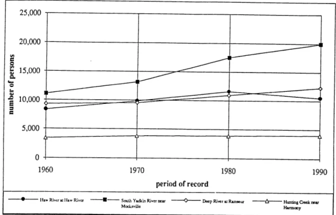
Appendix B lists the 7 4 flows (annual and five-year mean values), precipitation, and population data for the Greensboro-area stations, and Figures 8 through 10 exhibit the time variations for these properties. South Yadkin River near Mocksvllle and Haw River at Haw River were excluded at this point because of their relatively large and varying low flows and became of diversions and/or regulation. Reedy Fork near Gibsonville and Deep River near Randleman were also eliminated because of their significant regulation by several lakes upstream.

Figures 11 through 16 give more detailed plots of flow and precipitation for the remaining six stations for approximately the last 30 years. The slopes of the low-flow trend lines for the first three of these (North Buffalo Creek near Greensboro, Reedy Fork near Oak Ridge, and East Fork Deep River near High Point), all urban stations, are 0.00675,0.00498, and -0.0008, respectively. For the last three (Little Yadkin River at Dalton, Hunting Creek near H m o n y , and Deep River at Ramseur), which are rural stations, the slopes are -0.00237, -0.0024, and -0.0039. Increasing flows for two of the three urban areas may be attributable in part to increasing precipitation during the period, although two of the three rural stations showed decreasing flows despite increasing precipitation. On the face of it, however, these results, like those for the Asheville area, appear to be contrary to the overall hypothesis stated in the "Purpose and Objectives" section.

.4nalysis of these stations was performed by the One Sample Run Test, with the results shown in Table 4.

Figure 8 5-Year Averaged ?-Day Low Flows for Study Stations in the Greensboro Area

- -

period of record

Rimr nmr High -wFmkrru Oak Ridge --P-yy.L. Rim u Oritan

Figure 9 Annual Precipitation for Study Stations in the Greensboro Area

. . -

period of record

I

-Eastf%rkt)cq ~ P n k - L h * Y r a ~ ~ u

Rim na- Hi& Osk Ridge Rim .tD*lUn

1

I Point

Figure 10 Area Population for Study Stations in the Greensboro Area

period of record

I

25,000 20,000

t" 0

g

IS,OOO

a

rcl

0

V ~ u t ~ a c p

-

P x k ncu

-

in^ YM

River ncu High OetE Ridge Riw uDJtm

Poult

5,000

f h

0 I

1960 1970 1980 1990

period of record

-

I1aw Rivcr .illaw Rivcr ---- South Yadkh River

-

-

D a p R i v e r U b u

-

_{Hmhg M}

-

MocLNillc k m y

L A

1

#02095500

North Buffalo Creek near Greensboro slope = 0.00675

#02095500

annual precipitation, inches (5 yr avg)

#02093800

Reedy Fork near Oak Ridge slope = 0.00498

#02093800

annual precipitation, inches (5 yr avg)

Hunting Creek near Harmony slope = -0.0024

Figure 16 _{Low-Flow Trends for Hunting Creek near Harmony}

I

#02118500

Table 4. Results of One Sample Run Test for Stations in the Greensboro Area.

Urban/ Trend/

Rural U(R) U(L) No. Runs No Trend

North Buffalo Creek near Greensboro Urban 16.5 7.49 East Fork Deep River near High Point Urban 17.5 7.99 Reedy Fork near Oak Ridge Urban 17.5 7.99 Little Yadkin River at Dalton Rural 16.5 7.49 Deep River at Ramseur Rural 17.5 7.99 Hunting Creek near Harmony Rural 17.5 7.99

.5 no trend

S no trend .8 trend . 3 no trend .8 trend .4 no trend

Z value of 1.85, the statistical significance of accepting the altemative hypothesis (again, that the urban station has a greater slope than the rural one) is 93.6 percent. Finally, the slope of the low- flow trend line for East Fork Deep River near High Point was compared to that of Deep River at Ramseur. With a computed Z value of 3.45, the statistical significance of accepting the

altemative hypothesis (again, that the urban station has a greater slope than the rural one) is 99.9 percent.

Raleigh

Eight stations were chosen ini Raleigh, Durham, and Chapel are shown in Figure 17.

tially for study in Hill.) They are li

the Raleigh area. (The Raleigh area includes sted in Table 5, and their approximate locations

Table 5. Stations in the Raleigh Area.

USGS No. Station

Middle Creek near Clayton

Little Fishing Creek near White

Oak

Flat River at Bahama

Tar River at US 401 at Louisburg Little River near Princeton Contentnea Creek near Lucama Cape Fear River at Lillington Deep River at Moncure

Drainage Area Urban/

Rural

37.1 Urban

177 Rural

149 Rural

427 Rural

232 Rural

161 Rural

3464 Rural

1434 Rural

south and 25 miles southwest of Raleigh, respectively. Finally, Flat River at Bahama is located 25 miles northwest of Raleigh and 10 miles north of Durham.

Appendix

C

lists the

74

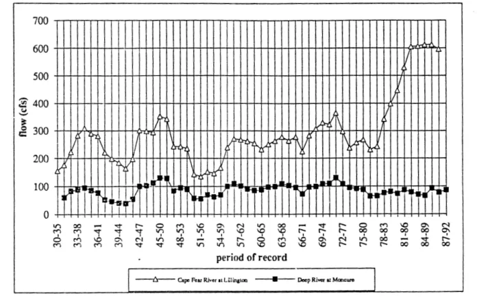
flows (annual and five-year mean values), precipitation, and population data for the Raleigh-area stations, and Figures 18 through 20 exhibit the time variations for these properties. Cape Fear River at Lillington was eliminated from further consideration at this point because of its relatively large flow and also because of its regulation--particularly by B. Everett Jordan Lake since 1981. Also excluded were Tar River at US 401 at Louisburg and Contentnea Creek near Lucama because of less than 30 years of record. The latter also experiences some regulation at low flows.

Figures 21 through 25 give more detailed plots of flow for the remaining five stations for

approximately the last 30 years. The slope of Middle Creek near Clayton, the lone urban station, is -0.0334. The slopes of the remaining four stations--Little Fishing Creek near White Oak, Flat River at Bahama, Little River near Princeton, and Deep River at Moncure--are -0.00914,

-0.0124, -0.0266, and -0.00945, respectively. While all of these slopes are negative (downward), at least the urban station has the greatest negative slope, which fact tends to support the overall hypothesis stated in the "Purpose and Objectives" section. With regard to precipitation, it appears (from Figure 21) that the decreasing low flow for the urban station greatly exceeds that which might be attributable to decreasing precipitation. For the most part, the rural stations exhibit relatively small changes in precipitation during the period.

These five stations were analyzed by both the One Sample Run Test and the Equality of Slopes Test. Results of the former are shown in Table 6.

Table 6. Results of One Sample Run Test for Stations in the Raleigh Area.

Station

Urban/ Trend/

Rural U(R)

UIL)

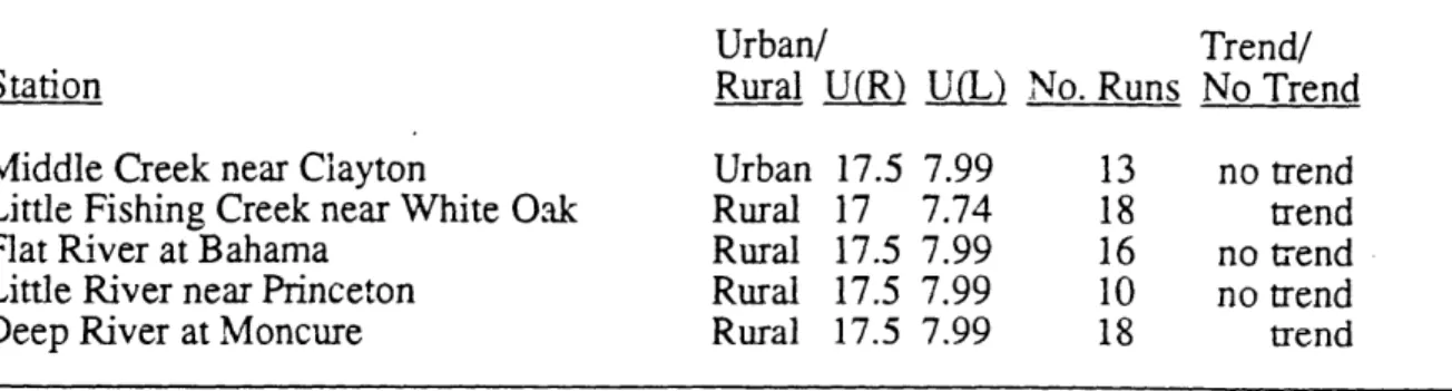
No. Runs No Trend

Middle Creek near Clayton Urban 17.5 7.99 13 notrend

Little Fishing Creek near White Oak Rural 17 7.74 18 trend

Flat River at Bahama Rural 17.5 7.99 16 notrend

Little River near Princeton Rural 17.5 7.99 10 notrend

Deep River at Moncure Rural 17.5 7.99 18 trend

The Equaiiiy of Slopes Test was applied selectively to the Raleigh-area stations. The slope of the low-flow trend line for the lane urban station--Middle Creek near Clayton--was compared separately to that of Flat River at Bahama, Little River near Princeton, and Deep River at Moncure. The Middle Creek cear Clayton-Rat River at Bahama comparison yielded a Z value of 2.21; the statistical significance of accepting the alternative hypothesis (in this case, that the

rural

station has a greater slope than the urban one) is 97.3 percent. For the Middle Creek near

Figure 19 Annual Precipitation for Study Stations in the Raleigh Area

period of record

Figure 20 Area Population for Study Stations in the Raleigh Area

16,000

14,000

12,000 r-

10,000

8,000

6,000

4,000 X

2,090

0

-

I

1960 1970 1980 1990

period of record

35,000

-

30,000

m 25,000 f

-

4

t

E

g, 20,000

csr 0

7

2

15,000

8

- --

e

E

a

=

10,000 5,000 -

0

4

I

1960 1970 1980 ₁₉₉₀

Figure 2 1 Low-Flow Trends for Middle Creek near Clayton

#02088000

Middle Creek near Clayton slope = -0.0334

#02088000

Figure 22 Low-Flow Trends for Little Fishing Creek near White Oak

#02082950

Little Fishing Creek near White Oak

slope = -0.0091 4

#02082950

Little Fishing Creek near White Oak

#02085500

Flat River at Bahama

slope = -0.01 24

#02085500

Flat River at Bahama

Figure 24 Low-Flow Trends for Little River near Princeton

#02088500

Little River near Princeton slope = -0.0266

#02088500

Charlotte

Ten stations were chosen initially for study in the Charlotte area. They are listed in Table 7, and their approximate locations are shown in Figure 26. (The two Long Creek stations are on

different streams.)

Table 7. Stations in the Charlotte Area.

USGS No. Station

Rocky River near Norwood Indian Creek near Laboratory Long Creek near Bessemer City Big Bear Creek near Richfield Zrwin Creek near Charlotte

McAlpine Creek below McMullen Creek near Pineville McAlpine Creek at Sardis Road near Charlotte

Twelve Mile Creek near Waxhaw Long Creek near Paw Creek

McMullen Creek at Sharon View Road near Charlotte

Drainage Area

(I-&

Urban/ Rur a1 Rural Rural Rural Rural Urban Urban Urban Urban Urban Urban

Unlike the Raleigh area where only one urban station could be identified, the Charlotte area has many. In fact, it was difficult to find appropriate rural statioi~s for comparison purposes. Four such rural stations identified were Rocky River near Norwood, Indian Creek near Laboratory, Long Creek near Bessemer City, and Big Bear Creek near Richfield. Rocky River near

Norwood is about 40 miles east of Charlotte; Indian Creek near Laboratory, 25 miles northwest of Charlotte; Long Creek near Bessemer City, 20 miles west of Charlotte; and Big Bear Creek near Richfield. 30 miles northeast of Charlotte. Although the Indian Creek near Laboratory station is not far south of the city of Lincolnton, it is felt that

all

these stations are properly classified as rural for this study. Long Creek near Paw Creek is located on the northwest side of Charlotte; while Irwin Creek near Charlotte, which drains the central Charlotte urban area, is on the west side. Twelve Mile Creek near Waxhaw is located some 10 miles south of the center of Charlotte, but still in a rapidly-urbanizing area. The three other stations listed in Table 7 are loczted on the south or southeast side of Charlotte; they generally drain an area that was formerly agricultural but is now urban.

Appendix

D

lists the 74 flows (annual and five-year mean values), precipitation, and population data for the Charlotte-area stations, and Figures 27 through

29

exhibit the time variations for these properties. Rocky River near Norwood was eliminated from further consideration at this point because of its relatively large flow, and McAlpine Creek below McMullen Creek near Pineville was excluded because its record goes back only 14 years.

Figure 27 5-Year Averaged 7-Day Low Flows for Study Stations in the Charlotte Area

period of record

43- wrl POD-N

Figure 29 Area Population for Study Stations in the Charlotte Area

1970 1980

period of record

I I

-

Mchfullcn Get& at

-

k i n Cruk near

-

McAlpirc Creek bclow

-

McALpk Qadt at

S h o n View Road m w Q ~ d o t t c McUullen Creek near S u d i r R o d ~

Figure 30 Low-Flow Trends for Indian Creek near Laboratory

#02143500

#02144000

Long Creek near Bessemer City slope = -0.01 81

#02 1 44000

Figure 34 Low-Flow Trends for McAlpine Creek at Sardis Road near Charlotte

#02146600

McAlpi-ne Creek at Sardis Road near Charlotte slope =

-0.00832

#02146600

#02142900

Long Creek near Paw Creek slope = -0.021 6

#02142900

annual precipitation, inches (5 yr avg)

I U O P U 1

P P P P P P

0 0 0 0 0 0

0 0 0 0 0 0

flow, cfs (5 yr avg)

P P P P P P

0 - I U O P r n

-0.01843, -0.00832, -0.02075, -0.0216, and -0.008727. With the exception of Big Bear Creek near Richfield (rural), all of these stations--rural and urban--exhibit a negative (downward) slope for the flow trend line. For the most part, all stations in this area show relatively little variation in precipitation during the period.

These stations were analyzed by both the One Sample Run Test and the Equality of Slopes Test. Results of the former are shown in Table 8.

Table 8. Results of One Sample Run Test for Stations in the Charlotte Area.

Station

Urban/ Trend/

Rural U(R) U(L) No. Runs No Trend

Indian Creek near Laboratory Rural 17.5 7.99 Long Creek near Bessemer City Rural 17 7.74 Big Bear Creek near Richfield Rural 17.5 7.99

Irwin Creek near Charlotte Urban 15.5 6.99

McAlpine Creek at Sardis Road near Charlotte Urban 15.5 6.99 Twelve Mile Creek near Waxhaw Urban 16.5 7.49

Long Creek near Paw Creek Urban 13.5 5.99

McMullen Creek at Sharon View Road near Charlotte Urban 15.5 6.99

no trend no trend trend no trend no trend no trend trend no trend

The Equality of Slopes Test was applied selectively to the Charlotte-area stations. The slope of the low-flow trend line for

rural

station Long Creek near Bessemer City, which is located 20 miles west of Charlotte, was compared separately to that of urban stations Long Creek near Paw Creek and Irwin Creek near Charlotte, both of which are on the west side of Charlotte. The Long Creek near Bessemer City-Long Creek near Paw Creek comparison yielded a Z value of 4.72; the statistical significance of accepting the alternative hypothesis (that the ma1 station has a greater slope than the urban one) is 100 percent The Long Creek near Bessemer City-Irwin Creek near Charlotte comparison yielded a Z value of 1.50, indicating a statistical significance of accepting the alternative hypothesis of 86.6 percent.

Additionally, the slope of the low-flow trend line for rural station Big Bear Creek near Richfield, which is located 30 miles northeast of Charlotte, was compared separately to those of urban stations Twelve Mile Creek near Waxhaw, McAlpine Creek at Sardis Road near Charlotte, and McMullen Creek at S h a r ~ n View Road near Charlotte,

all

of which are on the south or southeast side of Charlotte. Computed Z values of 2.34, -0.37, and -1.67 and statistical signi.fkances of accepting the alternative hypothesis of 98.1,28.9, and 90.5 percent, respectively, were

determined. In each of these cases, the alternative hypothesis is that the rural station has a greater slope than the urban one.

Goldsboro-Kinston

An attempt was made to study the Goldsboro-Kinston "urban area." Six stations were chosen for study in this area. They are listed in Table

9,

and their approximate locatioils are shown in Figure 38.

Table 9. Stations in the Goldsboro-Kinston Area.

USGS No. Station

Drainage Area Urban/

hiq

Rural

Neuse River at Smithfield 1206 Urban

Neuse River near Goldsboro 2399 Urban

Neuse River at Kinston 2692 Urban

Nahunta Swamp near Shine 80.4 Rural

Little River near Princeton 232 Rural

Contentnea Creek near Lucama 161 Rural

Kinston; while the other three would clearly be considered as rural. Nahunta Swamp near Shine is located some 12 miles northeast of Goldsboro and 20 rniles northwest of Kinston; Little River near Princeton, 10 miles east of Smithfield and 15 miles northwest of Goldsboro; and

Contentnea Creek near Lucama, 12 rniles north of Little River near Princeton.

Appendix

E

lists the

74

flows (annual and five-year mean values), precipitation, and population data for the Goldsboro-Kinston-area stations, and Figures 39 through 41 exhibit the time

variations for these properties. Because of the relatively high flows of the Neuse River (on the order of 300 to 400 cfs), it was felt that any effects of urbanization on low streamflows would be negligible; hence, the three Neuse River stations were eliminated from further consideration. This action, of course, left no possibility for urban-rural comparisons, since the remaining stations were all rural. However, because these three rural stztions' flow patterns on Figure 39 appear to show a downward trend over the last

tlurty

years or so, it was decided to consider them further.

Figures 42 and 43 give more detailed plots of flows for Nahunta Swamp near Shine and Contentnea Creek near Lucama, respectively. Corresponding plots for Little River near Princeton were given previously (Figure 24). Interestingly, all of these rural stations exhibit definite downward flow trend lines, which appear generally to decline more than might be attributed to their corresponding declines in precipitation over the same time. It is also

interesting to compare the long-term, low-flow pattern for Little River near Princeton with those for the Neuse River stations near Goldsboro and at Kinston (Figure 39). Little River near Princeton's low-flow pattern very closely mimics those for the two Neuse River stations from 1930-35 through about 1957-61. Thereafter, for an almost-equal amount of time (1957-61 through 1987-91), the Newe River stations continue with roughly the same trends

as

before, while Little River near Princeton exhibits a rather drastic decrease in low flow. It was thought that perhaps some kind of land-use change might have occurred in the Little River basin during the late 1950s that could account for the significant change in low-flow pattern. However, a spokesman for the U.S. Geological S w e y in Raleigh (Bobby Ragland, pers. corn. 1993) indicated that no such land-use change had occurred. He said this area has always been primarily agricultural. He also stated that the Survey was aware of this unusual trend, had studied it quite a bit, and had no explanation for i t

Figure 39 5-Year Averaged 7-Day Low Flows for Study Stations in the Goldsboro-Kinston

Area

period of record

-

N e ~ u Riw at SrnW=ld

-

N e w River n u GoIdsbo~o -*- Nucac R i m Y K i n s t a ~

Figure 40 Annual Precipitation for Study Stations in the Goldsboro-Kinston Area

period of record

- s- h'eusc River at S m i l l ~ c i d S Ncuse River mar Goldsboro

-

N- R i m at K i

Figure 41 Area Population for Study Stations in the Goldsboro-Kinston Area

25,000 7

20,000

V)

E:

g

I5,OOO

a

Ccl

C &

10,ooo

J

E

k

L1 i L

4 A

5,000 f s

0 I

1960 1970 1980 1990

period of record

Figure 42 Low-Flow Trends for Nahunta Swamp near Shine

#02091000

Nahunta Swamp near Shine slope =

-0.0206

#O2O9lOOO

-

Table 10. Results of One Sample Run Test for Stations in the Goldsboro-Kinston Area.

Station

Urban/ Trend/

Rural U(R) UOJ No. Runs No Trend

-

Nahunta Swamp near Shine Rural 17.5 7.99 15 no trend Little River near Princeton Rural 17.5 7.99 10 no trend Contentnea Creek near Lucama Rural 14 6.24 11 no trend

Rocky Mount-Tarboro

An attempt was also made to study the Rocky Mount-Tarboro

(Tar

River) "urban area." Six stations were chosen for study in this area. They are listed in Table 1 1, and their approximate locations are shown in Figure 44.

Table 1 1. Stations

in

the Rocky Mount-Tarboro Area.

USGS No. Station

Drainage Area

W )

02083500 Tar River at Tarboro 2183

02082506 Tar River below Tar River Reservoir near Rocky Mount 777

02082585 Tar River at NC 97 at Rocky Mount 925

02083800 Conetoe Creek near Bethel 78.1

02082950 Little Fishing Creek near White

Oak

177

02081740 Tar River at US 401 at Louisburg 427

Urban/ Rural Urban Urban Urban Rural Rural Rural

The first three Tar River stations fisted in Table 11 were characterized as urban because of their proximity to either Tarboro or Rocky Mount; the other three were judged to be

rural.

Conetoe Creek near Bethel is located approximately 10 miles southeast of Tarboro; Little Fishing Creek near White Oak, 15 miles north of Rocky Moun$ and Tar River at US 401 at Louisbarg, 30 miles northwest of Rocky Mount.

Figure 45 5-Year Averaged 7-Day Low Flows for Study Stations in the Rocky Mount-Tarboro Area

period of record

T u Kivcr at T a b

-

'Tar River k l o w Tax River Hcrrrvoir

-

Tu R i m at NC 97 SI RDcLy Mount

Figure 46 Annual Precipitation for Study Stations in the Rocky Mount-Tarboro Area

period of record

I

Figure 47 Area Population for Study Stations in the Rocky Mount-Tarboro Area

period of record

d-Tm K k c r at Tar hno Tar River bcIow Tar River Re-oir

-

Tu River at NC 97 at RoJ;). Mwnt

rcu Rocky Mount

8,000

6,000

r-l C

4,000 H

2,000 4 A

0

w _A

T

1950 1970 1980 1990

OTHER ATTEMPTS

Several other attempts to find effects of urbanization and land-use changes on low streamflows were made during the course of this study--all as yet yielding no useable results. One such attempt was to try to correlate low-flow data from a continuous-record station in a rural area with data fiom a partial-record station in a nearby urban station. Another attempt was to try to locate one or more areas of significant size that had undergone rather drastic land-use change (such as forested area to farmland or farmland to military base) within the last thirty years or so which had adequate streamflow data available to try to investigate effects of land-use change on low streamflows. No such areas were found. Yet another attempt was to study the five stations along the Yadkin River, beginning with Yadkin River at Patterson just north of Lenoir in the foothills of the Blue Ridge Mountains and continuing to Yadkin River at Yadkin College just west of High Point. The main purpose of the endeavor was to seek trends in low flows that might be attributable to land-use changes in the area. These stations were studied in the same manner as other stations previously discussed, but nothing of significance was observed. One final attempt was to plot annual 7 4 values of urban sites against concurrent

74

values of corresponding rural sites for sub-periods of record to seek significant differences in such