ANNF Estimation Technique and Methods for Finding nearest Neighbour Field

(1)

ISSN(Online): 2320-9801

ISSN (Print): 2320-9798

I

nternational

J

ournal of

I

nnovative

R

esearch in

C

omputer

and

C

ommunication

E

ngineering

(An ISO 3297: 2007 Certified Organization)

Vol. 4, Issue 9, September 2016

ANNF Estimation Technique and Methods for

Finding nearest Neighbour Field

Surase Sapna Ramhari

Student, Dept. of CSE, Maharashtra Institute of Technology, Aurangabad, Maharashtra, India

ABSTRACT: FeatureMatch, a generalised approximate nearest-neighbour field (ANNF) computation framework,

between a source and target image. The proposed algorithm can estimate ANNF maps between any image pairs, not necessarily related. To compute ANNF maps, Image patches from the pair of images are approximated using low-dimensional features, which are used along with KD-tree to estimate the ANNF map. This ANNF map is further improved based on image coherency and spatial transforms. The proposed generalisation enables us to handle a wider range of vision applications, which have not been tackled using the ANNF framework. Computing the dense Approximate Nearest-Neighbour Field (ANNF) between a pair of images has become a major problem which is being tackled by the image processing community in the recent years. Two important papers viz. Patch Match and CSH have been developed over the past few years based on the coherency between images, but one major problem both these papers have is that image patches are treated as high dimensional vector features. In this paper we present a novel idea to reduce the dimensions of a p-by-p patch of color image to a set of low level features. This reduced dimension feature vector is used to compute the ANNF. Using these features we show that instead of dealing with image patches as p2 dimensional vectors, dealing with them in a lower dimension gives a much better approximation for the nearest-neighbour field as compared to the state of the art. We further present a modification which improves the ANNF to give more accurate color information and show that using our improved algorithm we do not need a pair of related images to compute the ANNF like in other algorithms, i.e. we can generate the ANNF for all the images using unrelated image pairs or even from a universal source image.

KEYWORDS: Approximate nearest neighbour field, patch based image synthesis, PatchMatch, FeatureMatch.

I. INTRODUCTION

(2)

ISSN(Online): 2320-9801

ISSN (Print): 2320-9798

I

nternational

J

ournal of

I

nnovative

R

esearch in

C

omputer

and

C

ommunication

E

ngineering

number of patches in an image is in the millions and one needs to find Approximate Nearest Neighbors (ANN) for each patch in real or near real time. In the past, it was customary to compute ANNF with traditional approximate nearest neighbor tools such as Locality Sensitive Hashing (LSH) or KD-trees. These tools perform well in terms of accuracy but are not as fast as one would hope. Recently, a novel method, termed PatchMatch, proved to outperform those methods by up to two orders of magnitude, making applications that rely on ANNF run at interactive rate. The key to this speedup is that PatchMatch relies on the fact that images are generally coherent. That is, if we find a pair of similar patches, in two images, then their neighbors in the image plane are also likely to be similar. PatchMatch uses a random search to seed the patch matches and iterates for a small number of times to propagate good matches. Unfortunately, Patch- Match is not as accurate as LSH or KD-trees and increasing its accuracy requires more iteration that cost much more time. In addition, the main assumption it relies on (i.e. coherency of the image) becomes invalid in some cases (e.g. in strongly textured regions), with noticeable influence on mapping quality. It is therefore beneficial to develop an algorithm that is as fast, or faster, than PatchMatch, and more accurate. Approximate Nearest Neighbour Field (ANNF) computations are a recent development in the image processing communities which have gained wide popularity, especially in the graphics community, due to their fast computation times. Though being widely used by the graphics community, ANNF computations have not been widely adapted for solving other image processing problems. One of the main reasons for this is that for ANNF computations, related pair of images are conventionally used, and in cases where such related pair of images are not available, different regions from a single image are used. In this paper, we generalize the ANNF technique beyond related image pairs. This generalization expands the scope of the ANNF computation to various image processing applications. The problem of finding nearest neighbour field (NNF) in images, as illustrated in Fig. 1, is defined as: “Given a pair of images (target and source), for every p× p patch in the target image, find the closest patch in the source image (minimum Euclidean distance, or any other appropriate measure).” This mapping, from every p × p patch in target image to source image is called the NNF mapping. This mapping between a pair of images or between an image and a set of images has been crucial in a number of applications. The complexity, even for a relatively small image size, say 800×600 pixels, where each image has nearly half a million p× p patches, results in O(N2) ≈ 200 billion computations, if done using brute force. For NNF mapping, many of the existing exact nearest neighbour algorithms like (Bentley, 1975) and (Sproull, 1991) can be used, by treating each p-by-p patch as a point in p2 - dimensional Euclidean space. The drawback in this solution is based on the observation that a p-by-p image patch is not just a p2 dimensional point, it has various spatial features like edges, corners, textures etc. Also there exists a spatial relation between adjacent patches in an image which is completely disregarded in this solution. (Neeraj Kumar, 2008) solved the NNF problem by taking the inherent image properties into consideration, and showed that vp-trees provide the best result in computing the nearest-neighbours.

Fig.1: Similar patches in the pair of images

(3)

ISSN(Online): 2320-9801

ISSN (Print): 2320-9798

I

nternational

J

ournal of

I

nnovative

R

esearch in

C

omputer

and

C

ommunication

E

ngineering

neighbour. KD-tree search introduced by (Sunil Arya, 1998) is one such ANN method, which works in O (kd × log n)

time (k-nearest neighbours are found from n vectors of d-dimensions each). Another approach is based on hash tables which exploit the property that points which are close together have a higher probability of colliding. Locality Sensitive Hashing (LSH) (Piotr Indyk, 1998)works on this basis for d-dimensional points. Both these methods were developed for d-dimensional vectors, and do not take into consideration any image properties. Color image patches can be approximated to low dimensional feature vectors and then conventional k-nearest neighbor algorithms can be used effectively on these feature vectors. Conventional k-nearest neighbor algorithms do not take into consideration any of the image properties. Due to this, we incorporate image coherency, as used by Patch Match and CSH, into our proposed approach to improve upon the ANNF mapping obtained using the reduced dimension features. Apart from computing ANNF more efficiently, we expand the ANNF computation beyond related pairs of colour images to more general cases. Before venturing into the general cases of ANNF mappings, we describe the conventional methods in which ANNF mappings are used.

II. MOTIVATION

Nowadays the problem of finding the nearest neighbors is of major importance to a variety of applications. Mostly for similarity searching we can use the technique of finding nearest neighbors in many applications such as for information retrieval, object detection, pattern recognition etc. The ANNF computations are used widely for finding the nearest neighbor in many image processing applications which have gained wide popularity, especially in the graphics community due to their fast computation times. In the context of image processing Approximate Nearest Neighbour Field computations are used widely by the graphics and computer vision community to deal with problems like image completion, retargeting, denoising, optic disk detection etc. due to their fast computation times.

III. NECESSITY

Nowadays finding the similar patches is very important task in many areas. We require searching of a set of images for similar patches which is very expensive operation. The need to quickly find the nearest neighbor to a query point arises in a variety of geometric applications. The nearest neighbor’s problem is of major importance to a variety of applications: Like data compression, databases and data mining, information retrieval, machine learning, pattern recognition etc.

IV. Objective :

To generalize the ANNF technique beyond the related image pairs, because for ANNF computations, related pair of images are conventionally used and in cases where such related pair of images are not available, different regions from a single image are used. This generalization helps to expand the scope of ANNF computation to various image processing applications. To compute ANNF maps ANNF computations are used, these ANNF maps are used widely by the graphics and computer vision community to deal with problems like image completion, image retargeting, image denoising, optic disk detection, etc.

V. APPROXIMATE NEAREST NEIGHBOR FIELDS

The aim of Nearest Neighbour Field computation between a pair of images, say target (T) and source (S) can be defined as:

“For every p× p patch (t) in the target image, find the closest patch (st) in the source image by minimising the distance (d) between t and st. The metric d can be Euclidean or any other appropriate measure.” The NNF map F over every p × p patch in target image T is defined as:

F (xt) = θt

s.t. θt= arg min ( θ(S), t) (1)

F maps a target patch ‘t’ at location ‘xt’ to a transformation vector θt, where θt∈ RNconsists of parameters

(4)

ISSN(Online): 2320-9801

ISSN (Print): 2320-9798

I

nternational

J

ournal of

I

nnovative

R

esearch in

C

omputer

and

C

ommunication

E

ngineering

• Atcaptures the location, size, rotation, scale and other spatial transformations. • βtcaptures the colour, intensity and other range transformations.

Using the NNF map, we obtain the reconstructed target image ( ), as the union of source image patches. The source image patches are obtained from the block transformations for each target image patch, i.e.:

( ) = ⋃ θt (S) =⋃ st (2)

As can be observed from the formulation of NNF problem, there is no inherent restriction on what can constitute a source image and target image. Existing approaches like PatchMatch, CSH etc. have approximated the NNF computation to a pair of related images, since computing the transformations θtunder all possible spatial and range transforms become computationally intractable. Hence while computing the ANNF map, existing approaches adapt various strategies to approximate the transformation θt.

VI. FEATURE MATCHING

(5)

ISSN(Online): 2320-9801

ISSN (Print): 2320-9798

I

nternational

J

ournal of

I

nnovative

R

esearch in

C

omputer

and

C

ommunication

E

ngineering

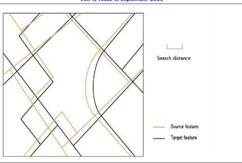
Fig. 2: Illustration of similar but inconsistent datasets for feature matching

For example, if one source feature spatially matches two candidate target features, but one of the target features has matching attribute values and the other doesn't, then the former is chosen as the final match. The condition of attribute match affects the level of confidence of the feature matching.

VII. METHODS FOR FINDING NEAREST NEIGHBORS

We now describe various methods for finding nearest neighbors. To give a moreintuitive idea of how the different methods operate, a simple 2D dataset partitioned using each of the methods is shown in Fig. 3.

Fig. 3: The partitioning of a 2D point set using different types of nearest neighbor trees

kd-trees

(6)

ISSN(Online): 2320-9801

ISSN (Print): 2320-9798

I

nternational

J

ournal of

I

nnovative

R

esearch in

C

omputer

and

C

ommunication

E

ngineering

the split value. Choosing the dimension with maximum variance leads to smaller trees, while the split value is usually chosen to be the median value along the split dimension. This results in a balanced partitioning of points into axis-aligned hyper-rectangles, which get smaller in regions with many points as in Fig. 3(a). The kd-tree exhibits many favorable properties and has proven to be quite efficient in practice for low-dimensional data. However, it has a few drawbacks:

1. The number of neighbors for each leaf node grows exponentially with dimension, causing search to quickly devolve into a linear scan.

2. The node divisions are always axis-aligned, regardless of the data distribution. This often results in poor search performance.

In real applications, the first problem is typically skirted by relaxing the requirement that all close neighbors be found. The Best Bin First (BBF) (Lowe, 1997) approach is one such technique. It is based on the observation that the vast majority of the neighboring cells usually do not contain a nearest neighbor. It therefore searches the candidate cells in ascending order of their distance to the query, and terminates the search early to save computations. It is claimed that this method produces 95% of the correct neighbors at 1% the cost of an exhaustive search for one particular application.

PCA trees

(Sproull, 1991) Attempts to remedy the axis-alignment limitation of kd-trees by applying Principal Components Analysis at each node to obtain the eigen-vector corresponding to the maximum variance and splits the points along that direction. This is equivalent to rotating the points about their mean such that their maximum variance now lies along the primary axis. We have implemented this variant as well, calling it the PCA Tree. For an example of what a tree partitioned using this method looks like, see Fig. 3(b).

Ball trees

The kd-tree and its variants can be termed “projective trees,” meaning that they categorize points based on their projection into some lower-dimensional space. In contrast, all our remaining methods are “metric trees” – structures that organize points based on some metric defined on pairs of points. Thus, they don’t require points to be finite-dimensional or even in a vector space. The first type of metric tree that we will look at is ball trees (Ommohundro, 1989). In their original form, each node’s points are assigned to the closest center of the node’s two children. The children are chosen to have maximum distance between them, typically using the following construction at each level of the tree. First, the centroid of the points is located, and the point with the greatest distance from this centroid is chosen as the center of the first child. Then, the second child’s center is chosen to be the point farthest from the first one. The resulting division of points can be understood as finding the hyperplane that bisects the line connecting the two centers, and perpendicular to it as in Fig. 3(c). Note that in this construction, there is no constraint on the number of points assigned to either node and the resulting trees can be highly unbalanced. While unbalanced trees are larger (and take longer to construct) than their balanced counterparts, this does not mean that they will be slower to search. On the contrary, such trees might be significantly faster if they capture the true distribution of points in their native space.

k-Means

(7)

ISSN(Online): 2320-9801

ISSN (Print): 2320-9798

I

nternational

J

ournal of

I

nnovative

R

esearch in

C

omputer

and

C

ommunication

E

ngineering

Vantage Point Trees

We turn now to a metric tree that uses a single “ball” at each level the vantage point tree (vp-tree). Rather than partitioning points on the basis of relative distance from multiple centers (as was the case with ball trees and k-means), the vp-tree splits points using the absolute distance from a single center. This approach can be visualized as partitioning points into “hypershells” of increasing radius, e.g., Fig. 3(d). The center of each node can be chosen randomly, as the centroid of the points, or as a point on the periphery (to maximize the distance between points). The number and thickness of the “hypershells” can also be chosen in various ways.

VIII. CONCLUSION

Approximate nearest neighbour field computations are widely used. Feature match is a generalised Approximate nearest neighbour field computation framework, between a source and target image. In this work, we have extensively evaluated a number of different approaches for solving the nearest neighbors problem. In particular, we have focused on using these approaches for finding similar image patches. Since this is a common step in a wide range of applications ranging from object recognition and texture synthesis to image denoising and compression, solving this problem efficiently will lead to faster solutions for all of these disparate tasks.

REFERENCES

[1]. S. Arya, D. M. Mount, N. S. Netanyahu, R. Silverman, and A. Y. Wu, ‘An optimal algorithm for approximate nearest neighbor searching fixed dimensions,’ J. Amer. Comput. Mater., vol. 45, no. 6, pp. 891–923, 1998.

[2]. J. L. Bentley, ‘Multidimensional binary search trees used for associative searching,’ Commun. ACM, vol. 18, no. 9, pp. 509–517, 1975. [3]. R. F. Sproull, ‘Refinements to nearest-neighbor searching in k-dimensional trees,’ Algorithmica, vol. 6, no. 4, pp. 579–589, 1991.

[4]. N. Kumar, L. Zhang, and S. K. Nayar, ‘What is a good nearest neighbors algorithm for finding similar patches in images?’ in Proc. ECCV, 2008, pp. 364–378.

[5]. P. Indyk and R. Motwani, “Approximate nearest neighbors: Towards removing the curse of dimensionality,” in Proc. ACM Symp. Theory Comput., 1998, pp. 604–613.

[6]. Beis, J.S., Lowe, D.G.: Shape indexing using approximate nearest-neighbour search in high-dimensional spaces. CVPR (1997). [7]. Omohundro, S.M.: Five balltree construction algorithms. Technical Report 89-063 (1989).

[8]. MacQueen, J.: Some methods for classification and analysis of multivariate observations. Symposium on Mathematical Statistics and Probability (1967) 281–297.

[9]. Bentley, J.L.: K-d trees for semidynamic point sets. Symposium on Computational geometry (1990) 187–197.

[10].Hays, J., Efros, A.A.: Scene completion using millions of photographs. ACM Transactions on Graphics (SIGGRAPH) 26(3) (2007). [11].Edelsbrunner, H.: Algorithms in combinatorial geometry. Springer-Verlag, New York, NY (1987).