Fiber Length Measurement by Image Processing

ABSTRACT

IKIZ, YUKSEL. Fiber Length Measurement by Image Processing. (Under the direction of Dr. Jon P. Rust.)

This research studied the accuracy and feasibility of cotton fiber length measurement by image processing as an alternative to existing systems. Current systems have some weaknesses especially in Short Fiber Content (SFC) determination, which is becoming an important length parameter in industry.

Seventy-two treatments of five factors were analyzed for length and time measurements by our own computer program. The factors are: Sample preparation (without fiber crossover and with fiber crossover), lighting (backlighting and frontlighting), resolution (37-micron, 57-micron, 106-micron, and 185-micron), preprocessing (4-neighborhood and 8-neighborhood), and processing (outlining, thinning, and adding broken skeletons).

The best results in terms of accuracy, precision and analysis time for images without fiber crossovers were: 106-micron resolution with frontlighting using an 8-neighborhood thresholding algorithm and using an outline algorithm for length determination. With fiber crossovers, 57-micron resolution with backlighting using an 8-neighborhood thresholding algorithm and using a thinning algorithm combined with an adding algorithm for combining broken skeletons. Using the above conditions, 1775

2

Fiber Length Measurement

by Image Processing

by

Yuksel Ikiz

A dissertation submitted to the Graduate Faculty of North Carolina State University

in partial fulfillment of the requirements for the Degree of

Doctor of Philosophy

FIBER AND POLYMER SCIENCE

Raleigh 2000

APPROVED BY:

_________________________

_________________________

_________________________

_____

____________________

DEDICATION

BIOGRAPHY

ACKNOWLEDGMENTS

I wish to express my deep appreciation to Dr. Rust, my major advisor, for his encouragement, guidance, and support throughout every phase of this research. Whenever I had a problem, his help was right there for me as an advisor and as a friend. I want to give special thanks to Dr. Trussell, my minor representative, for his valuable advice and determination. He read each sentence carefully and questioned each fuzzy point, which resulted in a better final product.

My sincere thanks to Dr. Barnhardt, former Dean of College of Textiles, for his genuine interest and advice. I am grateful to Dr. Jasper for his help, support and discussions. I also thank Dr. Pourdeyhimi for his advice and the use of his equipment.

TABLE OF CONTENTS

LIST OF TABLES...vii

LIST OF FIGURES...ix

1. INTRODUCTION...1

2. LITERATURE REVIEW...4

2.1. INTRODUCTION OF LENGTH...4

2.1.1. Variability...4

2.1.2. Length Distribution...8

2.1.3. Definitions...15

2.1.3.1. Staple Length (STPL)...16

2.1.3.2. Mean Length (ML)...17

2.1.3.3. Upper-Quartile Length (UQL)...18

2.1.3.4. Effective Length...18

2.1.3.5. Modal Length...19

2.1.3.6. Span Length (SL)...19

2.1.3.7. Upper-Half-Mean Length (UHML)...20

2.1.3.8. Uniformity Index (UI)...20

2.1.3.9. Uniformity Ration (UR)...21

2.1.3.10. Short Fiber Content (SFC)...21

2.1.3.11. Floating Fiber Index (FFI)...22

2.1.4. Cross Examinations of Different Lengths...22

2.2. MEASUREMENT SYSTEMS...24

2.2.1. Array Method...25

2.2.2. Fibrograph...28

2.2.3. HVI-Spinlab...30

2.2.4. HVI-MCI...31

2.2.5. Peyer Almeter AL-101...32

2.2.6. AFIS...34

2.2.7. Conclusion...39

2.3. IMPORTANCE OF LENGTH...41

2.3.1. Length Related to Other Fiber Properties...42

2.3.2. Length Related to Spinning Process and Yarn Quality...43

2.4. SHORT FIBER CONTENT...45

2.5. IMAGE PROCESSING IN LENGTH MEASUREMENT...48

2.5.1. Lighting...49

2.5.2. Image Acquisition...50

2.5.3. Image Processing...53

3. RESEARCH APPROACH...60

3.1. OBJECTIVE...60

3.2. APPROACH...60

4. EXPERIMENTAL...63

4.1. SAMPLE PREPARATION...65

4.2. LIGHTING...67

4.3. RESOLUTION...70

4.5. PROCESSING...73

4.5.1. Outline...74

4.5.2. Thinning...75

4.5.3. Erosion and Dilation...76

4.5.4. Crossover...77

4.6. STATISTICAL ANALYSIS...78

5. PRERESULTS AND PREDISCUSSION...79

5.1. IMAGE CONSTRUCTION...79

5.2. MASKING...81

5.3. THRESHOLD SELECTION...81

5.4. FIBER ORIENTATION...84

5.5. IMAGE PROCESSING VARIATION SOURCES...85

6. RESULTS AND DISCUSSION...87

6.1. HAND-MEASUREMENT...87

6.2. IMAGE PROCESSING...88

6.2.1. Without Fiber Crossover-37 micron Resolution-Backlighting...88

6.2.2. Without Fiber Crossover-37 micron Resolution-Frontlighting...96

6.2.3. Without Fiber Crossover-57 micron Resolution-Backlighting...102

6.2.4. Without Fiber Crossover-57 micron Resolution-Frontlighting...108

6.2.5. Without Fiber Crossover-106 micron Resolution-Frontlighting...113

6.2.6. Without Fiber Crossover-185 micron Resolution-Frontlighting...119

6.2.7. With Fiber Crossover-37 micron Resolution-Backlighting...124

6.2.8. With Fiber Crossover-57 micron Resolution-Backlighting...129

6.2.9. With Fiber Crossover-57 micron Resolution-Frontlighting...134

6.3. HVI AND AFIS...138

6.4. SUMMARY………..139

7. CONCLUSION...146

8. RECOMMENDATIONS FOR FURTHER RESEARCH ………150

9. REFERENCES...152

LIST OF TABLES

Table 2.1: Cotton variability classification………..4

Table 2.2: Percentage errors of normal distribution………5

Table 2.3: Percentages of length variances from full data set attributable to between lab, instrument and sample variability………7

Table 2.4: Percentages of uniformity variances from full data set attributable to between lab, instrument and sample variability……….7

Table 2.5: USDA standard deviation requirements……….8

Table 2.6: Cotton classification according to staple length………...17

Table 2.7: Cotton classification according to UQL………...18

Table 2.8: U.S. Upland cotton uniformity index………...21

Table 2.9: U.S. Upland cotton uniformity ratio……….21

Table 2.10: Some correlation coefficients between different length measurements…….23

Table 2.11: Fiber length array method………..26

Table 2.12: ASTM interlaboratory test results………..27

Table 2.13: ASTM 95% confidence interval significant levels……….28

Table 2.14: Components of variance of Fibrograph calculated from test results and expressed as standard deviations………...29

Table 2.15: Critical differences between two means in cotton fiber length tests………..29

Table 2.16: Components of variance and critical differences of HVI-Spinlab…………..31

Table 2.17: Components of variance and critical differences of HVI-MCI………..32

Table 2.18: Peyer length measurement comparison………..34

Table 2.19: Variance components of Peyer………...34

Table 2.20: AFIS length accuracy test………...37

Table 2.21: AFIS measurement variability on SFC and UQL………...37

Table 2.22: Some correlation coefficients of AFIS versus Suter-Webb………38

Table 2.23: Staple length expected and measured values………..38

Table 2.24: UQL, ML, and SFC comparisons of length measurement systems…………39

Table 2.25: Correlation coefficients between measurement systems………40

Table 2.26: Correlation coefficients between measurement systems………40

Table 2.27: Measurement methods of the existing systems………..40

Table 2.28: Production and value of cotton in US……….41

Table 2.29: Span length effect on the cotton prices………...41

Table 2.30: Parameters affected by fiber length………43

Table 2.31: Relative contribution of fiber properties to yarn SBF of ring spun…………45

Table 2.32: Relative contribution of fiber properties to yarn SBF of open-end…………45

Table 2.33: Parameters affected by SFC and UI………46

Table 2.34: Low-pass filter convolution masks……….54

Table 2.35: High-pass filter convolution masks………54

Table 4.1: Experimental design……….66

Table 6.1: 30 individual polyester fiber hand-measurement results………..88

Table 6.2: Length measurement results of images without crossover-backlighting-37 micron resolution (10xmm)………...92

LIST OF FIGURES

Figure 2.1: Length reproducibility (+/- 0.02 inches)………...7

Figure 2.2: Uniformity reproducibility (+/-1.0 %)………..7

Figure 2.3: Staple diagram………...8

Figure 2.4: Weight-length and number-length distributions………...9

Figure 2.5: Random caught fibers and fibrogram curve………11

Figure 2.6: Fibrogram of fibers as caught in a draft zone……….12

Figure 2.7: Frequency diagram, staple diagram, fibrogram, and beard diagram………...15

Figure 2.8: Effective length………...19

Figure 2.9: AFIS fiber individualizer……….35

Figure 2.10: Electro-optical sensor………36

Figure 2.11: Diffuse frontlighting technique……….49

Figure 2.12: Collimated backlighting………50

Figure 2.13: Backlighting with condenser lens………..50

Figure 2.14: CCD operation………..52

Figure 2.15: Image of three cotton fibers with 4 gray levels……….55

Figure 2.16: Image of three cotton fibers with 256 gray levels……….56

Figure 2.17: Application of different thinning algorithms………57

Figure 2.18: Image of 4 gray level polyester fibers with frontlighting technique……….59

Figure 4.1: Backlighting………68

Figure 4.2: Directional frontlighting………..69

Figure 4.3: 226x884, 37-micron, backlighting………..71

Figure 4.4: 223x508, 57-micron, frontlighting………..71

Figure 4.5: 223x189, 106-micron, frontlighting………72

Figure 4.6: 238x133, 185-micron, frontlighting………72

Figure 4.7: 4 neighborhood………72

Figure 4.8: 8 neighborhood………72

Figure 4.9: Chain code of neighbor pixels………74

Figure 4.10: Outline applied image………...75

Figure 4.11: Thinning applied image...………...76

Figure 4.12: Dilation applied image………..77

Figure 5.1: Original image from camera………80

Figure 5.2: Constructed image………...80

Figure 5.3: Low-pass filter applied………81

Figure 5.4: High-pass filter applied………...81

Figure 5.5: 4-neighborhood, threshold 6………82

Figure 5.6: 8-neighborhood, threshold 6………82

Figure 5.7: 4-neighborhood, threshold 8………82

Figure 5.8: 8-neighborhood, threshold 8………82

Figure 5.9: 4-neighborhood, threshold 20………..83

Figure 5.10: 8-neighborhood, threshold 20………83

Figure 6.1: Length measurement results of images without crossover-backlighting-37 micron resolution (10xmm)………...90

1. INTRODUCTION

Staple length is one of the most important properties of cotton fibers in both marketing and processing. A premium is paid for longer length. Length is related to other cotton fiber characteristics such as strength, fineness, maturity and evenness. Longer fibers are generally stronger, finer and more uniform than shorter fibers. A few parameters affected by staple length during spinning are production efficiency, amount of waste, fly generation and cleaning. Yarn quality parameters such as strength, elongation, hairiness, and evenness are strongly correlated to the length of cotton fibers. Therefore, it is very important for fiber producers, ginners and spinners to be able to accurately measure the length distribution of cotton fiber.

For practical reasons, a single number designation of staple length is desired to represent a whole population of fibers. However, a remarkably uniform length distribution in seed cotton becomes highly variable and impossible to represent with a single number after processing because of fiber breakage. Besides, yarn formation requires unique length distribution characteristics in different processes. The best drafting roller settings are closely related to the longest fibers. Shorter roller settings can cause excessive fiber breakage. On the other hand, longer roller settings can cause more unevenness in the yarn. Mean length is the best indicator of yarn evenness while short fiber content determines prominently the amount of waste.

Uniformity Index (UI), Uniformity Ratio (UR), Short Fiber Content (SFC) are the most common length distribution parameters.

Until recently, short fiber content (SFC) was ignored. The quantity of SFC was not indicated in length measurements and was not considered in machine settings. Research has shown that a high SFC could cause appreciable increase in waste, excessive unevenness in roving, more ends-down in spinning and weaker yarns. The weight of SFC is not nearly as significant as the number of short fibers, therefore, most length measurement values which depend on weight are insensitive to the relative importance of SFC. Now the industry is becoming more concerned about SFC and often demands to see SFC as an independent measured parameter.

There are a number of commercial length measurement techniques, each with inherent advantages and disadvantages. The Suter-Webb fiber array method is considered the most accurate although it is slow and expensive. Fibrograph, Peyer, HVI and AFIS systems have been developed for fast measurements, but they are not as accurate as Suter-Webb. Considerable research has been conducted to test the accuracy of these methods and usually questions remain as to whether these systems are satisfactorily precise. In addition, industry is becoming more demanding in the desire to measure SFC, which is the weakest point of the existing systems. All methods have adapted a SFC measurement unit, still, the problem remains that none are accurate enough to satisfy industry. Simply, existing systems cannot accurately and reproducibly measure SFC.

2. LITERATURE REVIEW

2.1. INTRODUCTION OF LENGTH 2.1.1. Variability

In a bale of cotton there are approximately 65 billion fibers in the range of 1/32

inch to 2 inches in length. Relatively little variation in seed cotton fiber length becomes

great after ginning because of fiber breakage. Mechanical ginning decreases the fiber

mean length by several mm and the percentage of fibers shorter than 13 mm increases to

6 to 8 times the corresponding value for hand-ginned cotton [33]. Completely hand

ginning cotton samples have approximately 4% by weight SFC [101]. Each broken fiber

in ginning makes at least two short ones and, in the bale, the fiber length distribution

becomes far more variable than the seed cotton. Excessive fiber length variation within a

particular cotton sample tends to increase manufacturing waste and drop spinning

efficiency while decreasing yarn quality. The coefficient of variation is a relative

measure of the fiber length variation. The larger the value, the greater the variation in

fiber lengths. USDA rates fiber length variation in cotton as follows:

Table 2.1: Cotton variability classification [49].

Array coefficient of

length variation Classification <26

26-29 30-33 34-37 >37

Very low variation Low variation Average variation

High variation Very high variation

To represent the fiber distribution accurately, many fiber measurements are

required. Obviously, more measurements yield more accuracy, however, for practical

the satisfactory number of samples and the degree of reliability of the results obtained by

individual fiber length measurements. They measured 3,000 single fibers and obtained a

frequency distribution, which was practically symmetrical and approximately normal.

They found the standard deviation (σ) to be 0.4986 and coefficient of variation to be 21%

for 3,000 tests. Using a 50% confidence level they calculated the probable error of the

mean as follows:

) ( 67449 . 0 Mean Of Error Probable

n σ ×

= Equation 2.1

This equation can be adapted for percent error, using CV% (Coefficient of

Variation which is the ratio of standard deviation to mean value), as follows:

n CV% x Z Error

Percent = Equation 2.2

Using equation 2.2 percent error was calculated for different cottons. Table 2.2

shows percentage of errors of normal distribution for cottons of different length CV% for

different confidence levels. It shows that the confidence interval for a sample of 1,000

fiber length measurements with a normal distribution and a 30% CV is +/-1.86 of the

mean length for the 95% confidence level.

Table 2.2: Percentage errors of normal distribution.

95% confidence level 99% confidence level 99.9% confidence level # of

Z value is found for 95%, 99%, and 99.9% confidence level respectively 1.96,

2.58, and 3.29 [70]. According to Zurek, Bartos and Konecki [118], if the number of

cotton fibers in the sample is greater than 200, the variation of linear mass does not

exceed +/-5%. Precision depends on the number of specimens analyzed for each cotton

sample and the number of fibers measured. The variance estimation depends on

fiber-to-fiber and sample-to-sample variances and is calculated as follows [21]:

JK J E B s 2 2

2 σ σ

σ = + Equation 2.3

specimen per analyzed fibers of number cotton per anaylzed specimens of number samples between variance fibers between variance estimation variance 2 2 2 = = = = = K J B E s σ σ σ

However, this variability is not only limited from fiber to fiber in a bale but

practically, from bale to bale, too. Lord [69] studied the variability of cotton between

bales and within bales. He found the CV% within bales for upper half mean length 1.2%

and for SFC 15%; between bales he found CV% of upper half-mean 1.3% and for SFC

15.5%.

It is often assumed that an inter laboratory variation (CV) of 5% or less is

required for a test to be internationally acceptable [50]. Lewicki, Faia, Fairley and

Robles [67] investigated the inter-laboratory sources of variability and conducted an

experiment to partition variability between the sources of laboratory, instrument and

sample. They found that more than half of the variation for length and length uniformity

Table 2.3: Percentages of length variances from full data set attributable to between lab, instrument and sample variability [67].

% OF VARIABILITY

BALE AVG.

LAB INSTR. SAMPLE

1 0.959 1.08 29.38 69.54

2 1.163 0.00 44.96 55.04

3 1.021 31.52 17.32 51.16

4 1.075 25.35 14.18 60.48

5 1.116 22.02 25.01 52.97

Table 2.4: Percentages of uniformity variances from full data set attributable to between lab, instrument and sample variability [67].

% OF VARIABILITY

BALE AVG.

LAB INSTR. SAMPLE

1 79.3 0.00 22.24 77.76

2 84.0 3.24 34.36 62.41

3 80.7 0.00 21.77 78.23

4 82.5 1.87 18.50 79.62

5 82.3 11.29 30.54 58.17

USDA conducted a project to indicate laboratory-to-laboratory reproducibility of

fiber property measurements for the 1992 through 1995 crop years. For this reason,

cooperators were sent random cotton samples by USDA and each cooperator used its

own high volume instrument or instruments when conducting the testing and followed its

own procedures for sample conditioning, instrument calibration and sample testing.

Reproducibility percentages for each crop year were determined by single test and

module average methods. Results were represented as in Figure 2.1 and Figure 2.2 [110].

This data shows that length reproducibility for a single test is only a little over 60% while

for a module average it is close to 75%.

0 20 40 60 80 %

1992 1993 1994 1995

Single Test Module Avg 0 20 40 60 80 %

1992 1993 1994 1995

Requirements for higher precision and lower standard deviations of test results

have been established from time-to-time by the USDA. While requirements for precision

have increased, the number of samples per bale has decreased with the same precision

expectations (Table 2.5).

Table 2.5: USDA standard deviation requirements [36].

Property 1986 Tests per sample 1993 Tests per sample

Length (inch) 0.016 4 0.012 2

Uniformity (%) 1.1 4 0.80 2

2.1.2. Length Distribution

The length of a cotton sample can only be fully described by its fiber length

distribution. To make comparisons, a number of different numerical parameters are

derived from the length distribution. About ten parameters defined in the next chapter

have practical applications and specific uses. If a sample of fibers is sorted into common

length groups onto a velvet board, the velvet board shows the staple length distribution of

the sample as in Figure 2.3.

Figure 2.3: Staple diagram [106]

Since it is very difficult and time consuming to measure the length of each

Fiber length characteristics can then be obtained from the lengths and weights of the fiber

groups. The weight fraction of each length group plotted against the length of the group

gives a weight-length distribution. If, however, the number of fibers in each length group

is determined by counting, and then the number fraction of each length group is plotted

against length; a number-length distribution is obtained. This distribution may also be

obtained directly from the weight-length distribution by multiplying the weight fraction

by the fiber weight under the assumption of fiber length and fiber fineness independence.

However, this assumption can cause a small amount of error in the results, because it is a

well known fact that cotton containing immature short fibers has a lower percentage of

short fibers by weight than one having the same length distribution of mature fibers. On

the other hand, estimates of short fibers on a weight basis are necessarily less sensitive to

real variation in short fiber content than estimates made on a number basis [82]. Figure

2.4 shows weight-length and number-length distributions of the given ASTM sample [3].

Figure 2.4: Weight-Length and Number-Length Distributions [3]

These functions are called frequency distribution functions and denoted f_n

( )

Simple Numerical Frequency Function (number-length distribution) and f

( )

0 5 10 15 20 25 30

1 3 5 7 9 11 13 15 17 19 21 23

length(mm)

pe

rc

e

n

ta

ge

Frequency Function by Weight (weight-length distribution) [114]. It shows the

probability that a fiber of a population has a length between land l+dl. The cumulative

distribution function or staple function or survivor diagram Sn

( )

( )

It is the proportion of the number of fibers longer than x (equation 2.4).

dl l f x

S _n

x n( ) ( )

∞

= Equation 2.4

It has also a graphical interpretation. If the fibers of the population were laid horizontally

and equally spaced with their left ends on the vertical axis and in order of their lengths,

the right ends of the fibers would form the staple function. The same relationship can be

derived for weight distributions (equation 2.5).

dl l f x

S w

x w( ) ( )

∞

= Equation 2.5

If the randomly selected fibers are arranged with their catching points as in Figure

2.5, rather than their left ends, along the vertical axis, their right ends form the fibrogram

function. The fibrogram is basically a representation of the various span lengths in a fiber

population. The ordinate to a point on the Fibrogram (F(x)) gives the relative number of

fibers spanning the distance represented by the abscissa of that point. This is the original

theory of Hertel [46] developed for the Fibrograph optical instrument in 1940. In the

original interpretation, the fibrogram’s theoretical equivalent was denoted r(l).

∞

= =

x

n l dl

S x F l

r( ) ( ) ( ) Equation 2.6

This type of sample can be prepared by catching the fibers in a holding device,

Fibers are caught in the holding device in proportion to their relative lengths and in

proportion to their relative numbers in the fiber mass. For example, a one-inch fiber is

twice as likely to be caught in the holding device than is a one-half inch fiber.

Figure 2.5: Random caught fibers and fibrogram curve [100].

The practical aspects of the fibrogram are revealed when it is recognized that, in

converting fibers into yarn, at any instant of time those fibers caught by rollers or aprons

2.6. Ideally, each fiber will extend a different distance away from the clamp line.

Exposed fiber segments will have different lengths even if all fibers have the same

end-to-end length. Consequently, expressions of fiber length and fiber length distribution

extracted from the

fibrogram, in graphical form, are most useful in associating fiber length to fiber behavior

in staple fiber yarn spinning processes.

Figure 2.6: Fibrogram of fibers as caught in a draft zone [97].

Hertel [46] showed that by theory, a tangent from the origin of the vertical

(amount) axis intercepted the horizontal (length) axis at the mean length. This must be

true because the greatest ordinate of F

( )

L l

dl l S x

F = _n = =

∞

) 0 ( ) ( )

( 0

Equation 2.7

and since dF dl =−S

( )

( )

Landstreet [65] described the basic ideas of fibrogram theory starting from a

frequency diagram and establishing geometrical and probabilistic interpretations for

single fiber length, two different fiber lengths, three different fiber lengths and multiple

fiber length populations. Krowicki, Hemstreet and Duckett [62, 63] applied a new

approach to generate the fibrogram from the length-array data similar to the Landstreet

method. They assumed a random catching and holding of fibers within each of the length

groups generating a triangular distribution by relative weight for each length group. They

found that differences become negligible between the Landstreet method and the new

method when the constants are carried to five significant digits during calculation and the

new method simplifies fibrogram generation.

Krowicki and Duckett [57] reversed the Landstreet method and showed that,

theoretically; the proportionate mass of fibers, the mean length by number, the

proportionate number of fibers, the number probability array, the mass probability array,

and the mean length by mass of a sample can be obtained from the fibrogram. Later,

Krowicki, Thibodeaux and Duckett [60] practically generated these numbers from the

fibrogram and concluded a minimum of four significant digits of fibrogram data is

required for good estimations.

Prier and Sasser [83] discussed the feasibility of the Hertel’s [46] r(L) value,

which is the proportion of the area for fibers longer than a certain value to the total area.

They offered proportionality by number instead of proportionality by weight to base the

model when building the fibrogram. They also derived that the average length is equal to

showed that the average length should be equal to twice the area under the fibrogram

curve by weight.

Chu and Riley [22] investigated the length distribution of fibers sampled with the

Fibrosampler and found it almost identical to that of the fibers in their original form.

They concluded that fibers were sampled in clumps rather than individually and made an

assumption that all fibers have an equal probability to be caught. Thus, the fiber length

distributions will be the same for both the original fiber sample and the fiber beard.

The beard function, B

( )

∞ = x dl l F x

B( ) ( ) Equation 2.8

These functions are used in practice both by number and weight. The beard function and

fibrogram can be explained in non-dimensional forms called normalized functions by

dividing each function by its initial value at x=0. Thus, the normalized fibrogram, G

( )

is defined as:

) 0 ( ) ( ) ( F x F x

G = Equation 2.9

and the normalized beard function, Z

( )

) 0 ( ) ( ) ( B x B x

Z = Equation 2.10

These four functions, f

( )

( )

( )

( )

distribution functions of the same type (Figure 2.7). Practical fiber length and length

distribution values are derived from these functions using different orders for different

Figure 2.7: Frequency diagram, staple diagram, fibrogram, and beard diagram (Reproduced [100]).

2.1.3. Definitions

For practical reasons, a single number designation of fiber length and length

measurement techniques have the result that more than one parameter be desired from a

length distribution. Most of the following parameters are being used practically in

buying and processing cotton fibers.

2.1.3.1. Staple Length (STPL)

According to the USDA (United States Department of Agriculture), “The length

of staple of any cotton shall be the normal length by measurement, without regard to

quality or value, of a typical portion of its fibers under a relative humidity of the

atmosphere of 65 percent and a temperature of 70° F [106]”.

Staple length depends substantially on the nature of the long end of the fiber

distribution and is influenced by other parameters. Up to the last 10 to 20 years, a

subjective estimate of length was made by only hand and eye judgment. This is the

length of a typical portion of the fibers in the sample as determined by the classer in

comparison with official standards. The classer would pull a tuft of fibers from the

sample and by a process of lapping, pulling, and discarding, would make parallel a

typical portion of the fibers to compare with the standards. In the USA, the USDA office

establishes these standards. The first official standards for staple length were

promulgated in 1918 and revised and changed from time to time [106]. The classers were

free to apply their own way for sampling as long as they were consistent with the

standards, however, the most frequently used method is described in USDA publications

[23, 106].

The staple length of a number of cottons and their physical description according

Table 2.6: Cotton classification according to staple length [49]. Staple length (mm) (inches) Description <20.6 20.6-25.4 26.2-27.8 28.6-33.3 >34.9 <26/32 26/32-32/32 33/32-35/32 36/32-42/32 >44/32 Short Medium Medium long Long Extra long

2.1.3.2. Mean Length (ML)

ASTM defines the mean length as “In testing of cotton fibers, the average length

of all fibers in the test specimen based on weight-length data [2].” As an alternative, the

mean length can be calculated by number-length data, too, and it is acknowledged to be

the most important in engineering the yarn [118]. The mean length by number (ML_n)

and by weight (ML_w) are calculated as shown in equations 2.11 and 2.12.

∞

= 0

) (l dl lf

MLn n Equation 2.11

∞

= 0

) (l dl lf

MLw w Equation 2.12

Depending on the type of cotton, there exist different relationships between these

two lengths. The number-length data tend to emphasize the short fibers in the sample,

whereas weight-length data tend to hide them. Cui, Calamari and Suh [27] statistically

analyzed whether fiber length by weight and by number gives the same rank order when

comparing cotton fiber length distributions. They showed that MLw is always greater

than ML_nwith the assumption that fiber length and linear density are statistically

independent. However, SFC and UQL by number and by weight may give opposite rank

2.1.3.3. Upper-Quartile Length (UQL)

ASTM defines the Upper-Quartile length as “In testing of cotton fibers that length

which is exceeded by 25% of the fibers by weight in the test specimen [2]”. As we

mentioned above, UQL by weight is not always greater than UQL by number. Cui,

Calamari and Suh [27] found that 8.33% of measurements gave opposite ranks.

(

)

n UQL

S is the Upper-Quartile length by number and can be calculated as in equation

2.13. Similarly, S_w

(

)

as in equation 2.14.

(

)

( )

S n UQL n n n ∞ = = 25 .

0 Equation 2.13

(

)

( )

( )

ML dl l f UQL S w w UQL n n UQL w w w ∞ ∞ = = = 1 25 .

0 Equation 2.14

Table 2.7: Cotton classification according to UQL [49].

Upper quartile length Classification <27.9 mm

27.9 mm to 31.5 mm 31.8 mm to 35.3 mm

>35.3 mm

Short Medium

Long Extra long

2.1.3.4. Effective Length

Effective length is longer than the average length and is a measure of the length of

the majority of the longer fibers in the sample [49]. Effective length may be defined

statistically as the upper quartile of the fiber length distribution curtailed below the value

equal to half the effective length [111]. Thus, the effective length is more independent of

the tail of short fibers than is the upper quartile of the complete fiber. According to Woo

Figure 2.8 shows a graphical representation of effective length where OQ is one

half of OA, PP’ is parallel and equal to OQ, OK is one quarter of OP, a parallel to OA

from K to the staple diagram is KK’. KS is one half of KK’, RR’ is parallel and equal to

KS, OL is one quarter of OR, and a parallel to OA from L to the staple diagram is LL’

effective length.

Figure 2.8: Effective length [14].

Length Effective 4 1 ' 2 1 4 1 2 1 ' ' ' = = = = = = = LL OR OL RR KK KS OP OK PP OA OQ

2.1.3.5. Modal Length

Modal length is the length in a fiber length frequency diagram, which has the

highest frequency of occurrence. The modal length for long staple cottons is more than

the mean length because of the progressive increase in skewness of the fiber length

distribution with increasing staple length.

2.1.3.6. Span Length (SL)

Span length is the distance spanned by a specified percentage of the fibers in the

test beard, taking the amount reading at the starting point of the scanning as 100% [3].

There are an infinite number of reference points for span lengths. The 2.5% and 50% are

drafting ratch settings can be adjusted so that few if any fibers are broken. Audivert and

Castellar [7] found that the 2.5% span length was less variable than others and increasing

span lengths tended to increase the coefficient of variation from 1% to 4%. The 2.5% SL

also has been determined to be parameter which SL agrees best with the UHML by

testing USA upland cottons [97]. On the other hand, Behery [14] proposed the 1-% span

length as a best compromise in settings of machine parts. The 50% span length is more

valuable as a potential measure of spinning performance and yarn quality [89]. Hertel

and Craven [47] emphasized that the 67% span length was as good as mean length in

describing the breaking strength of yarns.

2.1.3.7. Upper-Half-Mean Length (UHML)

The UHML is the average length by number of the longest one-half of the fibers

when they are divided on a weight basis. The UHML was chosen because it was

convenient for a technician to plot [97].

(

)

∞

=

w

ME w

dl l lf ME S

UHML 1 ( ) Equation 2.15

where:S

(

)

median.

2.1.3.8. Uniformity Index (UI)

UI is the ratio of the mean length divided by the upper half-mean length. It is a

measure of the uniformity of fiber lengths in the sample expressed as a percent. Thus,

this uniformity value is the ratio of the average length of all fibers to the average length

100 × ö ç è æ = UHML ML

UI Equation 2.16

Table 2.8: U. S. Upland cotton uniformity index [91].

Length uniformity index Description Above 85 83-85 80-82 77-79 Below 77 Very high High Average Low Very low

2.1.3.9. Uniformity Ratio (UR)

Uniformity ratio (UR) is the ratio of the 50% span length to the 2.5% span length.

It is a smaller value than the UI by a factor close to 1.8. Larger values indicate a more

uniform fiber length distribution. Lower values tend to increase manufacturing waste, to

make processing more difficult, and to lower the quality of the product. Table 2.9 shows

the UR for a variety of cotton along with a qualitative description according to Sasser

[89]. 100 2.5% 50% × ö ç è æ = SL SL

UR Equation 2.17

Table 2.9: U. S. Upland cotton uniformity ratio [91].

Length uniformity ratio Description Above 48 47-48 44-46 41-43 Below 41 Very high High Average Low Very low

2.1.3.10. Short Fiber Content (SFC)

The percentage of fibers less than one half inch by weight is referred to as the

short fiber content. Traditionally, the weight basis has been used for most spinning

been commonly used for comparisons, because it is believed that the number of short

fibers is more important than their small weight fraction implies [108].

2.1.3.11. Floating Fiber Index (FFI)

Fibers in the drafting zone that are not clamped by either of the pairs of rollers of

the drafting system are referred to as floating fibers [14]. The FFI was proposed as an

alternative to SFC [85] and is calculated as in equation 2.18.

100 1ö×

ç è

æ ₋

= ML UQL

FFI . Equation 2.18

FFI can also be calculated from the output of a fibrogram as

100 1ö×

ç è

æ ₋

=

ML UHML

FFI . Equation 2.19

2.1.4. Cross Examination of Different Lengths

Many authors have suggested relations to compare the different length

parameters. Staple length, upper-half-mean length, upper quartile length, modal length,

effective length and 2.5% span length represent the longer fibers in a sample and

correlation is generally high among these parameters. Zurek [118] found the correlation

to be 0.974 between staple length and mean length by number, and 0.985 between staple

length and mean length by weight. The higher value between the staple length and mean

length by weight is due to the insensitivity to variations in the number of short fibers in

the test sample.

Staple length, upper-half mean length, and upper quartile length give values,

The effective length is about 1.1 times the staple length [49, 111]. Table 2.10 shows

correlations between various length parameters as found in the literature.

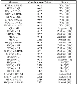
Table 2.10: Some correlation coefficients between different length measures.

Measures Correlation coefficient Source STPL v. 2.5% SL

STPL v. UQL UQL v. 2.5% SL

STPL v. UHML STPL v. UQL STPL v. 3.0% SL

UQL v. 3.1% SL UHML v. 3.1% SL

UQL v. ML UHML v. UI UHML v. ML

ML v. UI ML v. UI SFC(n) v. UHML

SFC(n) v. ML SFC(n) v. UI SFC(w) v. UHML

SFC(w) v. ML SFC(w) v. UI SFC(w) v. UI SFC(w) v. UI SFC(w) v. UR SFC(n) v. UI SFC(n) v. UR SFC(w) v. HVI-UI SFC(w) v. Fib.-UI ML v. 2.5% SL SFC(w) v. 2.5% SL

0.32 0.42 0.72 0.42 0.62 0.99 0.98 0.88 0.89 0.52 0.97 0.72 0.615 0.59 0.66 0.75 0.71 0.77 0.80 0.38 0.346 0.328 0.282 0.425 0.955 0.535 0.980 0.523 Woo [111] Woo [111] Woo [111] Woo [111] Woo [111] Woo [111] Woo [111] Woo [111] Bargeron [13] Zeidman [116] Zeidman [116] Zeidman [116] Prakash [81] Zeidman [116] Zeidman [116] Zeidman [116] Zeidman [116] Zeidman [116] Zeidman [116] Bargeron [11] Sief [93] Sief [93] Sief [93] Sief [93] Ramey [85] Ramey [85] Prakash [81] Prakash [81]

The measurement of individual fibers causes much of the trouble associated with

sample preparation. Short fibers have a tendency to cluster, so that their number in the

test sample is either too large or too small. Even severe fiber breakage has only a minor

influence on staple length but a major effect on percent short fiber content. Tallant, Fiori,

Alberson and Chapman [102] found that when various percentages of short fibers were

added to a base sample, there was no appreciable decrease in upper quartile lengths and

the change in the mean length was moderate. Hall [42] concluded that 50% span length

SFC have been developed on the basis of length uniformity and controversial results have

been found as can be seen from Table 2.10. The traditional Preysch formula derives SFC

from HVI measurements of two span lengths (equation 2.20):

(

)

(

)

SFC%=39.4+1.3× 2.5% −4.6× 50% Equation 2.20 Zeidman, Batra and Sasser [116] emphasized that Preysch predictions always

exceed the experimental values. They derived new equations for SFC which depend on

ML, UHML, and UI. The maximum coefficient of correlation was found to be 0.695.

Using two span lengths as in Preysch they obtained equation 2.21.

(

)

(

)

SFC%=50.01−0.766× 2.5% −81.48× 50% Equation 2.21

2.2. MEASUREMENT SYSTEMS

Fast and accurate single fiber measurements are desired characteristics of a

reliable fiber length measurement method. Subjective measurement of fiber length is

associated with inaccuracy especially when the classer is not familiar with the type of

cotton. Lack of familiarity with standards is another important source of inaccurate

results. One survey showed that there were wide differences in the assessment of length;

in extreme cases this difference could go up as much as 3/8 inch to ½ inch between two

classers [68].

Objective methods were designed to eliminate these personal differences in staple

length determination. The comb sorter is one of the earliest designs of the

semi-mechanical length measurement device. Baer Sorter and Suter-Webb devices are the best

known types of the sorters. Suter-Webb was used in the US as a standard method. Hertel

the standard test method to officially measure all the US crop. The Spinlab-type HVI

uses the same approach as the Fibrograph method to measure fiber length. The MCI-type

HVI uses a pneumatic principle. The Peyer instrument is another important application of

fiber length measurement scanning of the whole sample length distribution. In late

1980’s, AFIS was introduced to measure the fiber length distribution and was the first to

directly measure SFC. All systems have their own advantages and disadvantages. Let us

look at these important systems more deeply.

2.2.1. Array Method

This method is acknowledged as the most accurate method available by ASTM

[2], with the exception of individually measuring a very large number of single fibers. It

has long been used to measure the complete fiber length distribution and the test results

are used as reference values for other methods. However, it is extremely time

consuming, costly, and requires skilled operators. It takes approximately 2-3 hours per

sample [10, 9] and sampling, testing method and skill of the operator influence the

results. Particularly for short fiber content, repeated measurements are necessary for

satisfactory accuracy in many applications [82]. The USDA charges $137 for each

sample using this method, while charging $38 for Peyer and $9.5 for Fibrograph [107].

In this method, a predetermined weight (75 mg) of fibers are sorted into common

length groups onto a velvet board in 0.125-inch intervals. The velvet board shows the

staple length distribution of the sample. Then, beginning with the longest group each

length group is weighed. Weight data are used to calculate mean length, upper quartile

length and other length measurements. A sample calculation is carried out by ASTM for

Table 2.11: Fiber length array method [2].

Length, L Lower limits

(in.) Group weights,W

Length squared, L2

Sum of weights Cumulative percentage of

fibers

23 1.375 4.0 529 4.0 5.31

21 1.250 11.6 441 15.6 20.74

19 1.125 18.9 361 34.5 45.88

17 1.000 13.2 289 47.7 63.43

15 0.875 9.0 225 56.7 75.40

13 0.750 5.1 169 61.8 82.18

11 0.625 3.8 121 65.6 87.23

9 0.500 1.7 81 67.3 89.49

7 0.375 3.2 49 70.5 93.75

5 0.250 2.3 25 72.8 96.81

3 0.125 1.6 9 74.4 98.94

1 0.000 0.8 1 75.2 100.00

Totals 75.2

=1217.0

WL WL2 =21583.2

A. Upper Quartile Length

1. Cumulative sum of longest group weights equal to or greater than quartile=34.5

2. Quartile W/4………=18.8

3. Difference (Line 1 minus Line2) ……….=15.7 4. Correction=Diff.x0.125/weight group containing UQL=15.7x0.125/18.9 =0.1038 in. 5. Lower limit of group containing UQL ……….=1.1250 in. 6. Upper Quartile Length (Line 4 plus Line 5)………..=1.2288 in.

B. Mean Length

Mean length= WL/

(

)

2 . 1203 0 . 1217 16 0 . 1217 = = × W in. C. Variance

1.

(

)

× = × 256 2 . 21583 256 / 2 W W

WL ………=1.121135 in.

2.

(

)

D. Standard Deviation

S.D.= Variance………...=0.313 in.

E. Coefficient of Variation

length Mean

100 S.D.×

With weight-length arrays, such as those obtained from Suter-Webb sorter, it is

common practice to calculate the average fiber length on a weight basis. This

automatically reduces the effects of variation in short fiber content, and as such, weighted

mean length varies more closely with staple length than mean length calculated on a

number base. The coefficient of variation from a length array gives some indication of

the relative amounts of long and short fibers present.

Zeidman, Suh, Batra and Sasser [117] emphasized that length groups are

contaminated by other shorter or longer length groups during the segregation process.

This affects the accuracy of all measurements, but especially the longest and shortest

length range. Since other groups have two adjacent length groups, the errors are diluted.

The shortest group has only one neighbor and after removing presumably all fibers longer

than 0.125 in., the remaining fibers are all assumed shorter than 0.125 in.

ASTM carried out an interlaboratory test to evaluate the accuracy of this method.

Table 2.12 shows the components of variance expressed as standard deviations.

Table 2.12: ASTM array interlaboratory test results [2].

Test item Single operator Within laboratory Between laboratories

UQL, in. 0.01905 0.00140 0.00623

ML, in. 0.02196 0.00227 0.01307

CV% 1.450 0.361 1.173

SFC 1.441 0.033 1.162

For the components of variance in Table 2.12, the averages of observed values for

both the three specimen and the two specimen tests should be considered significantly

different at the 95% probability level if the differences equal or exceed the critical

Table 2.13: ASTM 95% confidence interval significant levels [2].

Number of specimens in test

and item

Single operator Within laboratory Between laboratories

Three specimen test

UQL, in. 0.030 0.031 0.035

ML, in. 0.035 0.036 0.051

CV% 2.3 2.5 4.1

SFC 2.3 2.3 4.0

Two specimen test

UQL, in. 0.037 0.038 0.041

ML, in. 0.043 0.043 0.057

CV% 2.8 3.0 4.4

SFC 2.8 2.8 4.3

2.2.2. Fibrograph

The original idea of the Fibrograph was developed by Hertel and Zervigon [45] in

1936. It was intended to plot a seed cotton staple diagram by scanning the entire

distribution of the sample. Hertel [46] developed the fibrogram theory that random

caught fibers configure the fibrogram curve if they are arranged with their catching points

along the vertical axis. Later the Fibrograph was digitized and added new features such

as 2.5% SL, 50% SL and UR.

The Fibrograph simply scans caught fibers from the starting point to some

maximum distance (no more fibers) while measuring the transmitted light intensity at

each measurement point. Any variation in the number of fibers varies the amount of light

detected. The 2.5% span length, 50% span length and uniformity ratio are derived from

these data [3].

The Fibrograph is subject to a number of error sources. Krowicki and

Thibodeaux [58], and Krowicki, Hemstreet and Duckett [61] reported important error

sources to include: fiber crimp, lack of random clamping, starting of the scan relative to

holding length of the sampler as 4.06 mm. Taking the average start of scan as 3.81 mm

and adding the average holding length, they found the actual beginning scan distance as

7.87 mm. Considering fiber crimp in addition to the combined effect of average holding

length and beginning scan distance, they found an average ratio of 1.2 for the theoretical

to measured length of upper half mean length and 2.5% span length.

Depending on the desired precision, two or four specimens from each subsample

are tested. ASTM carried out an interlaboratory test in which two operators in each of

three laboratories performed fiber length tests. The components of variance calculated

from the results of these tests an expressed as standard deviations are listed in Table 2.14.

Table 2.14: Components of variance of Fibrograph calculated from two specimen test results and expressed as standard Deviations [3].

Test item Single operator Within laboratory Between laboratories 2.5% SL, in. (mm) 0.01163(0.295402) 0.00003(0.000762) 0.00360(0.09144) 50% SL, in. (mm) 0.01028(0.261112) 0.00137(0.034798) 0.00834(0.211836)

50/2.5 UR, % 1.270 0.117 0.973

For the components of variance in Table 2.14, the averages of observed values for

both the four specimen and the two specimen tests should be considered significantly

different at the 95% probability level if the differences equal or exceed the critical

differences in Table 2.15.

Table 2.15: Critical differences between two means in cotton fiber length tests [3].

Number of specimens in test

and item

Single operator Within laboratory Between laboratories

Four specimen test

2.5% SL, in. (mm) 0.016(0.4064) 0.016(0.4064) 0.019(0.4826) 50% SL, in. (mm) 0.014(0.3556) 0.015(0.381) 0.027(0.6858)

50/2.5 UR, % 1.8 1.8 3.2

Two specimen test

2.5% SL, in. (mm) 0.023(0.5842) 0.023(0.5842) 0.025(0.635) 50% SL, in. (mm) 0.020(0.508) 0.021(0.5334) 0.031(0.7874)

2.2.3. HVI-Spinlab

HVI-Spinlab uses the same principle of the Fibrograph for length measurement

and includes other features, such as micronaire, strength, and elongation testing. It is the

official USDA method that every bale in the US is measured by HVI. However, like all

other methods they are subject to error.

Holding length is one of the important error sources whenever a holding device is

used in scanning fibers to determine length parameters. Holding length is about 0.16 in.

With the start of scan set point at 0.15 inch to 0.20 inch from the held point [87, 115],

total unmeasured length is about 0.31 in. According to Zeidman and Batra [115] mostly

short fibers are affected in this unmeasured area. On the other hand, the proportion of

shorter fibers is smaller and that of longer fibers is larger in the sample than in the

population. Thus, sampling error influences the short fiber content to a much higher

degree than the long fibers.

A lens system that is about 0.125 inches wide scans caught fibers from the

starting point to some maximum distance while measuring the transmitted light intensity

[87]. The fibrogram is influenced by all fibers in the optical system. In the region of

longer fibers, the rate of change is small and the actual optical reading approximates the

mathematical average of the mass over the detector width of 0.125 inches. However, this

is not true at the start of the fibrogram. This effect is referred to as lens broadening.

Palmer, Cooper, Pellow, McRae and Anderson [75] claimed that the Uniformity

Index of Spinlab was similar to Fibrograph, while the mean length of Spinlab was

consistently about one thirty-second of an inch shorter than Fibrograph measurements.

between Spinlab and Fibrograph and the correlation coefficient of the SFC 0.949 between

Spinlab and Suter-Webb. Table 2.16 shows the components of variance and 95%

probability level critical differences of ASTM test [4].

Table 2.16: Components of variance and critical differences of HVI-Spinlab [4].

Standard deviations in indicated

units Critical differences in indicated unitsTwo-specimen test Within lab. Between lab. Within lab. Between lab.

UHML, inch 0.013 0.030 0.035 0.091

UI, % 1.00 1.53 2.78 5.07

2.2.4. HVI-MCI

Brown [17] introduced the earlier version of pneumatic fiber length measurement.

In this method, the length analyzer determines length parameters of the test beard by

pneumatically scanning the specimen. Instead of using light, this system measures the air

pressure drop across an orifice as the specimen is passed through the orifice. The

pressure drop across the orifice is proportional to the total specific area of fibers in the

orifice. Assuming that the fibers are uniform in cross section or specific area, the

pressure drop is a measure of the number fibers in the air flow path. Therefore, as the

specimen is being raised from the orifice, the pressure drop profile gives a measure of the

number of fibers at each point along the length of the specimen. By scaling the output

pressure from shortest distance to maximum distance, the specimen is converted into an

internal representation of the percentage of the total number of fibers present at each

length value.

Associated errors of the MCI method are similar to Spinlab. The average holding

length is 0.11 inch and its start of scan is set at 0.20 inch so that the total unmeasured

Hemstreet and Thibodeaux [59], MCI measures all lengths 0.05 inch longer than Spinlab.

The correlation coefficient of the Upper Half Mean Length, the Uniformity index and the

Mean length of MCI and Suter-Webb array method have been found to be 0.914, 0.562,

0.871 respectively [117].

Gourlot, Vialle, Lassus, Duplan, Brunissen and Fallet [39] studied the effect of

the pinch and universal sampling methods on accuracy. In the pinch sampler, a

mechanical arm presses the pinch into the fiber mass. The pinch closes to hold the fibers

which are then separated from the sample when the mechanical arm withdraws. In the

universal sample, a comb removes fibers through perforations in a metal plate. A

mechanical arm carrying the pinch presses it against the fiber mass. The pinch closes to

hold the fibers which are then separated from the sample. Combing and brushing take

place after pinching. Chanselme, Gourlot and Tamime [20] studied the universal and

fibrosampling methods. In the Fibrosampler, fibers are combed before pinching. Results

showed significant differences in the distribution and accuracy of length measurements.

Table 2.17 shows components of variance and 95% probability level critical differences

of ASTM test D 4604-95 for the HVI-MCI method [5].

Table 2.17: Components of variance and critical differences of HVI-MCI [5].

Standard deviations in indicated

units Critical differences in indicated unitsFour-specimen test Within lab. Between lab. Within lab. Between lab.

UHML, inch 0.016 0.021 0.044 0.073

UI, % 0.87 0.89 2.41 3.44

2.2.5. Peyer ALmeter

The Peyer texlab system, developed for measuring the length of wool, appears to

The Peyer comprises two systems which sort and align a fiber bundle and measure its

length distribution. The Fibroliner (FL-101) mechanically combs either sliver or ginned

lint specimens into a parallel bundle or beard. The aligned fibers are placed between a

pair of carrier films for measurement. The ALmeter (AL-101) scans the beard using

capacitance measurements to produce an output signal that is proportional to the

cumulative mass distribution. The capacitor scans the fibers of the test specimen every

0.125-mm (0.005-in.). The microprocessor can convert the mass distribution to a number

distribution when the linear density of the fibers is assumed to be constant.

It takes about 15 minutes to test a sample on the Peyer ALmeter. The ALmeter

can produce at least six different sets of array information from the raw data, including a

fiber mass distribution, a number distribution, a fibrogram, and parametric values such as

mean length and upper half mean length by weight and by number, the variance, and the

25% and 50% span lengths.

Hemstreet and Krowicki [44] measured the fiber length and length distributions

for different staple length cottons using the Peyer system. Table 2.18 shows that the

mean length by weight for the measured distributions appears shorter than the known

distribution. The UHML and the UQL appears longer for the input than for the measured

distribution. They observed that SFC by number is significantly lower than the known

percentage. The weight loss that occurred in the samples ranged from 4 to 7% of the

original sample. This percentage loss by number appears to increase with the length of

the variety. Cui et al. [25] observed an average 1.20% short fiber loss and an average of

4.75% long fiber loss, and the ratio of short fiber loss to total loss was 23.60% for the

Table 2.18: Peyer length measurement comparison [44].

Type I Type II Type III

known Peyer known Peyer Known Peyer

ML(n), in. UHML(n), in. UI, % SFC(n), % ML(w), in. UQL, in SFC(w), % 0.757 1.009 75.0 17.7% 0.862 1.016 5.9% 0.753 0.975 77.2 14.7% 0.822 0.990 7.5% 0.810 1.165 69.5 23.3% 0.971 1.175 7.8% 0.815 1.121 72.7 16.7% 0.920 1.139 7.6% 0.928 1.557 59.6 25.3% 1.223 1.573 6.6% 0.970 1.467 66.1 16.1% 1.160 1.496 6.0%

Bargeron [11] compared the Peyer with the Suter-Webb array method. The

average difference between the Peyer 25% and Suter-Webb UQL was -2.40 mm with a

standard deviation of 0.86 mm. The linear correlation coefficient between the two was

0.99. The average difference in ML was –1.37 mm with a standard deviation of 1.02

mm. The linear correlation coefficient between the Suter-Webb ML and the Peyer was

0.99. SFC was greater than the Suter-Webb with an average difference of +1.70%, and a

standard deviation of 2.40%. Ramey and Beaton [85] found a 0.961 correlation

coefficient of SFC between the Peyer and Suter-Webb. Another analysis of Bargeron

[13] showed 0.87 correlation coefficient of the ML between the Peyer and Suter-Webb.

He explains the differences in the Suter-Webb and the Peyer distributions with the crimp

factor. Table 2.19 gives the variance components of Peyer according to ASTM [6].

Table 2.19: Variance components of Peyer [6].

Test item Within Laboratory Between laboratories ML, in. (mm)

UQL, in. (mm) CV (%) SFC, % 0.0193(0.490) 0.0224(0.569) 2.06 2.20 0.0208(0.528) 0.0244(0.620) 2.2071 2.4166 2.2.6. AFIS

opening and carding, followed by electro-optical sensing. The fibers are separated from

microdust and trash, and opened using specially designed pinned and perforated cylinders

and stationary carding flats [1]. Airflow into the perforations of the cylinder allows

efficient dust and trash removal by the combination of combing via the stationary carding

flat and the airflow drawn through the cylinder[1]. Each of the components is transported

in separate pneumatic paths to be analyzed electro-optically as in Figure 2.9.

Figure 2.9: AFIS fiber individualizer [1].

The Electro-optical sensor consists of three basic elements: tapered entrance and

exit nozzles, beam-forming and collecting optics, and the detection circuitry (Figure

2.10). Individual fibers are transported pneumatically from the fiber individualizer by a

high-velocity air stream. As the material enters the tapered nozzle, it is accelerated and

collimated beam of light. The fibers scatter and block that light in proportion to their

mean optical diameter and in direct relation to their time of flight through the beam [1].

Figure 2.10: Electro-optical sensor [1].

There are a number of error sources in AFIS measurements. There are fiber

breakages in the opening unit between 1% to 4% [26]. Fiber straightening, separation

and alignments are questionable. Only between 9% to 33% of fibers are counted in the

measurement unit [26], therefore there could be a bias for longer or shorter fiber lengths.

Cui, Calamari and Krowicki [26] established a test method to measure AFIS

accuracy. The same number of different known lengths, 0.25, 0.50, 0.75, 1.00 and 1.25

inch, acrylic fibers were tested on AFIS. The percentage of each fiber length group was

measured by AFIS as shown in Table 2.20. They also observed that lower sample density

increased the percentage of fibers counted, while higher density reduced testing time.

The length measured was not affected significantly based on the densities and samples

used. The correlation coefficient between the results from the AFIS and HVI systems is

Table 2.20: AFIS length accuracy test [26].

Cut length

(in) Measured length(in) Percentage inSample (%) Percentage Counted (%) 0.25 0.50 0.75 1.00 1.25 0.28 0.57 0.80 1.04 1.18 20 20 20 20 20 19 23 25 18 15

Cecil [19] studied the repeatability and the variation from test to test within the

AFIS. The AFIS has produced significant amount of variation from run to run. In this

study there were larger variations from run to run than between gins and farmers, and this

variation questions the ability of the AFIS to produce accurate results.

Table 2.21: AFIS measurement variability on SFC and UQL [19].

SFC (%) Run# (10,000

fibers) Min. Value Max. Value

1 4.8 7.4

2 8.9 12.4

3 10 13.4

UQL (in) Run# (10,000

fibers) Min. Value Max. Value

1 1.13 1.23

2 1.17 1.27

3 1.08 1.16

Cecil [19] conducted further tests with known 1.25-inch staple length polyester

samples. The mean length by weight was measured to be 1.1 inches, and by length to be

1.03 inches. SFC values for the polyester samples averaged 0.6 percent by weight and

2.1 percent by number with a maximum of 4.4 percent by number for one sample tested.

Over 70% (by weight) of the fibers were measured to be shorter than the 1.25 inch given

polyester staple length. Cecil also found that sample density significantly affected SFC

On the other hand, other researchers found controversies regarding the accuracy

of the AFIS as in Table 2.22 and Table 2.23. Cui , Calamari, Robert and Watson [25]

found the repeatability of SFC of AFIS 0.745 for bales and 0.8399 for slivers.

Table 2.22: Some correlation coefficients of AFIS versus Suter-Webb.

Suter-Webb v. AFIS Correlation coefficient source ML UQL SFC ML UQL SFC 0.96 0.96 0.89 0.98 0.98 0.98 Bragg [15] Bragg [15] Bragg [15] Ghorashi [38] Ghorashi [38] Ghorashi [38]

Table 2.23: 28 Staple length expected and measured values [87].

Length Data Expected Suter-Webb AFIS ML(w) ML(w) CV% SFC(w) UQL(w) ML(n) ML(n) CV% SFC(n) UQL(n) 0.82 23.7 6.6 0.96 0.75 29.9 14.2 0.92 0.75 29.9 14.2 0.92 0.63 44.7 31.6 0.84 0.75 32.7 13.6 0.89 0.64 43.1 28.7 0.81

Guse, Scheffer, Tabibi and Tauber [41] added two new features to the AFIS

principal measurement method, namely the fiber velocity tester and a multi-diode linear

camera called ITV. Measured length depends not only on time but velocity, too. AFIS

supposes that all fibers have the same velocity in the airstream. The multi-diode camera

detects when two or more fibers appear simultaneously in the measuring window and

omits them from measurement. The mean length measured on the basis of number of

fibers were found to be 19.0 mm for 20-mm fibers, 13.5 mm for the 15-mm fibers, and

9.5 mm for 10-mm fibers. Additionally, they found that the ITV, AFIS and Peyer

showed the same trend in mean fiber length, with the Almeter and the ITV giving about

2.2.7. Conclusion

Each system has its own inherent advantages and disadvantages. Longer length

measurement values are generally highly correlated to each other and usually satisfactory

results can be obtained. However, short fiber content measurement is not satisfactory.

None of the existing systems is able of measuring the short fiber content accurately. HVI

and Fibrograph methods cannot scan lengths less than about 0.31 inch. The Peyer

method losses many fibers in the opening unit resulting in a change in fiber length

distribution. AFIS appears to be the ideal method with single fiber length measurement;

however, there are considerable controversies about its accuracy and repeatability. More

accurate measurement of cotton fiber length and length distribution is needed and

recently being driven by the industry.

Table 2.24 compares UQL, ML, and SFC values as measured by Array, AFIS,

Peyer and HVI length measurement systems on standard cotton types. Table 2.25 shows

correlation coefficients between measurement systems according to Smith and Williams

[94].

Table 2.24: UQL, ML, and SFC comparisons of length measurement systems [94].

Array AFIS Peyer HVI

Staple

length UQL ML SFC UQL ML SFC UQL ML SFC UQL ML SFC