Development of a Nonlinear Time Domain Methodology (Part I)
Justin Coleman
1, Robert Spears
2, and Mike Cohen
31
Seismic Engineer, Idaho National Laboratory, Idaho Falls, ID ([email protected]), USA
2
Seismic Engineer, Idaho National Laboratory, Idaho Falls, ID ([email protected]), USA
3
Mechanical Engineer, TerraPower, Bellevue, WA, ([email protected]), USA
ABSTRACT
The ASCE 4-2014 (draft) provides guidance in Appendix B for nonlinear time-domain soil structure
interaction (NLSSI) analysis. To accommodate widespread use of NLSSI, it is necessary to develop a
methodology, or a set of steps, that produce reasonable results. An NLSSI methodology opens the door
to explore additional seismic behaviour at nuclear facilities such as 1) gapping and sliding, 2) inclined
seismic waves coupled with gapping and sliding of foundations atop soil, 3) inclined seismic waves
coupled with gapping and sliding of deeply embedded structures, 4) soil dilatancy, 5) surface waves, 4)
buoyancy, 5) concrete cracking and 6) seismic isolation. This paper documents the NLSSI methodology.
At a high level these steps include 1) define soil site parameters, 2) calibrate site-specific nonlinear soil
constitutive model, 3) verify performance of time domain absorbing boundaries, 4) build free field soil
site, 5) build 3D soil site model using the appropriate parameters 6) define design concrete material
properties and develop appropriate concrete constitutive model, 7) build structural model, 8) define
appropriate contact and/or friction behaviour, 9) build combined soil-structure model and run time
domain models and 10) compare with SHAKE/SASSI results at increasing levels of ground motion. This
paper will describe the NLSSI methodology, discuss important NLSSI considerations, and discuss its
potential implementation in industry. A second paper, which is Part II, “Development of a Nonlinear
Time Domain Methodology Results,” provides results comparing in-structure response from NLSSI with
the linear frequency-domain program, SASSI.
INTRODUCTION
The Department of Energy (DOE) and the nuclear industry currently performs seismic soil-structure
interaction (SSI) analysis of existing and new nuclear facilities using equivalent-linear numerical analysis
tools. These tools approximate the nonlinear response of the soil and the structure, and involve modeling
of the soil-foundation interface using rudimentary procedures. Equivalent-linear tools are expected to
produce reasonable estimates of in-structure response for lower levels of earthquake ground motion
intensities that result in low strains and almost linear soil and structural response. For higher levels of
ground motion intensities for which, the soil strains are high and gapping and sliding at the
soil-foundation interface is likely, these tools are likely inaccurate.
The estimate of the seismic hazard at nuclear facilities continues to evolve and generally leads to an
increase in the hazard. The change in understanding of the site-specific seismic hazard curve occurs as
more information is gathered on seismic sources and events, and additional research is performed to
update attenuation relationships and characterize local site effects. As the seismic hazard increases, more
intense input ground motions are used to numerically evaluate nuclear facility response. This results in
higher soil strains, increased potential for gapping and sliding and larger in-structure responses.
Therefore, as the intensity of ground motions increases, the importance of capturing nonlinear effects in
numerical SSI models increases.
nonlinear time domain numerical codes. The methodology is herein termed Nonlinear Soil-Structure
Interaction (NLSSI).
This paper will describe the NLSSI methodology by Spears and Coleman (2014), and discusses
important NLSSI considerations, and its potential implementation in industry. A second paper, which is
Part II, “Development of a Nonlinear Time Domain Methodology Results,” provides results comparing
in-structure response of NLSSI with SASSI (
Lysmer, et. al.
1999)
.
NLSSI METHODOLOGY DEVELOPMENT
Numerical tools for performing NLSSI analysis in the time domain are available. However, using
these tools can be complicated and requires a standardized methodology that can be followed by analysts
and researchers. The NLSSI methodology is a series of steps that the analyst can perform to produce
reasonable results using any time-domain code. Figure 1 of the paper outlines these steps. The NLSSI
methodology also creates an opportunity to explore more seismically-induced phenomena at nuclear
facilities, which include the following: 1) gapping and sliding, 2) inclined seismic waves coupled with
gapping and sliding of foundations atop soil, 3) inclined seismic waves coupled with gapping and sliding
of deeply embedded structures, 4) soil dilatancy, 5) surface waves, 4) buoyancy, 5) concrete cracking and
6) seismic isolation. The NLSSI methodology presented in this paper is developed for vertically
propagating shear waves, gapping and sliding of the foundation, and soil nonlinearity. Future research
will focus on developing verified and validated methods and numerical tools for addressing additional
seismically-induced phenomena presented above. To build confidence in the NLSSI methodology
presented here-in, the results have been benchmarked by comparing the results of NLSSI analyses with
those from a recently verified and validated version of the frequency-domain, linear analysis code SASSI
(System for Analysis of Soil-Structure Interaction).
At low intensities of input ground motion, the linear analysis and NLSSI should produce similar
results. For higher intensities of input ground motion, the results from linear and NLSSI analyses are
expected to diverge due to gapping and sliding and/or soil nonlinearity. The details of the methodology
are presented below, results from a case study using a generic nuclear power plant (NPP) are provided in
Development of a Nonlinear Time Domain Methodology, Results (Part II).
METHODOLOGY
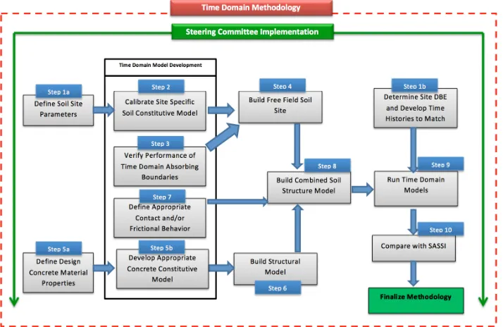
The process for performing NLSSI and developing a time-domain methodology is presented in
Figure 1. This figure identifies specific steps that are important to producing reasonable NLSSI results.
The methodology was developed by performing hand calculations and linear analysis (SASSI) and
comparing with NLSSI results. For this development effort the explicit solver in LS-DYNA (LSTC
2013) was mainly used with results also calculated using ABAQUS (Dassault Système’s 2012) implicit
and explicit solvers.
Spears and Coleman
2014 provides additional information for each of the steps
listed below.
•
Step 1a: Define soil site parameters
o
Characterization of site-specific soil properties is an important first step when performing any SSI
analysis (linear or NLSSI).
o
Define the site-specific soil layers: Site-specific soil layers need to be defined from the location
of definition of rock outcrop motion to the surface.
o
Determine G/Gmax and Damping vs. Shear Strain Curves: Site-specific soil data can be gathered
and experimental tests run (torsional shear tests or resonant column tests) to determine dynamic
soil properties at various soil depths.
o
Determine soil density and elastic mechanical properties
•
Step 1b: Determine the design basis earthquake (DBE) for the site and develop spectrally matched
input ground motions
o
When performing NLSSI analysis it is desirable to have the ground motion defined at rock
outcrop. This is because to perform NLSSI analysis it is necessary to develop three dimensional
force time histories to be applied to the numerical finite element model. The NLSSI time domain
approach accounts for the inertial effects of the soil column. Therefore there is no need to
attenuate the motion up to the surface and deconvolve down to develop inlayer motion.
o
Using rock outcrop motion to define force time histories that will be applied at depth.
•
Step 2: Calibrate the nonlinear hysteretic kinematic hardening soil constitutive model using
site-specific soil properties
o
Use the site-specific dynamic soil property data developed in Step 1a (G/Gmax and damping
versus shear strain curves) to calibrate the NLSSI model and match the energy dissipated
(hysteretic behaviour) by the theoretical SHAKE equations using one element model. This
allows for realistic dissipation of energy in soil, frictional dissipation and reduction in soil
stiffness. As opposed to the current approach (used in equivalent linear analysis) for energy
dissipation, using frequency independent damping related to viscous dissipation.
o
Demonstrate that a multi-layered soil site, using the time histories developed in Step 1b, produces
similar surface response when analysed using SHAKE and the NLSSI approach
•
Step 3: Verify performance of absorbing boundaries in the time domain
Absorbing boundary conditions are needed in a time domain analysis to remove any reflected or
radiated waves from the local soil domain. The methodology presented in this paper considers
vertically propagating shear waves, which requires absorbing boundary conditions on the bottom of
the soil domain and boundary constraints along the sides of the soil model that allow nodes to move
together. This approach does not require absorbing boundary conditions along the vertical faces of
the soil domain, but it does require the modeled soil domain to be sufficiently large.
change the ISRS. To demonstrate the appropriate size of soil domain has been select the analyst
should compare 2x, 3x, and 4x building width soil mesh and track the sensitivity of ISRS. An
example of these calculations if presented later in this paper. It is likely that the potential impact
on ISRS will occur when the nonlinear soil remains elastic. The reason for this is that for larger
levels of shaking will produce increased soil nonlinearity, and this increased soil nonlinearity will
absorb energy as it radiates away from the structure.
o
Compare the NLSSI in-structure response with SASSI at 0.5*DBE and low levels of soil
damping. The reason for the low level of soil damping and the low level of shaking (0.5*DBE) is
that the localized nonlinear area of influence around the structure is greatly decreased and the
waves (energy) radiated away from the structure will not be dissipated. This is a great test of
waves potentially reflecting off the boundaries and changing ISRS.
•
Step 4: Build a free-field soil site
o
Build three-dimensional soil site model using the information generated in Step 1, appropriate
soil parameters developed in Step 2.
o
Model appropriate boundary conditions as defined in Step 3.
o
Verify that the vertically propagating shear wave, three-dimensional, time-domain, free-field
NLSSI site response matches the responses calculated using one-dimensional analysis using
SHAKE and one-dimensional nonlinear site response analysis.
o
Test the three-dimensional soil site using the appropriate time histories
•
Step 5a and 5b: Define design material properties for concrete and calibrate an appropriate
constitutive model
o
When using elastic concrete material properties this section is relatively straightforward. Elastic
concrete properties are used along with appropriate Rayleigh damping parameters tuned to the
frequency range of interest.
o
If nonlinear hysteretic kinematic hardening concrete constitutive models are used this step is
more complex and will require comparison of numerical concrete behaviour with experimental
tests.
•
Step 6: Build and verify the dynamic response of the structural model
o
Perform a base modal analysis to determine structural natural frequencies, and then a
fixed-base time-history analysis by subjecting the same model to site-specific three dimensional design
basis ground motions. Verify that the frequency content of the global structural response
reasonably correlates to the results of the modal analysis.
•
Step 7: Define appropriate contact and/or friction models:
o
Gapping and sliding can be modelled in the time-domain using two approaches: (1) a nonlinear
soil constitutive model that allows for changes in hydrostatic pressure, and has shear failure
criteria that allows for soil failure (sliding) in the soil elements, (2) a contact algorithm (penalty,
kinematic) to model gapping and sliding. The model used to test this methodology used the
second approach. However, significant effort was put into the first approach, which seems
feasible and likely desirable.
•
Step 8 and Step 9: Build combined soil-structure model and run time-domain models:
o
Verify that the combined model behaviour is reasonable by comparing initial results to the
fixed-base modal analysis, free-field model response, and other numerical codes (such as SASSI).
•
Step 10: Compare the responses from NLSSI analyses with those from SASSI analyses. Results from
development of NLSSI methodology are presented in “Development of a Nonlinear Time Domain
Methodology, Results (Part II).”
IMPORTANT NLSSI CONSIDERATIONS
Three important considerations when performing NLSSI are, appropriate soil site response,
appropriate absorbing boundary conditions, and appropriate size of finite soil domain. These three
considerations are discussed in more detail below with examples and results presented on how to
determine if an appropriate NLSSI model has been developed.
NLSSI SOIL SITE RESPONSE
To develop an NLSSI soil column that is
appropriate for modeling vertically propagating shear
waves, it is necessary to compare site-response results
with accepted equivalent linear numerical tools such as
SHAKE (Deng, N. and Ostadan, F, 2000). Bolisetti,
C. et. al (2014) present a comparison between
equivalent-linear and nonlinear (LS-DYNA)
site-response analysis at various U.S. soil sites. The
research presents an approach for modeling nonlinear
soil columns in nonlinear time-domain codes.
Independent of Bolisetti, C. et. al (2014), a method for
performing nonlinear site-response analysis for
implementation into a 3D SSI model was developed
by the Idaho National Laboratory (Spears and
Coleman 2014). Both Bolisetti, C. et. al (2014) and
Spears and Coleman (2014) independently confirm the
capability for performing site-response analysis for
vertically propagating shear waves.
The calculation approaches used by time-domain
codes and equivalent-linear codes such as SHAKE are mathematically different. Explicit time-domain
numerical tools step through time without performing numerical iterations, and update the stiffness of
each element at each time step. Frequency-domain numerical tools such as SHAKE, employ an iterative
process to select a stiffness and damping ratio for each soil layer that are compatible with the strain levels
observed for a given seismic loading. While the nonlinear, time-domain approach is more realistic, the
SHAKE approach is supported by several years of research and its results are generally accepted.
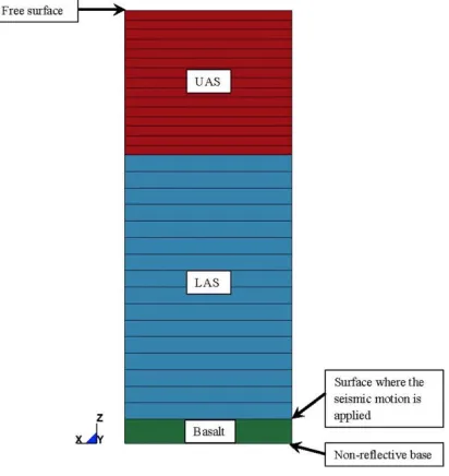
An example of verifying the performance of NLSSI soil column by comparing with SHAKE is provided
below. The soil column model used in this example is shown in Figure 3 and consists of 30-ft of upper
alluvial soil (UAS), 55-ft of lower alluvial soil (LAS) and 5-ft of basalt. Soil element thicknesses were
selected to pass a 40-Hz shear or compressive wave (linear solid elements were used therefore at least
10 elements per wave length are needed). The calculation for soil thickness should consider stiffness
reduction of the soil elements. The elements used in this example are 2-ft thick for the UAS, 3.44-ft thick
for the LAS, and 5-ft thick for the basalt. The boundary conditions applied to the soil column if Figure 3
are constraining at each elevation to translate together and absorbing boundary conditions (Non-reflective
base) applied to the basalt. These constraints simulate a soil domain that is infinitely horizontal.
Transfer Function Amplitude versus Frequency
Soil Column Depth versus Maximum Shear Strain
10 20 0 2 4 6 8 f T ra n sf er F u n ct io n A m p li tu d e Frequency [Hz]
Top-of-Soil Response Spectra versus Frequency
0.1 1 10 100
0 0.2 0.4
〈 〉
0 2 10× −5 4 10× −5
80 − 60 − 40 − 20 − 0 1 1
x y,
A cc el er at io n [ g ] Frequency [Hz] D ep th [ ft ]
Shear Strain [ft/ft]
Figure 4: Seismic soil column NLSSI results (green, cyan, and red solid curves) and SHAKE results
ABSORBING BOUNDARY CONDITIONS
Performance of absorbing boundary conditions is a
critical feature of NLSSI analysis. This is because
NLSSI models an essentially infinite soil domain as
finite. An appropriate demonstration of 3D absorbing
boundary conditions can be demonstrated by
developing a soil block and applying an edge load. To
determine if the numerical code can analyze 3D
inclined waves it is necessary to demonstrate that the
wave field remains reasonable and spurious (reflected
waves of the boundary) waves are minimized. To
demonstrate appropriate wave propagation a model
was developed and run using a NLSSI numerical tool.
The model shown in Figure 8 is a cube composed
of 1,000,000 uniformly sized, linear elastic elements
with soil material properties that are representative of
basalt. The cube has 100 elements per edge and an
edge length of 1000 ft. The model 1) has a free
boundary on the positive Z-direction surface, 2) is
restrained in the direction on the negative
Y-direction surface (for symmetry) 3) is restrained in the
X-direction on the negative X-direction surface (for
symmetry) and 4) the other three surfaces have a
non-reflecting boundary condition defined. The input
motion is a wavelet at the corner of the model
indicated in Figure 5.
A second analysis was performed that is identical
to that of the first, except that the three surfaces with
non-reflecting boundary conditions are now fixed,
namely, restrained in the X, Y, and Z directions.
Figures 8 shows contour plots of von Mises stress
resulting from the input wavelet. The stress range for
the contours is adjusted to show only the dominant
waves, but not the small reflections from the boundary
surfaces. The stress waves resulting from the input
wavelet motion should travel outward and leave the
model, in case of the model with non-reflecting
boundary surfaces. In the model with fixed boundaries,
the wavelets should reflect back and not leave the
model. This study shows that the non-reflecting
boundary conditions work as required, even for
inclined, three-dimensional wave propagation.
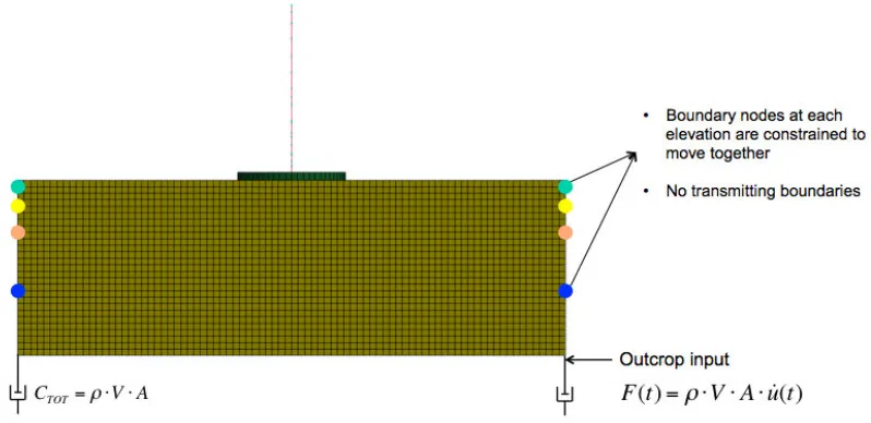
SIZE OF NLSSI FINITE SOIL DOMAIN
Performing NLSSI analysis using time domain codes
requires the analyst to limit the model size to a finite soil domain. A proper decision on the finite size of
the soil domain must be made so that ISRS results are not affected by spurious wave reflections off the
boundaries. The methodology here is specific to vertically propagating shear waves. To produce a
vertically propagating shear wave in time-domain the soil boundary nodes are constrained to translate
horizontally and vertically together. Using this constraint along the boundary may produce spurious ISRS
results. Therefore it is necessary to perform a sensitivity study to determine the size of the finite soil
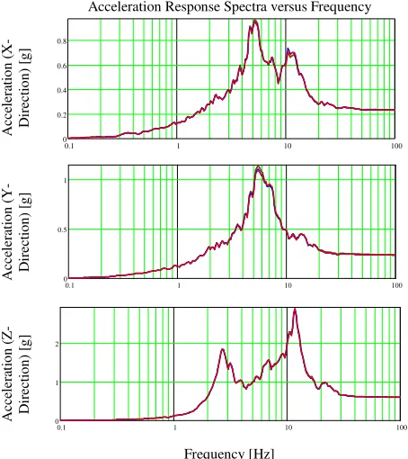
domain. The results presented below compare 2x, 3x, and 4x (Figure 6 shows an example of 4x for the
example problem) building width soil mesh and tracks the sensitivity of ISRS.
Acceleration Response Spectra versus Frequency
A cc el er at io n ( X -D ir ec ti o n ) [g ]
0.1 1 10 100
0 0.2 0.4 0.6 0.8 A cc el er at io n ( Y -D ir ec ti o n ) [g ]
0.1 1 10 100
0 0.5 1 A cc el er at io n ( Z -D ir ec ti o n ) [g ]
0.1 1 10 100
0 1 2
Frequency [Hz]