Bayesian Methods for Nonlinear and Discrete Data with Complex Dependence.

ABSTRACT

SINGH, SUSHEELA PATWARI. Bayesian Methods for Nonlinear and Discrete Data with Complex Dependence. (Under the direction of Dr. Brian J. Reich and Dr. Ana-Maria Staicu.)

Bayesian methods can be powerful tools for analyzing data with a variety of complex dependence structures. Hierarchical models are popular methods for analyzing data with dependence between observations, because they are flexible, seamlessly incorporate discrete data, and allow dependence to be specified in several layers, providing simple expressions for complicated marginal structures. When dependence occurs between model parameters rather than observations, commonly in nonlinear settings, Bayesian computational algorithms have been developed that can provide reliable samples from the posterior distribution for inference. In this dissertation, we consider both cases of dependence by developing two novel Bayesian hierarchical models for variable selection with application to high-dimensional, correlated data and then reviewing Markov chain Monte Carlo algorithms for estimating highly correlated parameters within a nonlinear regression framework.

First, we consider binary responses that are correlated both across the multivariate outcomes and spatially between observations. We develop a flexible Bayesian spike-and-slab variable selection model for presence-absence indicators that accounts for spatial dependence and cross-dependence between taxa, while reducing dimensionality in both directions. By simulation, we show that the proposed method improves variable selection, particularly for the low magnitude and low prevalence covariates that are of interest in the high-dimensional microbiome setting. We mirror the analysis of Barberán et al. (2015) and apply the proposed model and PERMANOVA, a popular distance-based method, to a fungal community found within household dust. We broadly corroborate their results that climatic and geographic variables are the main influences on fungal composition within homes, and we are able to provide additional detail about how the covariates influence individual taxa.

Second, we expand on the work of the initial model and propose analyzing ranks within samples rather than binary indicators. Ranking the outcomes within a sample simplifies comparison of composition between samples and can help to mitigate the effects of contaminated counts, while retaining structural information about the relationships between outcomes. We detail a Bayesian spike-and-slab variable selection model that is applicable to rankings of taxa derived from overdis-persed, contaminated, zero-inflated counts, and we specify an extended model that addresses multivariate correlation directly using random effects. We show by simulation that our proposed model outperforms a Bayesian model for the binary response and distance-based methods with a variety of responses in nearly all cases. Our method is applied to taxa found in the stool samples of healthy adults, and we find that very few of the analyzed covariates are identified as influencing microbiome composition.

© Copyright 2018 by Susheela Patwari Singh

Bayesian Methods for Nonlinear and Discrete Data with Complex Dependence

by

Susheela Patwari Singh

A dissertation submitted to the Graduate Faculty of North Carolina State University

in partial fulfillment of the requirements for the Degree of

Doctor of Philosophy

Statistics

Raleigh, North Carolina 2018

APPROVED BY:

Dr. Eric B. Laber Dr. Krishna J. Pacifici

Dr. Brian J. Reich

Co-chair of Advisory Committee

DEDICATION

BIOGRAPHY

ACKNOWLEDGEMENTS

First and foremost, I would like to thank my husband and partner in crime, Nikhil Singh, without whom I would be truly lost. Your humor, serenity, support, and unending patience have aided me when I needed it the most. You make me the best version of myself.

I’d also like to thank my advisors, Dr. Brian Reich and Dr. Ana-Maria Staicu, and my committee members, Dr. Eric Laber and Dr. Krishna Pacifici, for their invaluable guidance, teachings, and mentorship throughout this journey. I’ve been fortunate to have worked closely with Dr. Alyson Wilson, whose advice and understanding have righted my ship on more than one occasion. I am also grateful for the opportunities I’ve received to work with insightful collaborators including Drs. Rob Dunn, Ralph Smith, Jacob Jones, Noah Fierer, and Chris Fancher.

I am grateful to the faculty and staff in the Department of Statistics at North Carolina State University, who work incredibly hard to help prepare us to face the challenges ahead, be they academic or otherwise. In particular, I want to highlight and recognize Alison McCoy, who has been one of my biggest cheerleaders and a source of emotional support.

During my graduate studies, I have been lucky to develop wonderful friendships that provide an immensely strong foundation. Many, many thanks to Ali Miller, Meredith King, Katie Forster, Sam Morris, Kyle Roell, Matt Austin, Neal Grantham, and Eric Rose, in an inexhaustive, unordered list. You all, and others, have provided friendship, strength, levity, advice, and so much more.

TABLE OF CONTENTS

LIST OF TABLES . . . vii

LIST OF FIGURES. . . ix

Chapter 1 Introduction. . . 1

1.1 Variable selection for dependent, discrete microbiome data . . . 2

1.2 Posterior sampling for correlated parameter spaces . . . 4

Chapter 2 A Nonparametric Spatial Test to Identify Factors that Shape a Microbiome . . . 6

2.1 Introduction . . . 6

2.2 Motivating Data . . . 8

2.3 Nonparametric Spatial Model . . . 9

2.3.1 Identifying influential covariates . . . 10

2.3.2 Capturing residual dependence . . . 11

2.4 Estimating the spatial basis functions . . . 12

2.5 Simulation study . . . 14

2.5.1 Methods . . . 14

2.5.2 Results . . . 17

2.6 Data Analysis . . . 19

2.7 Discussion . . . 23

Chapter 3 Bayesian Variable Selection for High-Dimensional Rank Data. . . 25

3.1 Introduction . . . 25

3.2 Motivating Data . . . 27

3.3 Model . . . 28

3.3.1 Variable Selection . . . 29

3.3.2 Dependence Between Taxa . . . 29

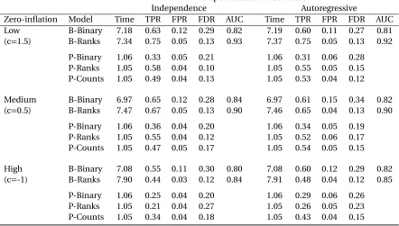
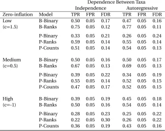
3.4 Simulation Study . . . 30

3.4.1 Methods . . . 30

3.4.2 Results . . . 33

3.5 Data Analysis . . . 34

3.6 Discussion . . . 37

Chapter 4 A Survey of MCMC Algorithms for Diffraction Pattern Analysis . . . 41

4.1 Introduction . . . 41

4.2 Rietveld Refinement . . . 44

4.2.1 Nonlinear Least Squares Algorithms . . . 45

4.2.2 Uncertainty Quantification . . . 47

4.2.3 Criteria of Fit . . . 48

4.3 Bayesian Approaches . . . 49

4.3.1 Metropolis Algorithm . . . 51

4.3.2 Joint Metropolis . . . 53

4.3.4 Approximate Bayesian Computing . . . 59

4.4 Discussion . . . 62

4.5 Summary . . . 65

BIBLIOGRAPHY . . . 68

APPENDICES . . . 77

Appendix A A Nonparametric Spatial Test to Identify Factors that Shape a Microbiome 78 A.1 Model properties . . . 78

A.2 Computing details . . . 80

Appendix B Bayesian Variable Selection for High-Dimensional Rank Data . . . 84

B.1 Identifiability of Parameters . . . 84

B.2 Computing Details for Base Model . . . 85

LIST OF TABLES

Table 2.1 Summary of true positive rate (TPR), false positive rate (FPR), and average model fitting time in minutes for PERMANOVA (PERM), the nonspatial (NS), parametric Mat´ern (Mat), and proposed nonparametric (SNP) models. . . 17 Table 2.2 Summary of “registered” true positive rate (TPR) and false positive rate (FPR)

for PERMANOVA (PERM), the nonspatial (NS), parametric Mat´ern (Mat), and proposed nonparametric (SNP) models. If values are not provided, there is no threshold value or significance level that controls the false positive rate at the required level. . . 18 Table 2.3 Inclusion rate for influential covariates for PERMANOVA (PERM), the

non-spatial (NS), parametric Mat´ern (Mat), and proposed nonparametric (SNP) models, broken out by covariate magnitude (S=Small, L=Large) and preva-lence (100%, 50%, 10%). . . 19 Table 2.4 Summary of variable selection results from PERMANOVA (PERM) and the

pro-posed spatial nonparametric method (SNP). P-values are reported from PERM, and the posterior probability of the null hypothesis, the expected number of taxa for which the covariate is included, and the number of taxa for which the coefficient value is positive or negative are reported for SNP. . . 21 Table 3.1 Summary of the abundance counts in a subset of the American Gut Project by

sex. . . 28 Table 3.2 Summary of average computing time in minutes, true positive rate (TPR),

false positive rate (FPR), false discovery rate (FDR), and area under the ROC curve (AUC) for the Bayesian binary variable selection model (B-Binary), the proposed Bayesian ranks variable selection model (B-Ranks), PERMANOVA with the binary response (P-Binary), ranks (P-Ranks), and the observed counts (P-Counts). . . 34 Table 3.3 Summary of true positive rate (TPR), false positive rate (FPR), and false

discov-ery rate (FDR) using the “registered” threshold to control overall FPR below 5% for the Bayesian binary variable selection model (B-Binary), the proposed Bayesian ranks variable selection model (B-Ranks), PERMANOVA with the bi-nary response (P-Bibi-nary), ranks (P-Ranks), and the observed counts (P-Counts). 35 Table 3.4 Summary of the P-values from PERMANOVA and the posterior mean

probabil-ity of the global null from the Bayesian models when applied to The American Gut Project data for females. . . 36 Table 3.5 Summary of the P-values from PERMANOVA and the posterior mean

probabil-ity of the global null from the Bayesian models when applied to The American Gut Project data for males. . . 37 Table 4.1 Prior bounds for the material and instrument parameters . . . 49 Table 4.2 Computation time and criteria of fit for the Bayesian algorithms presented in

Table 4.3 Estimated posterior mean and 95% credible interval (CI) for each parameter using each of the Bayesian algorithms from Section 4.3. . . 64 Table 4.4 Effective sample size (ESS) for each parameter using each of the MCMC

LIST OF FIGURES

Figure 2.1 Map of presence (purple circle) or absence (gray×) for two primarily indoor

fungal taxa at each sampling location. . . 9

Figure 2.2 Maps of the first four spatial basis functions estimated from the WLOH data. 20 Figure 2.3 Map of presence for taxa assigned to a large cluster of 100 taxa and a small cluster of 3 taxa. A darker point indicates that a higher number of taxa are present in a location. . . 22

Figure 3.1 Inclusion rates for influential covariates by prevalence (100%, 50%, 10%) and magnitude (L=Large, S=Small) for the Bayesian binary variable selection model Binary), the proposed Bayesian ranks variable selection model (B-Ranks), PERMANOVA with the binary response (P-Binary), ranks (P-(B-Ranks), and the observed counts (P-Counts). . . 39

Figure 3.2 Empirical cumulative density function for correlation between taxa in The American Gut Project data for the female and male subgroups, with the null distribution given in gray. . . 40

Figure 4.1 Angular dependent neutron diffraction profile from a NIST silicon standard reference material. . . 42

Figure 4.2 Trace plots for selected parameters from a one-at-a-time Metropolis sampler. 52 Figure 4.3 Scatter plot of posterior sampled values for the Caglioti parameters U and V using the one-at-a-time Metropolis sampler. The prior bounds for the param-eters are noted by dashed lines. . . 53

Figure 4.4 Trace plots for selected parameters using a joint Metropolis sampler. . . 54

Figure 4.5 Trace plots for selected parameters using the DRAM sampler. . . 56

Figure 4.6 Trace plots for selected parameters using the HMC sampler. . . 59

Figure 4.7 Difference curve and fitted profile from the DRAM algorithm applied to the neutron diffraction profile data. . . 63

Figure 4.8 Estimated posterior density for each parameter using each of the algorithms in Section 4.3. One-at-a-time Metropolis is a solid line, Joint Metropolis is a dashed line, DRAM is a dotted line, and ABC is dot-dashed line. The Rietveld estimate±2 e.s.d.’s is also given. . . 66

Figure 4.9 Pairwise scatter plots of the posterior samples for each of the instrument and material parameters of interest using the DRAM sampler. . . 67

CHAPTER

1

INTRODUCTION

Assumptions of independence upon which many statistical methods rely are often tenuous. De-pendence may creep into analyses in several ways, ranging from measurement errors to complex dependence between observations. Each of these sources poses its own particular challenges to analysis. In this dissertation, we will consider the challenges of modeling observations that exhibit correlation across space and multivariate outcomes and those of parameter estimation with depen-dence between model parameters. This chapter provides an introduction to, and a summary of, our contributions to the analysis of problems with complex dependence.

microbiome settings, while the third provides an alternative approach to an important problem in materials science that addresses many of the shortcomings of the current standard methodology.

1.1

Variable selection for dependent, discrete microbiome data

A microbiome is a diverse community of microorganisms (or microbes) such as fungi, bacteria, and viruses that occupy a specific ecological niche. These communities are found all over the planet, and interest in studying them has surged in the past few decades. With the development of high-throughput (or next-generation) sequencing technologies, the cost of studying these microbes via DNA material has steadily decreased. As a result of this newly accessible data, it is increasingly evident that microbial health plays a vital role in human health, with links to obesity and Crohn’s disease (Ley et al., 2005; Dicksved et al., 2008; Turnbaugh et al., 2009), Type 2 diabetes (Qin et al., 2012), allergies (Dannemiller et al., 2014), and immune system dysfunction (Round & Mazmanian, 2009), to name a few. However, much of the focus has centered on identifying and describing the effects of a microbiome on an outcome, with relatively less attention paid to the problem of identifying which external factors may influence the microbiome itself.

This is due, at least in part, to the fact that abundance counts (orreads) resulting from high-throughput sequencing pose a number of challenges for standard statistical analysis. First, the total number of sequencing reads is an artifact of the sequencing process and is not comparable across samples. Thus, abundance counts are compositional, and they relay relative information rather than absolute information. Second, the high-dimensional counts are frequently zero-inflated, overdispersed, and may be contaminated by errors in the sequencing process. Third, because the counts characterize a community, there may be dependence between the taxa that reflects underlying relationships. These characteristics complicate the application of multivariate statistical techniques.

information onhowa covariate may influence microbiome composition or which specific taxa may be affected.

In an effort to address some of these limitations, several parametric models have been developed for the abundance counts, including those based on the Dirichlet-multinomial (Chen & Li, 2013; Wadsworth et al., 2017), negative binomial (Zhang et al., 2017), or logistic normal multinomial distributions (Xia et al., 2013; Grantham et al., 2017). Nonparametric approaches to analyzing the abundance counts are not as common, but are available. Warton (2011) utilizes a generalized linear model framework to construct a permutation-based hypothesis test for covariate effects, and Zhao et al. (2015) takes a regression kernel approach. However, these models generally do not account for correlation between samples, and several rely on optimization routines that are not feasible for large problems.

Rather than analyzing counts that are compositional and may be noisy, practitioners frequently transform the data. Though merely considering relative taxa proportions instead of counts is not a full solution in itself, the literature proposes a suite of transformations of the relative taxa proportions (e.g., logratio transformation) that remove the compositional structure so that standard multivariate statistical methods may be applied appropriately (Aitchison, 1986; Fernandes et al., 2013; Mandal et al., 2015). Alternatively, the counts are commonly transformed to binary presence-absence indica-tors. Some of the aforementioned methods are applicable to binary data, such as the distance-based methods and Warton’s method, but they are subject to the same limitations. Shirota et al. (2017) develops a model that incorporates covariate information for presence-absence indicators, but its focus is on data fusion and prediction. Additionally, it does not account for dependence between samples or perform variable selection and testing.

In Chapter 2, we consider transforming to the multivariate binary response, which removes the compositional aspect of the data and reduces noise. We develop a nonparametric Bayesian hierarchical model with the goal of identifying covariates that influence microbiome composition while accounting for spatial dependence across samples and multivariate dependence between taxa. We show by simulation that in the presence of spatial dependence, the most popular distance-based hypothesis testing method (PERMANOVA) fails to preserve its advertised size, and the proposed model improves variable selection.

Bayesian variable selection model that uses the binary response and several PERMANOVA models using the binary, ranks, or counts response.

As the field continues to advance, interest in developing microbial interventions to improve outcomes will grow as well. The development of these types of interventions will necessitate more study of which factors can influence microbial communities and the mechanisms by which they do so in order to identify potential intervention targets and to efficiently allocate research efforts. The models in Chapters 2 and 3 fill gaps in the existing statistical toolbox for this kind of analysis when assumptions of independence are violated.

1.2

Posterior sampling for correlated parameter spaces

As materials scientists seek to predict and understand the properties of functional materials, knowl-edge of a material’s crystallographic structure is vital. Diffraction analysis is a powerful tool for characterizing structural information about a particular material. Diffraction profiles are obtained when the intensity of the scattered X-rays or neutrons is measured as a function of the scattering angle. Scattering results in Bragg peaks that are each associated with a specific set of planes within a crystal structure, yielding unique curves that act as a fingerprint for a material.

The location and shape of the peaks in a diffraction profile provide critical information for the structural determination of a crystal. Ideally, each observed peak would arise from a single underlying Bragg peak, but in reality the observed peaks may consist of several Bragg peaks that overlap, making structure determination more difficult. In addition to the problem of overlapping peaks, diffraction profiles are the result of a highly nonlinear system characterized by the material parameters of interest and experimental parameters. Several of these parameters are very highly correlated, making it difficult to distinguish between their effects.

Currently, diffraction profile analysis is generally carried out via Rietveld refinement (Rietveld, 1967; Rietveld, 1969), which attempts to minimize a weighted distance between a calculated profile and the observed profile. However, Rietveld analysis is subject to specific challenges. First, it can be time consuming to perform and requires extensive knowledge of the material. Second, it can be challenging to execute, as the optimization routine requires a particular “turn-on” sequence for the parameters (Young, 1993). Finally, it can return infeasible parameter estimates and relies on ad-hoc rescaling techniques to obtain standard errors for estimates.

CHAPTER

2

A NONPARAMETRIC SPATIAL TEST TO

IDENTIFY FACTORS THAT SHAPE A

MICROBIOME

2.1

Introduction

Microbiome Project Consortium, 2012; Ravel et al., 2011), the tools to understand which factors may exert influence on microbiome composition are limited.

In this paper, we consider data from Barberán et al. (2015), which contains presence-absence indicators for over 57,000 fungal taxa based on dust samples from 1,331 homes in the contiguous United States. In addition, we have geographic, climatic, and household covariate information at each sampling location covering a wide range of explanatory variables. Our objective is to develop a testing procedure to identify covariates that influence microbiome composition that is applicable to high-dimensional, spatial, binary data and leverages the multivariate dependence between microorganisms.

Previous studies have demonstrated that a home’s location, design, its occupants, and their activities, can all influence the microbiome composition present in dust within the home (Barberán et al., 2015; Kettleson et al., 2015; Dannemiller et al., 2016). These studies generally reduce the data to summary measures (e.g., richness, Shannon Diversity index) or a measurement of dissimilarity in composition between samples such as Bray-Curtis dissimilarity (Bray & Curtis, 1957). Often, investigators then test for association between environmental covariates and these summaries using nonparametric permutation-based tests, the most popular of which are “ANalysis Of SIMilarities” (ANOSIM; Clarke, 1993) and “PERmutational Multivariate ANalysis Of VAriance” (PERMANOVA; Anderson, 2001; McArdle & Anderson, 2001). A tenuous assumption of these tests is exchangeability across sampling locations; we show that violation of this assumption inflates Type I error rates. This is of particular importance in our motivating example because Barberán et al. (2015) note that nearby sampling locations exhibit more similar fungal communities than those that are far apart, and thus the assumption of exchangeability is known to be violated.

an assumption of spatial independence and is computationally expensive, and thus it is infeasible for large problems. Clark et al. (2017) provides a framework to unify disparate data types, including presence-absence indicators, but it does not account for spatial dependence, does not incorporate dimension reduction, and does not perform variable selection or covariate testing.

As an alternative, we propose a flexible Bayesian variable selection method that uses a spike-and-slab prior and accounts for spatial dependence between nearby samples and cross-dependence between taxa. A unique feature of microbiome data is the large number of taxa, and we exploit this feature to estimate a nonstationary spatial covariance function using data-driven basis functions (Lorenz, 1956) and to relax the normality assumption common in spatial analysis (Nelsen, 1999; Gelfand et al., 2005; Reich & Fuentes, 2007; Petrone et al., 2009; Rodríguez et al., 2010). Shirota et al. (2017) proposes a nonparametric model for presence-absence data, but their aim is prediction rather than variable selection and testing for covariate effects. We provide a global test of whether or not environmental covariates affect microbiome composition that is interpretable, reliable, and has fully characterized uncertainty. In addition, our method produces clusters of taxa and tests for covariate effects on individual taxa.

The remainder of the paper is structured as follows: in Section 2.2, we further describe the data; in Section 2.3, we detail the modeling procedure; in Section 2.4, we propose a procedure to estimate data-driven basis functions; in Section 2.5, we present a simulation study comparing our proposed method to several competitors; and in Section 2.6, we apply the proposed method to an indoor fungal community and compare our results to a previous study. Finally, we conclude with a brief summary in Section 2.7.

2.2

Motivating Data

Wild Life of Our Homes (WLOH; yourwildlife.org) is a citizen-science project focused on studying microbial diversity in and around our homes. As part of the project, participants received sampling kits and instructions specifying nine standardized locations around their homes at which samples should be taken (Dunn et al., 2013). The returned swabs were prepared using the direct PCR approach (Flores et al., 2012), which amplifies the DNA present in the samples and allows them to be sequenced and classified into Operational Taxonomic Units (OTUs). The total amount of genetic information in a sample is an artifact of the sequencing process, and as a result, the raw number of sequenced reads identified for a given OTU is not comparable across samples. Thus, rather than analyzing the read counts directly, we consider the presence-absence indicators for each taxon. This transformation to presence-absence does not entirely remove the effects of the sequencing process from the data. For example, a sample with a low total number of reads may still incorrectly consider too many taxa as absent. However, the transformation tempers the effect in most other cases.

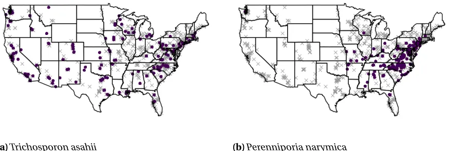
providing details about the home’s location, design features, and its occupants. Geographic and climatic information were collected based on latitude and longitude from the Climate Research Unit Time Series v3.21 Dataset (Harris et al., 2014) and the National Land Cover Database (Fry et al., 2011) for a total of over 170 covariates. From samples collected between 2012 and 2015, data was successfully sequenced for 1,331 homes spanning the 48 contiguous United States and the District of Columbia indicating the presence of 57,304 distinct fungal taxa. Of these, we focus onm=763 taxa identified in Barberán et al. (2015) as being more prevalent indoors than outdoors and on a set ofp =20 potentially influential covariates similar to those in their analysis. The presence or absence at each sampling location for two of these taxa are mapped in Figure 2.1. In the left panel,

(a)Trichosporon asahii (b)Perenniporia narymica

Figure 2.1Map of presence (purple circle) or absence (gray×) for two primarily indoor fungal taxa at each sampling location.

Trichosporon asahii, which is commonly found living on human skin, is seen to be widespread while in the right panel,Perenniporia narymicais seen to occur mainly in the mid-Atlantic region. Thus, there is evidence both that there is spatial dependence underlying the presence of fungal taxa and that the strength of that dependence varies across taxa.

2.3

Nonparametric Spatial Model

LetYj(s)be the binary indicator that OTUj=1, . . . ,mis present in the sample at spatial location

s. Suppose that we have a set ofp covariates,X(s) = [X1(s), . . . ,Xp(s)], such as those described in

Section 2.2. We assume there exists a latent continuous processZj(s)such thatYj(s) =1{Zj(s)>0}.

The latent process is modeled as

whereβj0is an intercept andβj = (βj1, . . . ,βj p)0are regression coefficients that together model

the probability that OTUj is present in a particular location. The final term,ej(s), is a multivariate

spatial process with E[ej(s)] =0 and Var[ej(s)] =1 that models dependence not captured in the

covariates between spatial locations and between OTUs. This defines a probit link for the binary responses, PYj(s) =1|X(s)

=Φ

βj0+X(s)βj

, whereΦis the standard normal cumulative density function. The assumption that Var[ej(s)] =1 is necessary because the covariate magnitudes are

identifiable only up to the ratio of effect size to variance.

Our primary goal is to develop a test to identify factors that influence microbiome composition. A covariate influences the composition if it affects the probability thatanyof the taxa will be present in a location, and thus we test the global hypotheses

H0r :βj r=0 for all j versus H1r:βj r 6=0 for somej, (2.2)

wherer and jdenote the covariate and OTU indices, respectively. The structure of this global test provides a means to identify an influential factor even if it affects only a small subset of the OTUs. It remains to describe the modeling procedure for the individual components identified in (2.1). In Section 2.3.1 we specify a Bayesian variable selection model for the regression coefficients,βj,

and in Section 2.3.2 we specify a nonparametric Bayesian model for the multivariate spatial process, ej(s).

2.3.1 Identifying influential covariates

We use a spike-and-slab prior for the coefficients,βj r, to perform variable selection (Mitchell &

Beauchamp, 1988; George & McCulloch, 1993; Kuo & Mallick, 1998). We assume that each coefficient can be written asβj r =δj rγj r for an inclusion indicator,δj r∈ {0, 1}, and magnitude,γj r ∈R. This formulation allows us to simplify the hypotheses in (2.2) in terms of the number of OTUs for which therth_{covariate is included,M}

r=

Pm

j=1δj r:

H0r:Mr=0 versus H1r:Mr>0. (2.3)

To evaluate this, we calculate the posterior probability of the null hypothesis, P(Mr=0|Y), and

compare to a thresholdt ∈[0, 1]. If the posterior probability of the null hypothesis is below the threshold, then the covariate is deemed influential.

Because we do not want to include the intercept in the variable selection process, we give it a separate priorβj0

iid

∼N(0,τ−1

0 )withτ0∼Gamma(a0,b0). Similarly, the magnitudes have the standard

conjugate formulation,γj r

indep

∼ N(0,τ−_r1)withτr

iid

∼Gamma(ar,br). The inclusion indicators are

distributedδj r

indep

∼ Bernoulli(πr), whereπr is the prior inclusion probability for the associated

The prior onπr is chosen to induce sparsity in the coefficients such that the prior probability of

the global null hypothesis in (2.3) is 0.5, reflecting no prior knowledge of whether or not a covariate is influential. In particular, the inclusion probabilities have prior density

P(πr) =ω

• ₁

B(1,θ)(1−πr)

θ−1˜_{+ (1}

−ω), (2.4)

a mixture of Beta(1,θ)and U(0, 1)distributions weighted byω∈[0, 1]and withθ ≥1. This prior has large mass on the sparse model withπr near 0, as is common in high-dimensional Bayesian

variable selection (Castillo & Vaart, 2012; Zhou et al., 2015; Roˇcková & George, 2016), but remains flexible enough to allow substantial probability for large values ofπr. Asωapproaches 1, the prior

inclusion probabilities are driven toward 0, leading to sparser coefficient vectors as in the oft used Beta(1,θ)special case, and asωdecreases to 0 the uniform component dominates and covariates will be added more readily. We can also influence the level of sparsity in the coefficients through the parameter characterizing the Beta distribution,θ. Ifθ=1 then the prior is simply U(0, 1), and the coefficient vectors will not be sparse. Asθincreases, the density associated with large values of πrdecays sharply, while density associated with small values changes less drastically, leading to a

steeper density curve. As a reasonable default, fixω=0.5 and setθ=m2_{, wheremis the number of}

taxa under consideration, which gives P(Mr=0) =0.5a priorifor each covariate, as desired.

2.3.2 Capturing residual dependence

As we show in Section 2.5, properly accounting for residual dependence is necessary for valid statis-tical inference. To model the residual dependence in (2.1), we assume thatej(s)can be decomposed

into a structural component,ξj(s), and an independent component (or nugget),εj(s), such that

e_j(s) =ξj(s) +εj(s). The structural component contributes varianceρ∈[0, 1], leaving the nugget

distributedεj(s)

iid

∼N(0, 1−ρ)to satisfy the identifiability constraint that Var[ej(s)] =1. We use a basis

expansion model forξj(s)and writeξj(s) =Ψ(s)αj, whereΨ(s) = [ψ1(s), . . . ,ψL(s)]are orthogonal

spatial basis functions common to all taxa andαj = (αj1, ...,αj L)0are their associated loadings, for

Lfinite or infinity. The model for the process now becomesej(s) =Ψ(s)αj+εj(s).

We use a Dirichlet process prior (Ferguson, 1973) for the distribution of the loadings, which can be written asαj

iid

∼f(α), wheref is the infinite mixture

f(α) =

∞

X

k=1

pk1{α=µk}. (2.5)

The mixture means have priorsµk

iid

∼ N(µ0,ρIL), whereµ0∼N(0,τ_µ−1₀IL),ρ∼U(0, 1), andτµ0 ∼

Gamma(a_µ0,b_µ0). The mixture probabilities,pk, are modeled using the stick-breaking representation

(Sethuraman, 1994) whereinp1 =V1,pk =Vk

Q

u<k(1−Vu)fork >1, andVu

iid

ensures thatpk >0 for allk and

P∞

k=1pk=1 almost surely. Rather than fix the Dirichlet process

precision parameter, we assign it an uninformative positive prior,D∼Gamma(ad,bd). With this

infinite mixture model, our prior for the distribution of the spatial random effects,ξj(s), has large

support in the class of spatial processes (Gelfand et al., 2005). In practice, the infinite mixture model in (2.5) is truncated atK terms for computational purposes. That is, we assumegk∈ {1, ...,K}for

K ≤mby settingVK =1, givingf(α) =

PK

k=1pk1{α=µk}.

The Dirichlet process prior can be viewed as a clustering model for the spatial loadings over the OTUs. If we letgj ∈ {1, 2, . . .}denote the cluster label for OTU j, then the mixture probability,pk,

can be interpreted as P(gj =k), the probability that OTU jwill be assigned to clusterk. Then, given

that OTUj has been assigned to clusterk, its associated spatial loading vector is the group mean for that cluster, i.e.,αj|gj =k isµk. In the microbiome setting, it is reasonable to believe that taxa

exhibit different spatial patterns, as in Figure 2.1, and that groups of taxa will behave similarly. For example, one may expect that organisms with similar functions or that require the same nutrients might be found in close proximity to one another. This leads to a natural expectation of clustering in the spatial effects over the OTUs.

In combination with the assumptions from the previous section, the model for the latent process becomes

Zj(s) =βj0+X(s)βj+Ψ(s)αj+εj(s)

=βj0+

p

X

r=1

Xr(s)δj rγj r+ L

X

l=1

ψl(s)αj l+εj(s),

whereβj captures the covariates’ effect on the probability that OTU jwill be present at location

s,Ψ(s)αj captures residual spatial trends, andεj(s)are independent errors. The details of the full

proposed model and its implementation, as well as a discussion of its properties, are contained in Appendix A. We also show that the covariance structure induced by our model is nonstationary in general, and that the strength of the Dirichlet process clustering controls the dependence between OTUs.

2.4

Estimating the spatial basis functions

LetS ={s1, . . . ,sn}be the set of spatial locations at which the binaryYj(s)are observed. Our

goal is to construct an estimator of the covariance of the latent process,Zj(s). To do so, we follow

the Taylor approximation technique of Hall et al. (2008). Letσ(s,s0_{)be the covariance betweenZ(s)}

andZ(s0), which fors6=s0is estimated as

ˆ σ(s,s0) =

ˆ ϑ(s,s0₎

φ{ν(ˆ s)}φ{ν(ˆ s0)}, (2.6)

whereφ(·)is the standard normal density function. This is akin to equation (10) in Hall et al. (2008), where the numerator,ϑ(s,s0), represents Cov[Y(s),Y(s0)], and the denominator acts as a scaling factor, withν(·)denoting the mean of the latent process.

However, the component estimators differ from Hall et al. (2008) because we cannot assume that the latent processes share a smooth mean process. In our setting, the mean process may differ across taxa or may be non-smooth due to its dependence on non-smooth covariates. We first obtain ˆηj(s), the predicted probability thatYj(s) =1 from separate probit regressions ofYj ontoX

for each taxon. Then we smoothm−1Pm

j=1ηˆj(·)over 2-D space using a bivariate kernel smoother

to obtain an “average” mean process ¯η(·), and let ˆν(·) =Φ−1_{{η(·)}¯ , whereΦ}−1_{(·)is the standard}

normal quantile function. In order to obtain the estimated covariance ofY(s)andY(s0), we calculate m−1Pm

j=1[Yj(s)Yj(s0)−ηˆj(s)ηˆj(s0)]and smooth these estimates using a four-dimensional kernel

smoother. The resulting smoothed estimates are collected as ˆϑ(s,s0). As is typical in nonparametric statistics, the optimal bandwidths are chosen using generalized cross-validation (Craven & Wahba, 1978; Friedman et al., 2009).

Applying this procedure to the variances will result in biased estimates (Hall et al., 2008). To remove this bias, we consider a modified estimator, ˆσ(s,s), and use the intercept of the weighted linear model

ˆ

σ(s,s0) =β0+w(s,s0)d(s,s0)β+ε,

fors6=s0and with weightsw(s,s0) =exp”−d(_ds,s₁₀0)—1(d(s,s0)≤d₁₀), whered₁₀is the distance betweens

and its 10th_{closest neighbor for some distance measured. In our application, we use the great-circle}

distance in miles.

Let ˆΣbe the initial estimate of the spatial covariance matrix with elements ˆσ(s,s0). By construc-tion, ˆΣis symmetric. However, to ensure that it is positive semidefinite, we consider its low rank approximation. Let ˜φ1(s), . . . , ˜φL(s)be the leadingLeigenvectors of ˆΣ, scaled by the square-root

of their associated eigenvalues, such that they account for a specified percentage of explained variance. In our application, we use 90%. To preserve the variance structure described in Section 2.3.2 (i.e., Var[ξj(s)] =ρ), we need to ensure that

PL

eigenvectors to obtain

ψl(s) =

– 1 PL

l=1φ˜l2(s)

™1₂ ˜ φl(s).

LetΨ= [ψ1, . . . ,ψL], whereψl ={ψl(s1), . . . ,ψl(sn)}0forl=1, . . . ,L. After this scaling process,Ψis

no longer orthogonal onRL, and thus we rotate by its right singular vectors to obtain the proposed basis functions.

Now,Ψis scaled appropriately to preserve the variance structure we require, rotated to preserve orthogonality between basis functions, and reflects the nonstationarity we expect in the data. The estimated basis functions are available only at the locations inS, and extrapolation would be required to make spatial predictions beyond thensample locations. However, our objective is not spatial prediction, but rather to account for the complex dependence structure at the sampling locations to give a valid global test of covariate effects.

Because of the reliance on generalized cross-validation to select the bandwidth parameter, the four-dimensional smoothing step to obtain the ˆϑ(s,s0)estimates can be prohibitively expensive. Two approaches to alleviating this burden are either to use a different method to select the band-width or to make the cross-validation less computationally intensive. As an example, a reasonable approach that avoids cross-validation might be to construct a variogram, identify the distance at which the correlation decays, and use that distance to set a bandwidth. Alternatively, if the data contains sampling locations that are close to one another, one could downsample the locations while approximately preserving the spatial coverage of the data. Then, generalized cross-validation can be done quickly on this smaller, representative set of locations to obtain an estimated optimal bandwidth. This latter approach is utilized in our data application in Section 2.6.

2.5

Simulation study

In this study, we consider generating data while varying the type of spatial dependence in the latent process, the existence of cross-dependence between OTUs in the latent process, the magnitude of covariate effect size, and the degree of prevalence in covariate effects, and evaluate how these factors influence the true and false positive rates of the global test in (2.3).

2.5.1 Methods

We generate data on a 15×15 grid on the unit square for a total ofn=225 spatial locations. For each ofm=50 OTUs, we draw the latent process asZj∼ Nn Xβj, 0.95Σz+0.05In

. The structure ofΣz

(Exp) Stationary dependence:Σz is populated by the exponential covariance function with

spatial range set such that the correlation between the two closest sites is 0.75, and (Nonstat) Nonstationary dependence: whereΣz(s,s0) =cos(2πs1)cos(2πs10) +sin(2πs2)sin(2πs20)for

s= (s₁,s₂).

When the setting calls for multivariate dependence in the latent process, we assume a separable covariance function and define Cov[Zj(s),Zj0(s0)] =c(j,j0)Σz(s,s0), wherec(j,j0) =0.8|j−j

0_| is the cross-dependence function. In reality, we do not expect a meaningful ordering of the OTUs, but this covariance is used to generate data with a reasonable range of cross-correlations. Thep = 20 covariates are drawn from a mean-zero Gaussian process with separable covariance function Cov[Xr(s),Xr0(s0)] =c(r,r0)Σ_x(s,s0)wherec(r,r0)is as above, andΣ_x is the exponential covariance with spatial range set such that the correlation between the two closest sites is 0.5.

Of the covariates,p0=6 are influential (i.e.,βj r is non-zero for somej) and the remainder are

unimportant for all OTUs (i.e.,βj r=0 for allj). In order to examine the ability of the algorithm to

detect covariate effects across prevalences and magnitudes, the influential covariates are split into 3 pairs. The first pair affects all OTUs, the second pair affects a randomly selected 50% of OTUs, and the final pair affects a randomly selected 10% of OTUs. Within each pair of non-zero coefficients, the first covariate is assigned a large magnitude ofβj r =0.5, and the second is assigned a small

magnitude ofβj r=−0.25. The randomization over taxa for prevalence is done independently so

that any one OTU may have 2, 4, or 6 important covariates.

Under each of the simulation settings we generateN =50 replicate datasets and fit the proposed spatial nonparametric model and several competing models:

(PERM) PERMANOVA (Anderson, 2001; McArdle & Anderson, 2001), a permutation-based hypoth-esis test as implemented in the

R

vegan 2.4-3

(Mat) Parametric spatial model whereej = [ej(s1), . . . ,ej(sn)]0from (2.1) is modeled using a

Mat´ern covariance function. The smoothness has priorκ∼U(0, 2)(Stein, 1999; Banerjee, 2005), and the range has prior log(ζ)∼N(0,σ_ζ2)whereσ2_ζis set such that the 99th_percentile

of the prior distribution for the range is the maximum observed distance.

(SNP) Proposed nonparametric spatial model using the nonstationary basis detailed in Section 2.4, with the maximum number of groups set toK =m.

setting. Our focus is on identifying covariates that are borderline cases, i.e., factors that influence only a few taxa. The sharper cut of this simplified prior near the origin makes the sampler less likely to include these covariate spuriously. To determine sensitivity to this prior specification, we also ran the simulation using the mixture prior in (2.4) with the recommended default values. The results are qualitatively the same, with improved performance for Mat in identifying small magnitude covariates but a reduced ability to identify low prevalence covariates. The model performance for SNP is broadly unchanged. The remainder of the prior specifications are detailed in Appendix A.2. The models are run for a total of 40,000 iterations with a burn-in period of 10,000, and the posterior samples are thinned by 2. We deem therth_{covariate to be influential if the associated posterior}

probability of the null is below 0.05, i.e., P(Mr=0|Y)<0.05, for the Bayesian models, or if its P-value

from PERMANOVA is below 0.05.

For each dataset, we evaluate the models using true positive rate (TPR) and false positive rate (FPR), presented in Table 2.1. LetM_r∗be the indicator that therthcovariate is truly influential. The true positive rate is the percent of truly influential covariates correctly classified as influential by the model for a given thresholdt,

TPR(t) =

p

P

r=1

M_r∗1{P(Mr=0|Y)<t}

p0

.

The false positive rate is the percent of truly unimportant covariates that are incorrectly classified by the model as influential,

FPR(t) =

p

P

r=1

(1−M_r∗)1{P(Mr=0|Y)<t}

p−p₀ .

We also consider a “registered” true positive rate, where the threshold for each method is set to control its false positive rate at or below 0.05. In other words, for each model and simulated data set, we find the largest thresholdT such that FPR(T)≤0.05, and use this calibrated threshold to evaluate the model. In the case of PERMANOVA, the posterior probability of the null is replaced by the P-value. This allows us to compare the power of the methods on an even footing in Table 2.2. Finally, in Table 2.3, we consider the inclusion rate for the influential covariates for each model, broken out by magnitude of the covariate effect, small (S) or large (L), and the prevalence of the covariate effect, 100%, 50%, or 10%. The inclusion rate (IR) is defined as the proportion of theN simulation runs for which the method correctly classified the covariate as influential,

IR(t) = 1 N

N

X

s=1

1{P Ms,r∗=0|Y

for each of ther∗=1, . . . ,p0influential covariates. As in the global results presented in Table 2.1, we

use a fixed threshold oft =0.05.

2.5.2 Results

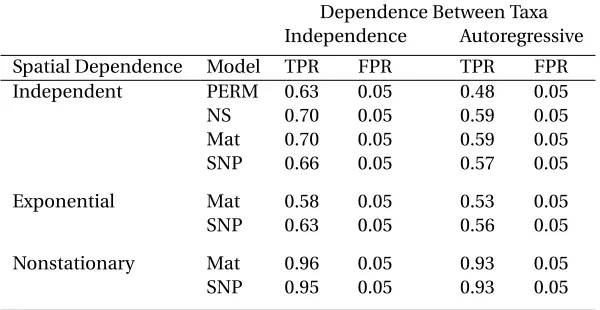
Table 2.1Summary of true positive rate (TPR), false positive rate (FPR), and average model fitting time in minutes for PERMANOVA (PERM), the nonspatial (NS), parametric Mat´ern (Mat), and proposed nonpara-metric (SNP) models.

Dependence Between Taxa Independence Autoregressive Spatial Dependence Model TPR FPR Time TPR FPR Time Independence PERM 0.62 0.05 3.75 0.49 0.06 3.68

NS 0.38 0.00 21.59 0.38 0.01 21.58 Mat 0.40 0.00 426.09 0.39 0.01 418.41 SNP 0.37 0.00 34.90 0.38 0.00 35.05

Exponential PERM 0.96 0.80 3.98 0.87 0.61 3.75 NS 0.86 0.48 22.18 0.81 0.43 21.73 Mat 0.54 0.04 232.48 0.51 0.04 228.38 SNP 0.71 0.10 36.82 0.67 0.10 35.61

Nonstationary PERM 0.81 0.49 3.74 0.81 0.49 3.88 NS 0.91 0.43 24.01 0.90 0.47 25.27 Mat 0.85 0.00 231.90 0.84 0.01 237.80 SNP 0.93 0.02 39.36 0.94 0.05 40.51

As is evident in Table 2.1, in the case of no spatial dependence in the data, PERM outperforms the Bayesian models. The Bayesian tests are more conservative, but after tuning the FPR to be 0.05 (Table 2.2), they have comparable or increased true positive rates as compared to PERMANOVA. The false positive rate for PERM is well-controlled even in the face of multivariate dependence, which is reasonable given that the permutation is done at the sampling location level and thus the structure of any cross-dependence between taxa is preserved.

However, in the presence of spatial dependence, PERMANOVA fails to preserve the size of the hypothesis test and has false positive rates an order of magnitude higher than expected. This is perhaps not unexpected as the pseudo-F test is built on the assumption of exchangeability across sampling locations. Blind application of these permutation-based methods in settings where spatial independence across sampling locations is not a reasonable assumption will result in misleading conclusions.

Table 2.2Summary of “registered” true positive rate (TPR) and false positive rate (FPR) for PERMANOVA (PERM), the nonspatial (NS), parametric Mat´ern (Mat), and proposed nonparametric (SNP) models. If values are not provided, there is no threshold value or significance level that controls the false positive rate at the required level.

Dependence Between Taxa Independence Autoregressive Spatial Dependence Model TPR FPR TPR FPR Independent PERM 0.63 0.05 0.48 0.05 NS 0.70 0.05 0.59 0.05 Mat 0.70 0.05 0.59 0.05 SNP 0.66 0.05 0.57 0.05

Exponential Mat 0.58 0.05 0.53 0.05 SNP 0.63 0.05 0.56 0.05

Nonstationary Mat 0.96 0.05 0.93 0.05 SNP 0.95 0.05 0.93 0.05

discriminating between important and unimportant factors. Therefore, we exclude these mod-els in Table 2.3, where we present the inclusion rate for the influential covariates broken out by prevalence and magnitude for each of the models. As before, in the case of spatial independence, PERM outperforms the Bayesian models, which all perform similarly. However in the case of spatial dependence, breaking out the model performance in this way allows us to see the contrast between the Bayesian spatial models. In particular, we can see that SNP outperforms the parametric model in identifying covariates with low prevalence and/or small magnitudes, which is our primary focus. Under the exponential covariance structure, SNP picks up the low prevalence, small magnitude covariate 16-20% of the time, whereas the parametric model selects it in only 0-4% of the replications. Similarly, under the nonstationary covariance structure, the parametric model selects the covariate in only 20-28% of replications, as opposed to the 60-66% of replications for SNP.

Table 2.3Inclusion rate for influential covariates for PERMANOVA (PERM), the nonspatial (NS), para-metric Mat´ern (Mat), and proposed nonparapara-metric (SNP) models, broken out by covariate magnitude (S=Small, L=Large) and prevalence (100%, 50%, 10%).

Dependence Covariate Prevalence and Magnitude Spatial Between Taxa Model 100% L 100% S 50% L 50% S 10% L 10% S Ind Ind PERM 1.00 0.38 1.00 0.62 0.60 0.14

NS 1.00 0.16 0.84 0.02 0.28 0.00 Mat 1.00 0.18 0.86 0.02 0.32 0.00 SNP 1.00 0.06 0.78 0.02 0.34 0.00 AR(0.8) PERM 0.92 0.26 0.98 0.26 0.42 0.12 NS 1.00 0.14 0.76 0.08 0.32 0.00 Mat 1.00 0.14 0.76 0.08 0.36 0.00 SNP 1.00 0.10 0.78 0.06 0.34 0.00

Exp Ind Mat 1.00 0.46 0.94 0.22 0.62 0.00 SNP 1.00 0.76 0.96 0.56 0.76 0.20 AR(0.8) Mat 1.00 0.38 0.94 0.18 0.50 0.04 SNP 1.00 0.64 1.00 0.48 0.74 0.16

Nonstat Ind Mat 1.00 1.00 1.00 0.92 0.92 0.28 SNP 1.00 1.00 1.00 1.00 0.98 0.60 AR(0.8) Mat 1.00 1.00 1.00 0.88 0.94 0.20 SNP 1.00 1.00 1.00 0.96 1.00 0.66

2.6

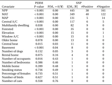
Data Analysis

In light of PERMANOVA’s demonstrated failure to preserve the size of the hypothesis test in the face of spatial and multivariate dependence, we revisit the analysis of Barberán et al. (2015) in which the authors determined which, if any, of a set of environmental and household covariates affect the indoor fungal community composition of homes. The covariates of interest included mean annual precipitation (MAP), mean annual temperature (MAT), net primary productivity (NPP), elevation, age of the home, number of bedrooms, number of inhabitants, female-to-male ratio of the home’s inhabitants, smoking status, number of dogs/cats/birds, whether or not the home has a basement, and number of days with the windows open. Using PERMANOVA, they find that the effects of outdoor variables and geographic location are more pronounced than the household covariates, but note that the presence of a basement in the home, the age of the home, and the presence of a dog also affect the composition of the indoor fungal microbiome.

(central air-conditioning, central heat, window air-conditioning). NPP was missing for 81 of the sampling locations, and when considering only indoor fungal taxa, an additional 24 sampling locations had no present taxa. These locations have been removed, leavingn=1,226 locations and p=20 covariates in the analysis.

Using both PERMANOVA and the proposed nonparametric method, we investigated each covari-ate’s ability to affect the composition of the taxa identified as the indoor fungal microbiome. SNP was run for 80,000 total iterations, keeping the final 30,000 posterior samples. Unlike in the simulation study, the maximum number of groups is set toK =500<m. We utilized the downsampling strategy discussed in Section 2.4 to build the spatial basis functions. The first few estimated basis functions are mapped in Figure 2.2. The first several functions reflect the nonstationarity in the data, while

Figure 2.2Maps of the first four spatial basis functions estimated from the WLOH data.

number of taxa for which the covariate is selected, and a count of the number of taxa for which the associated coefficient value is positive or negative, assessed asP763_j=11{P(βj r >0|Y)>0.975}and

P763

j=11{P(βj r<0|Y)>0.975}, respectively, for the proposed model.

Table 2.4Summary of variable selection results from PERMANOVA (PERM) and the proposed spatial nonparametric method (SNP). P-values are reported from PERM, and the posterior probability of the null hypothesis, the expected number of taxa for which the covariate is included, and the number of taxa for which the coefficient value is positive or negative are reported for SNP.

PERM SNP

Covariate P-value P(Mr=0|Y) E[Mr|Y] #Positive #Negative NPP <0.001 0.00 445 38 161 MAT <0.001 0.00 349 40 122 MAP <0.001 0.00 131 5 14 Central A/C <0.001 0.00 117 6 5 Multifamily dwelling 0.038 0.00 82 9 0 Forested <0.001 0.00 35 0 0 Elevation <0.001 0.00 15 0 1 Window A/C <0.001 0.00 15 0 1 Older home 0.078 0.00 13 0 0 Central heat 0.015 0.03 11 0 0 Basement <0.001 0.04 8 0 0 Number of dogs 0.152 0.05 5 0 0 Rental home 0.075 0.16 4 0 0 Number of occupants 0.016 0.43 1 0 0 Number of bedrooms 0.386 0.46 1 0 0 Mobile home 0.289 0.48 1 0 0 Smoking status 0.756 0.49 1 0 0 Percentage of females 0.735 0.51 1 0 0 Number of birds 0.627 0.51 1 0 0 Number of cats 0.558 0.76 0 0 0

geographic and climatic factors are most influential to the indoor fungal microbiome composition. The household covariates that appear as influential are whether or not the home is older, the presence of a basement, whether or not the home is a multifamily dwelling, and whether or not the home has air-conditioning or central heating, all of which play a role in increasing the interaction between the indoor environment and the outdoors.

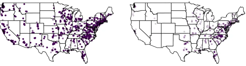
The 763 species are grouped into an estimated (posterior mean) 47 clusters. The largest clusters, based off of ak-means clustering algorithm with 47 clusters and using 1−P(gj =gj0)as the dissim-ilarity matrix, contain taxa that exhibit little spatial clustering and tend to be present across the country. The smaller clusters tend to group together taxa that exhibit more localized presence. For example, in Figure 2.3, the left panel displays the presence for the 100 taxa assigned to the largest cluster and the right panel displays the presence for the 3 taxa assigned to a smaller cluster.

Figure 2.3Map of presence for taxa assigned to a large cluster of 100 taxa and a small cluster of 3 taxa. A darker point indicates that a higher number of taxa are present in a location.

In as much as our results add to those of previous analyses using data from the WLOH project, it is worth commenting about the additional biological insights our approach offers. Barberán et al. (2015) found that, compared to bacteria, the composition of fungi in homes tended to be much more strongly driven by outdoor environmental conditions. In our analysis, this conclusion is even more strongly supported. The primary factors associated with differences in the composition of indoor fungi among households were those associated with climate and its effects, and nearly all (94.8%) significant associations of individual taxa with particular covariates were associations with these environmental factors.

including multiple taxa of the speciesXylobolus annosus. Conversely, species that became less common under high NPP tended to be from the generaAlternaria,Cladosporum,Aspergillus, and Phoma, many of which are associated with decaying plant material. Fungi from decaying plant material, much of which is in leaf litter, might be more likely to become airborne in open habitats such as grasslands. Many species were also influenced by the direct effects of the mean annual temperature or precipitation in the region in which a house was located.

One of the few non-environmental covariates identified as influential was whether or not the home is a multifamily dwelling. Multifamily dwellings tended to favor fungi associated with hu-man bodies or foods. These included threeCandidataxa,Cryptococcus oeirensis,Penicillium concetricum, and the brewer’s yeast (Saccharomyces cerevisae). Also more common in these homes wereRhodotorula mucilagnosaandCystofilobasidium capitatum, both of which do well under stressful conditions, such as those associated with bathrooms that are frequently cleaned. The way in which a house was heated or cooled also influenced which species were present. In particular, as has been noted in smaller scale studies (Hamada & Fujita, 2002), we confirm here that houses with air conditioning tend to be more likely to haveCladosporiumandPenicilliumfungi, which are known to grow in air conditioning units and then spread through houses. Air conditioners were also associated with several other fungal species, including the wood rot fungusPhysisporinus vitreus, a pattern for which the mechanistic links deserve more study.

Considering that the homes we studied differed greatly in their size, number of occupants, age, design, and much more, the fact that these variables influence so very little of fungal composition is striking. Houses, in general, favor some fungi relative to others and yet just which species appears to depend nearly exclusively on where the house is built.

2.7

Discussion

In this paper, we introduced a nonparametric Bayesian model for identifying factors that influence microbiome composition, as well as a covariance estimator amenable to high-dimensional, binary data akin to that of Hall et al. (2008). The proposed model uses spike-and-slab variable selection to identify covariates that influence the occupancy probability of even a small subset of the taxa. It also utilizes a set of orthogonal, data-driven spatial basis functions and a Dirichlet process prior over their associated loadings to cluster the OTUs into groups of taxa that exhibit similar spatial responses, allowing dimension reduction in both the number of spatial locations and the number of taxa under consideration, greatly alleviating the computational burden compared to a parametric spatial model.

not well-controlled. We also showed that the proposed model is able to better identify low prevalence and/or small magnitude covariate effects as compared to a parametric spatial competitor.

We applied our proposed model to the indoor fungal microbiome from the Wild Life of Our Homes project as identified in Barberán et al. (2015). We were able to broadly substantiate their conclusion that geography and climate are the most influential factors affecting indoor fungal communities, and we provided additional detail in describing how factors affect particular taxa rather than simply classifying factors are influential or unimportant.

CHAPTER

3

BAYESIAN VARIABLE SELECTION FOR

HIGH-DIMENSIONAL RANK DATA

3.1

Introduction

The advancement of high throughput sequencing technologies made previously cost-prohibitive study of DNA material accessible in a variety of fields. In particular, interest in studying microbiomes, which are communities of microorganisms that occupy a specific ecological niche, has surged. To date, much of the work in the microbiome arena has focused on drawing connections and describing correlations between microbial community composition and specific outcomes. For example, childhood exposure to low fungal diversity has been linked to development of asthma (Dannemiller et al., 2014), imbalances in microbiome composition have been linked to Type 2 diabetes (Qin et al., 2012), and reduced diversity in the gut microbiome has been tied to obesity (Ley et al., 2005; Turnbaugh et al., 2009) and Crohn’s disease (Dicksved et al., 2008). Recently, there has been an effort to begin identifying characteristics of “healthy” microbiomes within the body (Clemente et al., 2012; Human Microbiome Project Consortium, 2012), but fully leveraging this information requires knowledge of how to address complications in addition to identifying them. However, the availability of statistical tools to determine the effect of external factors on the composition of these communities is limited.

complex dependence, and non-normality. The raw abundance counts frequently display zero-inflation and overdispersion, and as an artifact of the sequencing process the counts reflectrelative information rather than absolute information because the total amount of DNA material in a partic-ular sample varies. Thus, standard multivariate statistical approaches are not applicable.

To overcome these complications, analyses frequently reduce the multivariate (or community) response to a summary metric (e.g., species richness, Shannon diversity index) or a measure of dissimilarity between samples, such as Euclidean or Bray-Curtis dissimilarity (Bray & Curtis, 1957). One of the most popular tools for analyzing communities takes the latter approach. “PERmutational Multivariate ANalysis Of VAriance” (PERMANOVA; Anderson, 2001; McArdle & Anderson, 2001) uses a nonparametric permutation-based test to determine which covariates affect dissimilarity between samples. These tools are applicable to many types of response variables (e.g., counts, presence-absence), but they can be difficult to interpret. These tests partition the pairwise dissimilarity between samples with respect to covariates, but do not provide clarity onhowa covariate affects the composition or which taxa may be affected.

Recently, tools have been developed to analyze the compositional counts to address some of these concerns. Some propose transformations of the relative proportions, which are then treated using standard multivariate statistical methods (Aitchison, 1986; Fernandes et al., 2013; Mandal et al., 2015). A variety of methods have assumed a parametric model for the abundance counts, including the Dirichlet-multinomial (Chen & Li, 2013; Wadsworth et al., 2017), the negative binomial (Zhang et al., 2017), or the logistic normal multinomial (Xia et al., 2013; Grantham et al., 2017), among others. Still others have suggested nonparametric approaches, utilizing generalized linear models (Warton, 2011) or regression kernels (Zhao et al., 2015).

a variety of sources (Johnson et al., 2002; Deng et al., 2014), and to combine rank data with other data types (Barney et al., 2015).

In this work, we develop a procedure that identifies covariates that influence microbiome composition, as quantified by taxa rankings, using a hierarchical Bayesian approach. We utilize a multivariate order statistics model for the ranks and a spike-and-slab prior for variable selection. In an extension to the base model, we detail the addition of a flexible basis function model to capture cross-dependence between taxa. This model provides global hypothesis tests of whether or not a covariate influences microbiome composition that can be used to screen many potential covariates, allowing the identification of targets for intervention or further research. Additionally, the model provides for local hypothesis tests for individual taxa which allows for a richer characterization of the mechanism through which external factors can affect microbial communities.

The remainder of the paper is laid out as follows: in Section 3.2, we introduce the motivating data from The American Gut Project; in Section 3.3, we describe the modeling procedure; in Section 3.4, we present a simulation study demonstrating the efficacy of our procedure against several competing models; in Section 3.5, we present an application of our method to a healthy subset of The American Gut Project; and we conclude with a brief summary and discussion in Section 3.6.

3.2

Motivating Data

The American Gut Project (americangut.org) is a citizen-science project with the twin goals of allowing participants to learn about their own microbes and arming researchers with publicly accessible data to study the relationships between microbes and human health. Participants in the project receive a sampling kit and instructions detailing the locations from which to take samples and how to handle samples safely. In addition to providing samples, participants are asked to fill out a survey with diet and lifestyle questions. After the samples are returned, the DNA is amplified using the direct PCR approach, sequenced, and classified into Operational Taxonomic Units (OTUs).

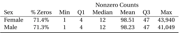
We focus on a subset of the data identified by The American Gut Project as the “healthy subset”. These stool samples are from 3,942 adult participants of healthy weight, with no antibiotic use in the previous year, and no history of inflammatory bowel disease or diabetes. We stratify the data by sex, resulting in the removal of 88 participants without a female or male designation and an additional 31 participants with incomplete covariate information. Further, we include only OTUs that are present in at least 10% of the samples in our analysis. The final data include abundance counts form=416 taxa inn=3,823 samples representing 2,019 female subjects and 1,804 males. A summary of the counts by sex are given in Table 3.1.

Table 3.1Summary of the abundance counts in a subset of the American Gut Project by sex.

Nonzero Counts

Sex % Zeros Min Q1 Median Mean Q3 Max Female 71.4% 1 4 12 98.51 47 43,940 Male 71.3% 1 4 12 98.23 47 41,049

changes can affect the gut microbiome, though the relationship is complicated (Santacruz et al., 2009; Queipo-Ortuño et al., 2013; Kang et al., 2014). As such, we considerp=21 covariates, which are selected to reflect dietary differences between subjects, exercise habits, and lifestyle. We include indicators for broad dietary habits: whether or not a subject is gluten-free and whether or not a subject takes a multivitamin or probiotic. In addition, we consider more specific habits: whether or not a subject “regularly” (as opposed to “rarely” or “never”) consumes fruit, dairy, poultry, red meat, seafood, vegetables, or whole grains and whether or not a subject consumes animal products treated with antibiotics, alcohol, or artificial sweeteners. There are also indicators for physical activity: whether or not a subject exercises regularly (at least 3-5 times per week) and whether or not they have gained or lost more than 10 pounds in the past year. We also include age in years, BMI, the presence of a cat in the home, the presence of a dog in the home, and whether or not the subject regularly uses cosmetics. The goal of this analysis is to identify which, if any, of these covariates influences microbiome composition for female or male subjects.

3.3

Model

LetCi j∈ {0, 1, 2, . . .}be the read count of OTUj=1, . . . ,min samplei=1, . . . ,n. Rather than model

the counts directly, we retain only the indices and ranks of the nonzero counts, denoted byYi j. As is

commonly argued in robust statistics, this transformation is insensitive to extreme counts such as those in Table 3.1. In particular, ifCi j =0 then we setYi j=0, and ifCi j is thekthlargest nonzero

count in samplei then we setYi j =k. In the examples we consider, ties between nonzero counts

are rare and so we simply randomize the order of theYi j to break ties. Ties could be handled more

thoroughly within our framework by using slightly more elaborate orderings of the latent variables. We adopt a multivariate order statistics model (Yao & Böckenholt, 1999; Yu, 2000) wherein the discrete data,Yi j, are related to latent continuous random variables,Zi j. We assume that ifYi j=0

thenZ_{i j}<0 and if 0<Y_{i j} <Y_{i j}0then 0<Z_{i j} <Z_{i j}0. We then assume that the latent variables depend linearly on covariatesXi= (Xi1, . . . ,Xi p), which have been centered and scaled, and write

Zi j =βj0+Xiβj+ei j, (3.1)