CHO, EUN HEA. Computation for Markov Chains. (Under the direction of Prof. Carl D. Meyer).
A finite, homogeneous, irreducible Markov chain C with transition probability matrix P possesses a unique stationary distribution vector πT. The questions one can pose in the area of computation of Markov chains include the following:
• How does one compute the stationary distributions? • How accurate is the resulting answer?
In this thesis, we try to provide answers to these questions.
by
Eun Hea Cho
a dissertation submitted to the graduate faculty of
north carolina state university
in partial fulfillment of the
requirements for the degree of
doctor of philosophy
department of mathematics
applied mathematics
raleigh
2000
approved by:
Grace Eun-Hea Cho graduated from Yonsei University in Seoul, Korea with a BS de-gree in Mathematics. She continued her studies at Universit¨at Hamburg in Germany and received the Diplom Mathematik/Informatik under the direction of Prof.Helmut Strade. After working as a software engineer at dvg-Datenverarbeitungsgesellschaft mbH in Hannover, Germany, she came to North Carolina State University to pursue a doctoral degree in Applied Mathematics.
First of all, I would like to express my gratitude to my advisor and teacher, Dr. Carl D. Meyer, for teaching me and guiding me for the past five years. I am thankful for his enthusiasm, encouragement, and patience through this work and also for his advice on my research and my career.
Furthermore, I want to thank Dr. John Bishir, Dr. Billy Stewart, and Dr. Ernie Stitzinger for serving on my advisory committee. I also thank the members of the Graduate Student Seminar in Numerical Analysis for the valuable experience they provided. Many thanks go to the staff of our department - Mary Byrd, Janet Early, Dianne Hartgrove, April Jackson, and especially, Brenda Smith - for helping me whenever I needed.
Finally, I would like to thank Jamey for standing by me for the past five years and also proof-reading this dissertation.
List of Tables vii
1 Introduction 1
2 Background 3
2.1 Notations . . . 3
2.2 M-Matrices . . . 5
2.2.1 M-Matrices . . . 5
2.2.2 M-Matrices with property c . . . 7
2.3 Nonnegative Matrices . . . 8
2.3.1 Positive Matrices and Perron Theory . . . 8
2.3.2 Nonnegative Matrices and Perron-Frobenius Theory . . . 10
2.4 Properties of Markov Chains . . . 13
2.4.1 Markov chains and Stochastic Matrices . . . 14
2.4.2 Limiting Properties of Transition Probability Matrices . . . . 15
2.5 Computation of Stationary Distribution . . . 17
2.5.1 Gauss Elimination . . . 18
2.5.2 Gauss Elimination and Markov Chains . . . 19
2.6 Ergodic Coefficients . . . 26
2.6.1 Definition of Ergodic Coefficients . . . 27
2.6.2 Generalization of Ergodic Coefficients . . . 28
2.6.3 Explicit Forms for Ergodic Coefficients . . . 31
2.6.4 More Properties of Ergodic Coefficients . . . 33
2.6.5 Weak and Strong Ergodicity . . . 35
3 Perturbation Theory of Finite Irreducible Markov Chains 38 3.1 Sensitivity and Group Inverse . . . 40
3.1.1 Group Inverse and Limiting Properties . . . 40
3.1.2 Perturbation Bounds in Terms of Group Inverse . . . 43
3.2.2 Perturbation Bounds in Terms of Ergodic Coefficients . . . 52
3.3 Sensitivity and Eigenvalues . . . 55
3.3.1 Eigenvalues of P, Z, A, A# and Their Ergodic Coefficients . . . 55
3.4 Sensitivity of a Markov Chain and Mean First Passage Times . . . 56
3.4.1 Mean First Passage Times . . . 57
3.4.2 Perturbation Bounds in Terms of Mean First Passage Times . . . 58
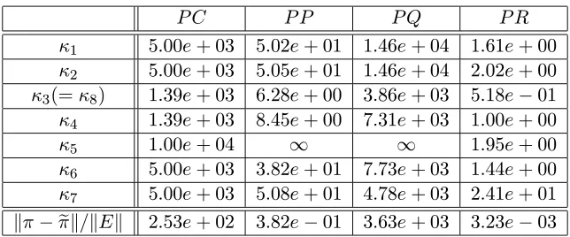
3.5 Comparison of Condition Numbers and Numerical Results . . . 60
3.5.1 Absolute Component-Wise Bounds . . . 60
3.5.2 Relative Component-Wise Bounds . . . 61
3.5.3 Norm-Wise Bounds . . . 61
3.5.4 Comparison of Condition Numbers . . . 62
3.5.5 An Open Question and Observations . . . 68
4 Nearly Uncoupled Markov Chains 73 4.1 Definitions and Properties . . . 74
4.1.1 Nearly Uncoupled Markov Chains . . . 74
4.1.2 Stochastic Complements . . . 75
4.1.3 Coupling Matrix . . . 79
4.1.4 Exact Aggregation/Disaggregation Method . . . 80
4.2 Approximation to Stationary Distribution of NUMC . . . 81
4.2.1 Dropping Method -Simplest Approximation to Stochastic Complements . . . 83
4.2.2 Inverse Approximation Method -Approximation to Stochastic Complements . . . 84
4.2.3 Hybrid Method . . . 85
4.2.4 Dynamic Reaggregation . . . 87
4.2.5 Marginal Distribution Method -Approximation to Censored Distribution . . . 89
4.2.6 Nonstochastic Method -Approximation to Stationary Distribution of NUMC . . . 90
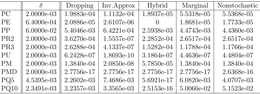
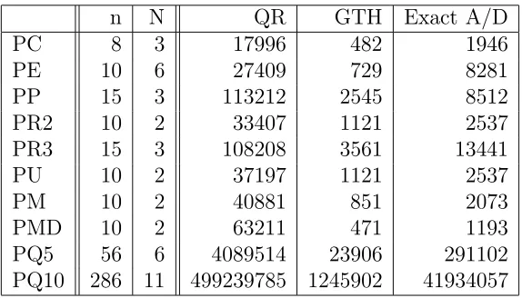
4.2.7 Numerical Experiments . . . 94
4.3 Errors in Approximation . . . 107
4.3.1 Bound for Stewart’s Nonstochastic Method . . . 108
4.3.3 Error Bounds . . . 113 4.3.4 Interpretation of Error Bound and Observations . . . 121
5 Summary 123
A Useful Lemmata 125
List of References 131
3.1 Condition Numbers . . . 68
4.1 Accuracy of Approximations . . . 105
4.2 Effectiveness (flops): Inexact A/D . . . 106
4.3 Effectiveness (flops): Other Methods . . . 106
Introduction
A finite, homogeneous, irreducible Markov chainC with transition probability matrix P possesses a unique stationary distribution vector πT. In other words, there is a unique vector π such that
πTP =πT, π >0, πTe= 1,
where e is the column vector of all ones. The questions one can pose in the area of computation of Markov chains include the following:
• How does one compute the stationary distributions? • How accurate is the resulting answer?
In this thesis, we try to provide answers to these questions.
The thesis is divided in two parts. The first part deals with the perturbation theory of finite, homogeneous, irreducible Markov Chains, which is related to the first question above. The purpose of this part is to analyze the sensitivity of the stationary distribution vector πT to perturbations in the transition probability matrix P. The second part gives answers to the question of computing the stationary distributions
of nearly uncoupled Markov chains (NUMC).
The thesis is organized as follows. In the next chapter, we clarify the notations used throughout the thesis and provide background materials relevant to the theory of Markov chains. Included are M-matrices, nonnegative matrices, limiting proper-ties of Markov chains, Gauss elimination and Markov chains, and an introduction
Background
This chapter contains background materials for the theory of Markov chains. After a brief summary of notations, we review the theory of M-matrices and nonnegative matrices. In § 2.4, basic terminologies and limiting properties of Markov chains are summarized. The problems using Gauss elimination for computing the stationary distribution of a Markov chain are discussed in § 2.5, as well as a variant of Gauss elimination proposed by Grassmann, Taskar, and Heyman. The last section is a brief introduction of ergodic coefficients which play a main role in the perturbation theory of Markov chains.
2.1
Notations
Although notations are declared in each section or in each theorem, we explain here the following notations used often throughout the thesis.
• R: the field of real numbers • C: the field of complex numbers
• Rn: the set of column vectors of length n whose entries belong toR • Cn: the set of column vectors of length nwhose entries belong to C • I: the identity matrix of appropriate size
• e: the column vector of all ones of appropriate size
• ek: the k-th column of the identity matrix of appropriate size • 0: the vector or matrix of all zeroes of appropriate size • C: a Markov chain
• P: the transition probability matrix of a given Markov chain • P∞: the limiting matrix of P
• πT: the stationary distribution vector of a given Markov chain • Z: the fundamental matrix of a Markov chain
• A#: the group inverse of a matrix A
• τk·k(A): the ergodic coefficient of a matrixA with equal row sums with respect to a given norm k · k
• aij: the (i, j) component of a matrix A • Ai∗: the ith row of a matrix A
• A∗j: the jth column of a matrix A
• A(j): the principal submatrix of a matrix A obtained by
deleting the j-th row and column from A. • N(A): the null space of a matrix A
• R(A): the range of a matrixA • rank (A): the rank of a matrix A
• k · kp: the p-norm of a vector or of a matrix (1≤p≤ ∞)
The 1-norm of a vector is the sum of the absolute values of the component.
The ∞-norm of a vector is the largest absolute value among the components.
2.2
M-Matrices
In this section, we review the definition and properties of an M-matrix, which are cited and used in various parts of the thesis. Most of the material in this chapter is taken from Nonnegative Matrices in the Mathematical Sciences by Berman and Plemmons[2, Chapter 6].
2.2.1
M-Matrices
For a square matrix A of order n, denote the spectrum by σ(A) and the spectral radius by ρ(A).
Definition 2.2.1.1
(a) A square matrixA with nonpositive off-diagonal elements is called a Z-matrix. Denote the set of n×nZ-matrix by Zn×n:
Zn×n≡ {A= (aij)∈Rn×n : aij ≤0 fori6=j}.
(b) An M-matrix A is a square matrix which can be written in the form
A=sI−B with s≥ρ(B), B≥0.
Any square matrix A has the form A =sI −B with s > 0, B ≥0 if and only if it has nonpositive off-diagonal and nonnegative diagonal entries:
A=
a11 −a12 −a13 . . . −a1n −a21 a22 −a23 . . . −a2n
..
. ... . .. ...
..
. ... . .. ...
−an1 −an2 −an3 . . . ann ,
where aij ≥0, for alli, j = 1,2,· · ·, n.
which we then use for the rest of the thesis. For a complete list, see Berman and Plemmons[2, Chapter 6].
Theorem 2.2.1.1 Let A be a Z-matrix. Then the following are equivalent:
(1) A is an M-matrix.
(2) The real part of each nonzero eigenvalue of A is positive.
(3) A is nonnegative stable, i.e., every eigenvalue of A has a nonnegative real part.
(4) All of the principal matrices of A are nonnegative.
(5) Every real eigenvalue of each principal submatrix of A is nonnegative.
(6) A+D is nonsingular for all positive diagonal matrices D. (7) A+αI is nonsingular for all α >0.
Theorem 2.2.1.2 Let A be a Z-matrix. Then the following are equivalent: (1) A is a nonsingular M-matrix.
(2) Every real eigenvalue of A is positive.
(3) A is positive stable, i.e., every eigenvalue of A has a positive real part. (4) All of the principal matrices of A are positive.
(5) Every real eigenvalue of each principal submatrix of A is positive.
(6) A+αI is nonsingular for all α≥0.
(7) A issemi-positive, i.e., there exists a positive vectorx >0 such that Ax >0. (8) There is a nonnegative vector x≥0 (6= 0) such that Ax >0.
(9) A is inverse-positive, i.e., A is nonsingular and its inverse is nonnegative:
2.2.2
M-Matrices with property c
In this section, a special class of M-matrices is considered and the definition and properties relevant to the thesis are listed. We start with general limiting properties of a square matrix.
Definition 2.2.2.1 Let T be a square matrix. (a) T is said to be convergent if P∞k=0Tk exists.
(b) T is said to be semi-convergent if limk→∞Tk exists.
Lemma 2.2.2.1 Let T be a square matrix. For an eigenvalue λ of T, let Ind(λ)
denote the index ofλ. (The index of an eigenvalue λ is the size of the largest Jordan
block associated with λ.)
(a) T is convergent if and only if ρ(T)<1.
(b) T is semi-convergent if and only if each of the following holds:
(i) ρ(T)≤1, and
(ii) if ρ(T) = 1, then 1 is an eigenvalue of T with Ind(1) = 1, and 1 is the only eigenvalue of T on the spectral circle.
Definition 2.2.2.2 An M-matrix Ais said to haveproperty c if it can be split into
A=sI−B, with s≥ρ(B), B ≥0, where T ≡B/s is semi-convergent.
Lemma 2.2.2.2 An M-matrix A has property c if and only if Ind(A)≤1.
(Ind(A) of a matrix A is defined to be Ind(0) if A is singular, and zero, otheriwse.) Lemma 2.2.2.3 Let A be a Z-matrix. If there exists x > 0 such that Ax≥ 0, then
A is an M-matrix with property c.
(a) rank(A) =n−1.
(b) There is a positive vector x >0 such that Ax≥0. (c) A has property c.
(d) Each principal submatrix of A other than A itself is a nonsingular M-matrix.
(e) A is almost monotone, i.e., if Ax≥0, then Ax= 0.
2.3
Nonnegative Matrices
The transition matrix of a Markov chain is a (row) stochastic matrix, i.e., it is a square nonnegative matrix with row sums equal to 1. Many of the properties of stochastic matrices are from the general theory of nonnegative matrices. In this section, Perron theory for positive matrices and Frobenius theory for nonnegative matrices are reviewed. Detailed study of this subject is to be found in Berman and Plemmons[2] and Seneta[47]. This section is a summary of relevant material for this thesis, taken from these two books and from the lecture notes in Theory of Matrices and Applications by Meyer at North Carolina State University [37].
2.3.1
Positive Matrices and Perron Theory
A square matrix A= (aij) of order nis said to be positive if all of its elements are positive: aij >0, for alli, j = 1,2,· · ·, n. In this case, we write
A >0.
The notation of >(<) and ≥(≤) for matrices is often used in a different way in the theory of definite matrices. Therefore before we continue, we will clarify the notation to be used here.
A6=B if there is at least one element aij such thataij 6=bij. The same definitions of > and ≥ apply for vectors as well. Moreover, to denote the matrix of the entrywise absolute value, we us the following notation
|A| ≡(|aij|).
For a vector x, the notation |x| is defined accordingly.
The influence of positivity of a matrix on its eigenstructure was intensively studied by Perron[40], and the following theorem summarizes that theory.
Theorem 2.3.1.1 (Perron Theory[40])
Let A be a positive matrix of order n. Denote the spectrum and the spectral radius of
A by σ(A) and ρ(A), respectively. Then
(a) ρ(A)>0.
(b) ρ(A) is an eigenvalue of A and is called the Perron root of A. (c) Ind(ρ(A)) = 1.
(d) The eigenvalueρ(A) is a simple eigenvalue.
(e) The eigenvalueρ(A) is the only eigenvalue on the spectral circle.
(f ) There is a positive eigenvector of Aassociated withρ(A), i.e., there is a positive
vector x >0 which satisfies Ax=ρ(A)x. The unique positive eigenvector of A
associated with ρ(A) with unit 1-norm is called the Perron vector of A. (g) Any real-valued eigenvector of A associated with ρ(A) is either positive or
neg-ative, i.e., if a nonzero vector x ∈Rn satisfies Ax =ρ(A)x, then either x > 0
or x <0.
(h) The matrix A/ρ(A) is semi-convergent, i.e.,
lim k→∞
A ρ(A)
!k
(i) Let P be the limiting matrix:
P ≡ lim k→∞
A ρ(A)
!k
ThenP is a positive matrix, and it is the spectral projector ontoN(A−I)along
R(A−I). (j) rank (P) = 1.
2.3.2
Nonnegative Matrices and Perron-Frobenius Theory
Stochastic matrices are nonnegative matrices. In general, positivity is not guaranteed. A natural question we can pose is which if any of the properties of positive matrices hold for nonnegative matrices.
We start with properties which do hold for nonegative matrices.
Theorem 2.3.2.1 Let A be a nonnegative matrix. Denote the spectrum and the spectral radius of A by σ(A) and ρ(A), respectively. Then
(a) ρ(A) is an eigenvalue of A.
(b) There is a nonnegative eigenvector vector of A associated with ρ(A), i.e., there
is a nonnegative vector x≥0, x6=0 which satisfies Ax=ρ(A)x.
(The second property is not the same for positive matrices. Nevertheless, it is an
analogous statement.)
The rest of the properties do not hold in general. For example, let us consider matrices
A1 =
0 1 0 0
!
, A2 =
0 1 1 0
!
. (2.1)
The only eigenvalue ofA1 is 0 (with algebraic multiplicity equal to 2), and Ind(0) = 2.
Moreover, the powers of A2(= A2/ρ(A2)) are either A2 or I so that A2 is not
semi-convergent.
These simple examples show that not all properties in Theorem 2.3.1.1 hold in general, if we relax the condition of positivity to nonnegativity. As we will see in this section, some of these properties hold, if we assume some additional conditions. One of these additional conditions isirreducibility.
Definition 2.3.2.1 A square matrix Ais called reducible if it can be symmetrically permuted to a block triangular matrix with square diagonal blocks. In other words, A
is reducible, if there is a permutation matrix X such that
XTAX = A11 A12 0 A22
! ,
where the diagonal blocksA11 and A22 are square. A is called irreducible if it is not reducible.
The concept of irreducibility can be better understood in terms of graphs. For a square matrix A of order n, let G(A) be the directed graph of A:
G(A) = { (nnodes: N1, N2,· · ·, Nn),
(directed paths such that∃ a path from Ni to Nj if and only if aij 6= 0)}. Then A is irreducible if and only if G(A) is strongly connected, i.e., there is a path (not necessarily direct) from each node to every other node.
Theorem 2.3.2.2 Let A be a nonnegative irreducible matrix. Then (a) ρ(A)>0.
(b) Ind(ρ(A)) = 1.
(c) The eigenvalue ρ(A) is a simple eigenvalue.
(d) There is a positive eigenvector of Aassociated withρ(A), i.e., there is a positive
Note that in the example (2.1), matrix A1 is reducible. Matrix A2 in (2.1) is
a nonnegative irreducible matrix, which implies that irreducibility for nonnegative matrices does not guarantee that the Perron root is the only eigenvalue on the spectral radius. We classify nonnegative irreducible matrices into two categories:
Definition 2.3.2.2 Let A be a nonnegative irreducible matrix. A is called primi-tive if its Perron root ρ(A) is the only eigenvalue on the spectral circle. A is called
imprimitive if it has more than one eigenvalue on the spectral circle.
The eigenvalues of an imprimitive matrix occur in a uniform pattern on the spec-tral circle. That is, if there is h eigenvalues λ1, λ2,· · ·, λh on the spectral circle, then
λk =ρ(A)e
2πik h ,
fork = 1,2,· · ·, h. In some literature, an alternative definition of primitivity is used, which we state here as a theorem.
Theorem 2.3.2.3 Let A be a nonnegative matrix. Then, A is primitive if and only if a power of Ais a positive matrix. In other words, A is primitive if and only if there
is a positive integer m such that Am >0.
We conclude this section with a summary about nonnegative matrices. Corollary 2.3.2.4 (Perron-Frobenius Theory[14])
Let A be a square matrix of order n. Denote the spectrum and the spectral radius of
A by σ(A) and ρ(A), respectively.
(a) If A is nonnegative, then
(i) ρ(A) is an eigenvalue of A.
(ii) There is a nonnegative eigenvector ofA associated with ρ(A), i.e., there is
a nonnegative vector x≥0, x6=0 which satisfies Ax=ρ(A)x.
(iii) If there is a positive integer msuch that Am >0, thenA is irreducible and
(b) If A is nonnegative irreducible, then
(i) ρ(A)>0. (ii) Ind(ρ(A)) = 1.
(iii) The eigenvalue ρ(A) is a simple eigenvalue.
(iv) There is a positive eigenvector vector of A associated with ρ(A), i.e., there
is a positive vector x >0 which satisfies Ax=ρ(A)x.
2.4
Properties of Markov Chains
AMarkov processis a stochastic process with no memory. In other words, a Markov process is an index family {Xt}t of random variables with the Markov property:
P rob{Xt =j|Xt−1 =i, Xt−2 =i1,· · ·, X1 =it−2}=P rob{Xt=j|Xt−1 =i}.
The Markov property is also called the no memoryproperty.
The probability P rob{Xt = j|Xt−1 = i} is called the transition probability
from stateito statej, denoted bypij(t). As the notation implies, in general the tran-sition probability pij(t) depends on the time parameter t. If transition probabilities are independent of t, then the Markov process is said to behomogeneous.
A Markov chain is a Markov process with a discrete state space.
In this thesis, we restrict our attention to finite, homogeneous, discrete time Markov chains. Unless stated otherwise, we always assume a Markov chain is fi-nite, homogeneous and discrete-time with nstates. In this case, one step transition probabilities form a square matrix P ≡ (pij) of order n, and the matrix P is called the transition probability matrix (or simply the transition matrix) of the un-derlying Markov chain.
2.4.1
Markov chains and Stochastic Matrices
The transition probability matrixP of a Markov chainC is a (row) stochastic matrix, that is, P is a nonnegative matrix with row sums equal to 1. A Markov chain C is called irreducibleorergodic if its transition probability matrix is irreducible. (We use the term ‘irreducible’.) If the transition matrix of a Markov chain C is primitive, C is said to beregular oraperiodic. (We use the term ‘regular’.) A Markov chain with an imprimitive transition probability matrix is said to be periodic.
Applying the results in § 2.3, we obtain the following properties of transition probability matrices.
Theorem 2.4.1.1 Let C be a Markov chain with transition probability matrix P. Then
(a) The Perron root of P is ρ(P)(= 1) and Ind(1) = 1.
(b) The vector e of ones is a right eigenvector of P associated with ρ(P) = 1. (c) There is a nonnegative eigenvector y of P associated with ρ(P), i.e., there is a
nonnegative vector y≥0, y6=0 which satisfies yTP =yT.
(d) If C is irreducible, then there is a positive eigenvector y of P associated with
ρ(P), i.e., there is a positive vector y >0 which satisfies yTP =yT. (e) If C is regular, then
(i) ρ(P) = 1 is a simple eigenvalue.
(ii) ρ(P) = 1 is the only eigenvalue on the unit circle.
(iii) The transition matrix P has a Jordan formJ of the form
J = 1 0 T
0 K
! ,
(iv) The matrix limk→∞ Pk exists, and it is the spectral projector associated with ρ(P) = 1.
Every transition probability matrix P of a Markov chain possesses a unique non-negative left eigenvector, with unit 1-norm, associated with the eigenvalue 1. We denote this unique normalized nonnegative left eigenvector by π, andπT is called the stationary distribution vector. In other words, the stationary distribution vector of a Markov chain is the unique vector πT satisfying
πTP =πT, π ≥0, kπk1 = 1.
For an irreducible Markov chain, the stationary distribution is also called the steady-state distribution, the limiting distribution, or thelong-run distribution.
(For more about the classification of Markov chains, see, e.g., Kemeny & Snell[28], Iosifescu[25], Isaacson & Madsen[27], W.J.Stewart[59].)
2.4.2
Limiting Properties of Transition Probability Matrices
As stated in§ 2.4.1, a Markov chainC with transition probability matrix P possesses a unique stationary distribution vector πT. Furthermore, if C is regular (i.e., if P is primitive) or absorbing, then the stationary distribution vector πT is simplythe row of the matrix limk→∞Pk. If P is primitive, then the matrix limk
→∞Pk exists, and its rows are identical.
The matrix limk→∞Pk may not exist for an arbitrary stochastic matrix. (For example, the matrix A2 in (2.1).) However, every stochastic matrix possesses the
limiting matrix, which is exactly the matrix limk→∞Pk, if it exists.
Lemma 2.4.2.1 For any stochastic matrix P, the Cesaro sequence of P, defined by
(
I+P +P2+· · ·+Pk−1
k
)
converges. The limit
P∞ ≡ lim k→∞
I+P +P2+· · ·+Pk−1
k
is called theCesaro limit or limiting matrixof C (and ofP), and it is the spectral projector onto N(I−P)along R(I−P).
The components of the Cesaro sequence and the Cesaro limit have probabilistic meanings. Let C be an n-state Markov chain with transition probability matrix P. The (i, j) component ofI+P +P2+· · ·+Pk−1 is the expected number of times in
state j after k−1 steps starting in state i. Therefore, "
I+P +P2+· · ·+Pk−1 k
#
ij
is the expected proportion of the times in j after k−1 steps starting in state i, and "
lim k→∞
I+P +P2+· · ·+Pk−1
k
#
ij
(2.2)
is the expected proportion of times in j over the lifetime of the process starting in state i. If P is irreducible, then (2.2) is independent ofi, the starting state.
Theorem 2.4.2.2 LetP be the transition probability matrix of an irreducible Markov chain C with stationary distribution vector πT.
(a)
eπT = lim k→∞
I+P +P2+· · ·+Pk−1
k ,
i.e.,
πj = "
lim k→∞
I+P +P2+· · ·+Pk−1
k
#
ij ,
(b) If C is regular (i.e. P is primitive) or absorbing, then limk→∞Pk exists, and it is identical with the limiting matrix P∞. Consequently,
eπT = lim k→∞P
k,
and
πj = ( lim k→∞P
k)ij,
for anyi= 1,2,· · ·, n.
2.5
Computation of Stationary Distribution
Computing the stationary distribution of a Markov chain is equivalent to solving a linear system. To be precise, letπT be the stationary distribution vector of a Markov chain with transition probability matrix P. DefineA≡I−P. Then computing π is equivalent to solving the singular linear system
πTA=0T, subject to
π ≥0, kπk1 = 1.
Although many iterative methods for computing stationary distributions exist, there are cases where direct methods are appropriate. This is the case if the number of states is small, or if the transition probability matrix is sparse and unstructured. The natural and most simple choice for a direct method for solving linear systems is Gauss elimination.
The main sources for this section are Grassmann, Taskar and Heyman[19], Hey-man[23], Heyman and O’Leary[24], Meyer[38], Seneta[53], G.W. Stewart[57], W.J. Stewart[59], and Wilkinson[64].
2.5.1
Gauss Elimination
Let A be a square matrix of order n and let b be a vector of length n. Consider the LU factorization of A =LU. Suppose that matrices L+E and U +F are matrices returned from floating-point Gauss elimination with no pivoting:
e
A= (L+E)(U +F).
Considering E and F as roundoff errors, and therefore assuming that their elements are small relative to those of A, we have
e
A≈A+LF +EU.
This shows that if the growth in L or U is large, the computed LU factors do not provide a good approximation to A. Hence, Gauss elimination with no pivoting is not stable.
If we use Gauss elimination with partial pivoting, then no multiplier exceeds 1 in magnitude. Thus,
e
A≈A+EU,
and the main key for stability is the growth in U. Unfortunately, Gauss elimination with partial pivoting is not stable either. (For example, Wilkinson’s matrices [64].)
Gauss elimination with complete pivoting has been proven to be stable. To see this, let U(k) = (U(k))ij be the matrix obtained after k steps in exact Gauss
elimina-tion. Then the growth factor γ is defined as
γ = maxi,j,k|u
(k)
For a well-scaled matrix A with maxi,j,k|aij| = 1, the growth factor is a slow growing function of n:
γ ≤√n(2131/241/3· · ·n1/n−1)1/2, so that
e A≈A.
In practice, matrices such as Wilkinson’s matrices are rare, and scaled partial pivoting is generally used as a practically stable algorithm.
2.5.2
Gauss Elimination and Markov Chains
Let P be the transition probability matrix of an irreducible Markov chain and let A = I − P. The matrix A is a singular matrix, since 1 is an eigenvalue of P. Furthermore, A satisfies the following properties:
aij ≤ 0, i6=j aii = −
X
j6=i
aij >0.
Computing the stationary distribution πT is equivalent to solving the singular linear system
πTA=0T, subject to
π >0, kπk1 = 1.
Let A =LU and U(k) be the matrix in the k-th step of the Gauss elimination of A:
Partition U(k) as follows
U(k)= ∗ · · · ∗ | ∗ · · · ∗ ∗ · · · ∗ | ∗ · · · ∗ . .. ... | ... ... ∗ | ∗ · · · ∗ |
| Ue(k) | | ,
where Ue(k) is of ordern−k:
e U(k) =
u(kk+1) k+1 · · · u(kk+1) n u(kk+2) k+1 · · · u(kk+2) n
..
. ...
u(n kk)+1 · · · u(nnk) .
It is worthwhile taking a closer look at what is happening in each step of the Gauss elimination of A.
Theorem 2.5.2.1
(a) For all 0≤k < n, u(ijk)≥u(ijk−1) for all i, j ≥k.
(b) For all 0≤k ≤n, the rows of Ue(k) have a zero sum, i.e.,
X
j>i
u(ijk)= 0,
for all i > k.
(c) For all 0≤k < n, Ue(k) is irreducible.
(d) For all 0 ≤ k < n, diagonal elements of Ue(k) are positive, and off-diagonal
elements of Ue(k) are nonpositive, i.e., for i, j > k and j 6=i,
u(ijk) ≤ 0, and
u(iik) = −X j>i
(e)
max u(ijk) < 1,
where the maximum is taken over all 0≤k < n, and k < i, j ≤n, (f ) u(n)= 0.
Proof. We show the statement by induction. The statements are true forU(0) =Q.
Suppose they are true for 0≤k−1< n−1. (a) Consider the step U(k−1) →U(k).
U(k−1) =
u(11k−1) · · · | · · · ·
. .. |
. .. |
| u(kkk−1) · · · · | u(kk+1−1)j · · · · | ...
| u(nkk−1) · · · · .
By induction, u(kkk−1) 6= 0, and the multiplier for the i-th row (i > k) is uik(k−1)/ukk(k−1) <0. The elements in the i-th row of U(k) are
u(ikk) = 0,
u(ijk) = u(ijk−1)− u
(k−1)
ik u(kkk−1)u
(k−1)
kj ,
where j > k+ 1. By induction, u(ikk−1), ukj(k−1) ≤ 0 and u(kkk−1) > 0. Therefore u(ijk) ≤u(ijk−1).
(b) From (a),
n X
j=1
u(ijk)= n X
j=1
u(ijk−1)− u
(k−1)
ik u(kkk−1)
n X
j=1
u(kjk−1).
(c) By induction and (d), the off-diagonal elements u(ijk−1) are nonpositive. Hence (a) shows that the diagonal elements increase in magnitude and an off-diagonal element u(ijk) is zero only if the corresponding off-diagonal element u(ijk−1) is zero. Hence, by induction, Ue(k) is irreducible.
(d) Let i, j > k and i 6= j. By (a), u(ijk) ≤ uij(k−1) so that u(ijk) ≤ 0 by induction. Thus, by (c),
u(iik) =−X j6=i
u(ijk)≥0.
Suppose u(iik)= 0. Then uij(k)= 0 for all j, i.e., the i-th row of U(k) is zero. But
then, since
0 = u(ijk)≤uij(k−1) ≤ · · · ≤u(0)ij =qij ≤0,
the i-th row of U(k) is zero. This contradicts the irreducibility of Ue(k).
(e) By (b), the row sums of U(k) are zero. On the other hand, the diagonal u(k)
ii is positive and decreases in each step. Since u(0)ii = A11 <1, this implies that no
elements of U(k) can exceed 1 in magnitude. Hence u(k)
ii >0. (f) This follows from (b) fork =n.
Theorem 2.5.2.1 (d) shows that the diagonal element in each step of Gauss elimi-nation stays positive except the last step (f). Moreover, by Theorem 2.5.2.1 (e), there is no growth in Gauss elimination with no pivoting. Hence, Gauss elimination with no pivoting for A is stable. (See also Funderlic and Mankin[15])
Once we have LU factors of A, the stationary distribution vectorπT is computed as follows. First, the last row of U is zero:
U = U(n) u 0T 0
! .
The matrix U(n) is a (n−1)×(n−1) nonsingular matrix. This is because
dimN(U) = dimN(A) = 1.
Thus πTA= 0 if and only if πTL ∈ N(U). As dimN(U) = 1 and e
n ∈ N(U), this implies that the problem
πTA=0, π >0, kπk1 = 1
is equivalent to the problem
πTL=en, π > 0, kπk1 = 1.
Hence, to find such a π, set πn = 1 and solve πL = en by back substitution and normalize so that kπk1 = 1.
The drawback of this method of computing π by Gauss elimination of A is that both L and U need to be stored. U is needed to eliminated nonzero elements in the unreduced part of the coefficient matrix, and L is needed to solve πL=en.
To resolve this problem, we consider the Gauss elimination of AT. Computation of the stationary distribution πT is also equivalent to
ATπ =0, subject to
π >0, kπk1 = 1.
To consider the Gauss elimination of AT, we follow the same procedure used for A. To distinguish the notations, let AT =M V be theLU factorization ofAT. As we did for A, let V(k) be the matrix in the k-th step of Gauss elimination of AT:
and partitionV(k) as follows
V(k)= ∗ · · · ∗ | ∗ · · · ∗ ∗ · · · ∗ | ∗ · · · ∗ . .. ... | ... ... ∗ | ∗ · · · ∗ |
| Ve(k) | | ,
where Ve(k) is of order n−k:
e V(k)=
v(kk+1) k+1 · · · vk(k+1) n v(kk+2) k+1 · · · vk(k+2) n
..
. ...
vn k(k)+1 · · · v(k)
nn . Then e
V(k)= (Ue(k))T,
for all 0≤k ≤n. Hence we have the following theorem analog to Theorem 2.5.2.1. Theorem 2.5.2.2
(a) For all 0≤k < n, vij(k) ≥vij(k−1) for all i, j ≥k.
(b) For all 0≤k ≤n, the columns of Ve(k) have a zero sum, i.e.,
X
i>j
v(ijk) = 0,
for all j > k.
(d) For all 0 ≤ k < n, diagonal elements of Ve(k) are positive, and off-diagonal elements of Ue(k) are nonpositive, i.e., for i, j > k and j 6=i,
vij(k) ≤ 0, and
vii(k) = −X i>j
vij(k) >0.
(e)
maxv(ijk) < 1,
where the maximum is taken over all 0≤k < n, and i, j > k, (f ) v(n)= 0.
By the same argument used forA, the diagonal element in each step of the Gauss elimination of AT stays positive except the last step, and Gauss elimination with no pivoting for AT is stable as well. Using AT differs from using A in its method of solving the linear system. The lower triangular factorM inAT =M V is nonsingular so that ATπ=0 if and only if V π= 0. By (f),
V = V(n) v 0T 0
! ,
where V(n) is a (n−1)×(n−1) nonsingular matrix. Partition π accordingly:
π = π(n) πn
! .
Then
0 = V π = V(n) v 0T 0
! π(n)
πn !
= (V(n)π(n)+πnv 0T ). Hence
Solve this equation with πn = 1 by backward substitution and normalize the solution so that π. Algebraically, the final solution is
π = −V −T
(n) v
k −V(−n)1vk1
.
The way of computing π using Gauss elimination of AT requires only the upper triangular factor V to be stored for the final computation of π. The lower trian-gular factor M which contains multipliers can be discarded immediately after the multipliers’ use in each step.
Although Gauss elimination with no pivoting for A (orAT) is a stable algorithm, an even more stable algorithm can be obtained by observing the properties of U(k)
for k = 1,2,· · ·, n−1.
As shown in Theorem 2.5.2.1 (b), rows of U(k) have row sums equal to 0. Hence, the diagonal elements u(iik) for i > k can be computed by
u(iik) = −X j>i
u(ijk),
instead of using Gauss elimination. The sum can be accumulated as the off-diagonal elements are computed so that the implementation is easy and the cost is relatively inexpensive. This method is the key to the GTH algorithmby Grassmann, Taskar and Heyman[19]. GTH improves the accuracy of stationary distributions computed by Gauss elimination, especially if the transition probability matrix P is ill-conditioned.
2.6
Ergodic Coefficients
Another important current application of ergodic coefficients is their use as a spectral localization device for stochastic and other matrices.
This section is organized in the following way: In § 2.6.1, we define ergodic co-efficients of stochastic matrices. An alternative definition given some in literature is discussed as well. In § 2.6.2, we generalize ergodic coefficients to the set of nonneg-ative matrices with equal row sums and study their properties. Explicit forms for ergodic coefficents related to 1-norm and ∞-norm are given in § 2.6.3. In § 2.6.4, we study more properties of ergodic coefficients. We conclude the introductory sec-tion on ergodic coefficients with a brief summary of weak/strong ergodicity and its relationship with ergodic coefficients.
2.6.1
Definition of Ergodic Coefficients
Because of the different applications of ergodic coefficients, there are various notations for them. This creates an ambiguity around the notion of ergodic coefficients. One definition, which we shall not adopt, appears in Seneta 1984 [47, p.136]:
(a) Any scalar function τ(·) continuous on the set of (n×n) stochastic matrices (treated as point in Rn2
) and satisfying 0 ≤ τ(P) ≤1 is called a coefficient of ergodicity.
Another definition appears in Seneta 1979 [46, p.578]:
(b) Let d be a metric on the set D+ ≡ {zT : z ∈ Rn : z > 0, zTe = 1}. For an n×n stochastic matrix P, define
τ(P)≡ sup xT,yT∈D+
x6=y
d(xTP, yTP) d(xT, zT) .
τ(·) in (b) does not necessarily satisfy the condition 0 ≤ τ(P) ≤ 1 in (a). (For an example, see Leˇsanovsk´y 1990 [31, p.284].)
Definition 2.6.1.1 Let k · k be a vector norm on Rn or on Cn. Then, for an n×n
stochastic matrix P, the quantity
τk·k(P)≡ sup kvk=1
v∈Rn, vTe=0
kvTPk.
is called an ergodic coefficient generated by the norm k · k.
Note that for any vector norm k · k, d(xT, yT)≡ kx−yk defines a metric onD+,
and
τk·k(P) = sup xT,yT∈D+
x6=y
d(xTP, yTP) d(xT, zT)
= sup
xT,yT∈D
x6=y
d(xTP, yTP) d(xT, zT) ,
where D≡ {zT : z ∈Rn : zTe = 1}.
2.6.2
Generalization of Ergodic Coefficients
In § 2.6.1, we defined ergodic coefficients on the set of stochastic matrices. In this section, we generalize the notion of ergodic coefficients to the set of matrices with equal row sums.
Let k · k be a vector norm on Rn. For any n×nmatrix A with equal row sums, we define
τk·k(A)≡ sup kvk=1
vTe=0
kvTAk
where the supreme is taken over all such v∈Rn.
Let Hn be the hyper space in Rn consisting of vectors whose elements sum up to 0, i.e.,
Then τk·k(A) is an ordinary norm of A on Hn. That is, if we denote by k|A|k the induced norm from a vector norm k · k with respect to left multiplication,
k|A|k ≡ sup kvk=1
kvTAk, then τk·k(A) =k|A|kHn, and
τk·k(A) ≤ k|A|kp.
Especially, for 1-norm and ∞-norm,
τ1(A) ≤ kAk∞
and
τ∞(A) ≤ kAk1,
where τp ≡τk·kp.
As noted at the beginning of this chapter, an important application of ergodic coefficients is their use as a spectral localization device for stochastic and other ma-trices.
Lemma 2.6.2.1 Let k · k be a vector norm on Rn.
(a) τk·k is a continuous function on the set of n×n matrices, each of which has equal row sums.
(b) Let A andB be n×n matrices with equal row sumsa andb, respectively. Then
τk·k(AB)≤τk·k(A)τk·k(B).
(c) Let A be an n×nnonnegative irreducible matrix with equal row sums a. Then for any eigenvalue λ of A other than a,
(d) Let A be an n×n matrix with equal row sumsa. Then for any eigenvalueλ of
A other than a,
|λ| ≤τp(A),
where p= 1,∞.
(e) LetP be ann×nstochastic matrix. Then for any eigenvalue λof P other than
1,
|λ| ≤τp(A),
where 1≤p≤ ∞.
(a) and (b) of Lemma 2.6.2.1 follow from the fact that τkAk is an ordinary norm of A onHn. The rest of Lemma 2.6.2.1 is given in various sources.
• (c): in Rothblum and Tan 1985 [42, Theorem 3.1];
• (d): in Seneta 1981 [47, pp.63-64], and Seneta 1993 [51, p.191]; • (e): in Tan 1983 [61, pp.278-279].
Here we will look at the proof of (c), given in Rothblum and Tan [42]. Extend the definition ofτk·k as follows (Seneta 1979 [46, p.579], Rothblum and Tan 1985 [42, p.54]):
Let k · k be a vector norm on Cn and for any n×n matrix nonnegative A, we define
µk·k(A)≡ sup kzk=1
zTw=0
kzTAk
taken over all such z ∈Cn, where wis a right eigenvector of Aassociated with ρ(A). Any left eigenvector corresponding to any other eigenvalue is orthogonal to w, i.e., if z is a left eigenvector of A associated with an eigenvalue λ 6= ρ(A), then zTw = 0. Hence, normalizing z so that kzk= 1,
The proof for Lemma 2.6.2.1 (c) is given in Rothblum and Tan 1985 [42, Theorem 3.1] by constructing a normk · k0 onCn whose restriction onRn isk · kand for which τk·k(A) =µk·k0(A).
2.6.3
Explicit Forms for Ergodic Coefficients
The ergodic coefficients τk·k to which most attention has been paid are those gener-ated byp-norms (1≤p≤ ∞), which we denote by τp. We will restrict our attention to those generated by 1-norm and by∞-norm and denote them by τ1 and τ∞,
respec-tively. The explicit expressions for τ1(A) and τ∞(A) are known:
Theorem 2.6.3.1 Let A be an n×n matrix with equal row sums a. Then (a) (Seneta 1979 [46, p.582], Seneta 1981 [47, p.139], Seneta 1984 [48, p.193])
τ1(A) =
1 2maxi,j
X
k
|aik−ajk| (= 1
2maxi,j kAi∗−Aj∗k1) = max
i,j X
k
(aik−ajk)+ = a−min
i,j X
k
min (aik, ajk),
where for a real number r, r+ ≡max{r,0}.
(b) (Tan 1982 [60, p.860], Tan 1983 [61, p.278], Rothanblum and Tan 1985 [42,
pp.51,69])
τ∞(A) = max k minj
X
i
|aik−ajk|.
Proof. A partial proof: (For the complete proof, see the cited literature.) The second equality for (a):
For a real number r, define r− ≡min{r,0}. Then X
k
(aik−ajk)++X k
(aik−ajk)− =X k
Hence
X
k
|aik−ajk| = X
k
(aik−ajk)+− X
k
(aik −ajk)−
= 2 X
k
(aik−ajk)+, and the result follows.
Corollary 2.6.3.2 Let A be an n×n nonnegative matrix with equal row sums a. Then
0≤τ1(A)≤a.
For a square matrix A with equal row sums, define t(A) ≡ max
k maxi,j |aik−ajk| ( = max
i,j kAi∗−Aj∗k∞).
Lemma 2.6.3.3 (Seneta 1981 [47, p.137], Tan 1982 [60, p.861])
For an n×n matrix A with equal row sums,
t(A) ≤ τ1(A) ≤
n 2t(A), t(A) ≤ τ∞(A) ≤ [n/2]∗t(A),
where [r]∗ is the largest integer smaller than or equal to r. Proof.
t(A) = max
j maxi,k |aij −akj| = maxi,k maxj |aij −akj| ≤ max
i,j X
k
by Lemma 2.6.3.1. On the other hand, since
t(A) = max
i,j kAi∗−Aj∗k∞, τ1(A) = =
1
2maxi,j kAi∗−Aj∗k1, and, since kxk1 ≤nkxk∞ for any x∈Rn,
τ1(A) ≤
n 2t(A).
The inequalities about τ∞ follow from Theorem 2.6.3.1 and Lemma A.0.4.4.
Let A be a square nonnegative matrix with equal row sums a. While τ1(A) takes
a value between 0 and a, τ∞(A) can be arbitrarily large as the size nincreases. (For an example, see Tan 1982 [60, p.861, Example 1].) Hence, the ergodic coefficient τ∞ is useful only for the case τ∞(A)≤τ1(A).
We conclude this section with a final remark on incomparability of ergodic coeffi-cients:
Theorem 2.6.3.4 (Rhodius 1993 [41, p.81]) For any pair of vector norms k · k and
k · k0 on Rn, there exist stochastic matrices P and P0 such that τk·k(P) < τk·k0(P0),
and
τk·k(P0) > τk·k0(P).
2.6.4
More Properties of Ergodic Coefficients
Letk · kbe a vector norm. Then bothk · kand the related ergodic coefficient τk·k are submultiplicative:
for any vectors x, y of the same length and for any square matrices A, B of the same order and with equal row sums.
The inequalities in the following lemma relate an ergodic coefficient to the under-lying norm.
Lemma 2.6.4.1 ([27, Lemma V.2.4.] Let A be an n×nmatrix with equal row sums
and let k · k be a vector norm on Rn. For any nonzero vector v ∈ Rn such that
vTe= 0,
kvTAk ≤ kvkτk·k(A).
Also, for any matrix R with ncolumns such that Re=0,
kRAk∞ ≤ kRk∞τ1(A).
Proof. For a nonzero v such that vTe= 0, kvTAk = kvk
kvvk
!T A
≤ kvkτk·k(A).
If R is a matrix with ncolumns such that Re =0, then each row Ri∗ of R satisfies the condition for v above. Hence
kRAk∞ = max
i kRi∗Ak1 ≤ max
i kRi∗k1 τ1(A) = kRk∞τ1(A).
Definition 2.6.4.1
(a) A matrixA is said to bestableif and only if it has identical rows, i.e.,A=exT
for some vectorx.
(b) A nonnegative matrix A is said to bescrambling if any two rows have at least one common nonzero position.
These two properties are expressed in terms of ergodic coefficients in the following way:
Theorem 2.6.4.2 Let A be a square matrix with equal row sums b. (a) A is stable if and only if τk·k(A) = 0.
(b) Suppose A is nonnegative. Then A is scrambling if and only if τ1(A)< b.
Since τ1 is continuous, Theorem 2.6.4.2 (a) implies that the closerτk·k(P) is to 0,
the closer P is to the limiting matrix eπT.
Note that the statement (a) is not true, if we use the definition of ergodic coeffi-cients given in (b) in§2.6.1. Using this definition, an ergodic coefficient is said to be properif τk·k(A) =0holds if and only if A has equal rows, i.e., A=exT for somex.
2.6.5
Weak and Strong Ergodicity
For an inhomogeneous Markov chain, the transition probability matrix at time r−1 to r depends onr, and we will denote it byP(r) (the r-th transition probability matrix).
Hence, an inhomogeneous Markov chain is fully described by a sequence of transition probability matrices {P(r) : r = 1,2,· · ·,∞} and a starting distribution vector π(0).
The transition probability matrixP(r,s)from time r tor+sis defined as theforward product
P(r,s)≡P(r+1)P(r+2)· · ·P(r+s).
Definition 2.6.5.1 (Komogorov 1931 [30], see also Seneta 1984 [47, pp.135-136]) Let C be an inhomogeneous Markov chain with the sequence of transition probability matrices {P(r) : r = 1,2,· · ·,∞}. The transition probability matrix P(r,s) from time
r to r+s is defined as the forward product
P(r,s)≡P(r+1)P(r+2)· · ·P(r+s).
The chainC (or the sequence {P(r) : r= 1,2,· · ·,∞}) is said to be weakly ergodic
if, for any states i, j, k,
Pi,k(r,s)−Pj,k(r,s)→0,
as s approaches to ∞.
This definition implies that the rows ofP(r,s)tend to be equal ass approaches∞. It does not, however, imply thatPi,k(r,s)tends to a limit. In general, Pi,k(r,s)is dependent ons and does not necessarily tend to a limit.
Definition 2.6.5.2 (Komogorov 1931 [30], see also Seneta 1984 [47, pp.135-136]) The chain is said to be strongly ergodic if it is weakly ergodic and if, for each
r, i, k, the limit
lim s→∞ P
(r,s)
i,k
exists. In other words, a weakly ergodic chain C is strongly ergodic if the elementwise limit of P(r,s) exists for each r, as s approaches ∞.
The following theorem expresses weak/strong ergodicity in terms of distribution probabilities:
Theorem 2.6.5.1 (See Isaacson and Madsen 1976 [27, pp.136-138, p.149])
Let C be an inhomogeneous Markov chain with the sequence of transition probability matrices {P(r) : r= 1,2,· · ·,∞} and a starting distribution vector π(0). Define
π(r,s) ≡π(0)P(r+1)P(r+2)· · ·P(r+s).
(a) An inhomogeneous Markov chain is weakly ergodic if and only if
lim s→∞ sup
π(0),bπ(0)
kπ(r,s)−πb(r,s)k1 = 0,
for all r.
(b) An inhomogeneous Markov chain is strongly ergodic if and only if there exists
a vector π ≥0 with πTe= 1 such that lim
s→∞ sup π(0)
kπ(r,s)−πk1 = 0,
for all r.
Theorem 2.6.5.2 (See Seneta 1984[47, Lemma 4.1])
Let C be an inhomogeneous Markov chain with the sequence of transition probability matrices {P(r) : r = 1,2,· · ·,∞}. The transition probability matrix P(r,s) from time
r to r+s is defined as the forward product:
P(r,s)≡P(r+1)P(r+2)· · ·P(r+s).
Then, C is weak ergodic if and only if
lim r→∞τ(P
(r,s)) = 0,
Perturbation Theory of Finite Irreducible
Markov Chains
In this chapter, we study the perturbation theory of finite, homogeneous, irreducible Markov chains. To be more precise, let P be the transition probability matrix of an irreducible Markov chain, and let πT be the stationary distribution vector of P. Suppose P is perturbed by a matrix E so that the perturbed matrix Pe ≡ P +E is irreducible as well. Denoting the stationary distribution vector of Pe by πeT, our goal is to determinehow muchπe differsfromπwith respect to thesizeof the perturbation E in the matrixP. Before we can answer this question, we first need to clarify what exactly the question is that we want to answer.
The differences we are interested in here are kπ−πek, |πj−πej|,
πj −πje πj
,
where the norm k · k is either the 1-norm k · k1 or the∞-norm k · k∞.
As the measurement of the perturbationP, usually we mean the (1-, or∞-) norm of E. However, on occasion we use a more elaborate measurement.
The key question we want to answer is, of course, how much π differs fromπ. Or,e more realistically, we would like to find an upper bound for the difference π−π. Ine other words, we want to findκ or κj such that
|πj −πej| ≤ κjkEk,
πj −πje πj
≤ κjkEk.
This chapter is organized as follows. In the first two sections, perturbation bounds in terms of the group inverse A# are discussed. In § 3.2, we study perturbation
bounds in terms of ergodic coefficients. In § 3.2.1, we investigate how the sensitivity of a Markov chain is related to the eigenstructure of the transition probability matrix. In§ 3.4, we derive a perturbation bound measured by mean first passage times. This bound provides the qualitative information about how the structure of a given Markov chain is related to the sensitivity of its stationary distribution. In the last section, various types of bounds are compared, both theoretically and numerically.
Before we start with the perturbation theory of Markov Chains, we need to make some clarifications regarding the notion and use of norms.
Remark 3.0.5.1 Suppose k · k is a vector norm. Denote the induced matrix norm with respect to right multiplication by k·kas well and denote the induced matrix norm with respect to left multiplication by k| · |k:
kBk ≡ sup kvk=1k
Bvk, k|B|k ≡ sup
kvk=1
kvTBk.
For a column vector v, we do not distinguish kvk from kvTk. Hence kvk=kvTk=k|v|k=k|vT|k.
For a matrix B, however, it makes a difference:
k|B|kp = kBTkp, for p6= 1,∞
whereas
k|B|k1 = kBTk1 =kBk∞,
Also, note that
kvTBk1 =kBTvk1 ≤ kBk∞kvk1,
kvTBk∞=kBTvk∞≤ kBk1kvk∞.
In this chapter, unless otherwise specified, P and Pe are the transition proba-bility matrices for two n-state irreducible Markov chains with respective stationary distribution vectors πT and πeT.
3.1
Sensitivity and Group Inverse
3.1.1
Group Inverse and Limiting Properties
Let C be an n-state Markov chain with transition probability matrix P. Before we start with our main subject in this section, group inverse, we review the concept of the fundamental matrix, introduced by Kemeny and Snell.
Theorem 3.1.1.1 (Kemeny & Snell 1960[28], see also Schweitzer 1968[43])
The matrix I−P +P∞ is nonsingular. The inverse
Z ≡(I−P +P∞)−1
is called the fundamental matrix of C.
Some useful properties of the fundamental matrix Z and the limiting matrix P∞ follow.
Lemma 3.1.1.2 (Schweitzer 1968[43])
For a stochastic matrix P with stationary distribution vector πT,
P P∞=P∞P =P∞ P∞Z =ZP∞=P∞ P Z =ZP =P∞+Z−I
In his paper [32], Meyer shows that there is no need to introduce the fundamental matrix. His replacement for the fundamental matrix is thegroup inverseof the matrix I−P.
Let A=I−P. Since 1 is an eigenvalue ofP, A is singular. (In fact, rank (A) = n−1. See Theorem 2.2.2.4(a)). However, A possesses the group inverse.
Definition 3.1.1.1 Let M be a square matrix. A square matrix X satisfying the conditions
M XM =M, XM X =X, and M X =XM
is called a group inverse of M.
A group inverse of a square matrixM exists if and only ifrank (M) =rank (M2),
i.e R(M)⊕ N(M) = Rn. Furthermore, if M has a group inverse, then it is unique. We denote the group inverse of M by M#, if it exists. If M is nonsingular, then the
group inverse is the inverse: M−1 = M#. For more about group inverse, see, e.g.,
Meyer[32], Meyer and Campbell[3], and Erd´elyi[13]. Theorem 3.1.1.3 (Meyer 1975[32, Theorem 2.1])
For any transition probability matrix P, the matrix A# exists, where A=I −P.
For the rest of chapter, letCbe ann-state Markov chain with transition probability matrix P, and let A=I−P. The stationary distribution vector ofP is πT.
The group inverse A# has properties analogous to Lemma 3.1.1.2. Lemma 3.1.1.4
(a) For any transition matrix P,
P∞A# =0.
(b) If P is irreducible, then
Moreover, the limiting matrix can be expressed in terms of A#. Theorem 3.1.1.5 (Meyer 1975[32, Theorem 2.2])
For a stochastic matrix P,
P∞=I−AA#.
Especially, if P is irreducible,
eπT =I −AA#.
While Kemeny and Snell[28] use the fundamental matrixZas thefundamentaltool for the study of irreducible chains, Meyer[32] shows that almost all of the important information concerning irreducible chains is available in terms of A#. Furthermore,
the following theorem shows that the limiting matrix P∞ term in the fundamental matrix Z is redundant.
Theorem 3.1.1.6
(a) For any transition probability matrix P,
(Z =)(A+P∞)−1 =A#+P∞ =I +P A#.
(b) If P is irreducible with the stationary distribution πT, then
(Z =)(A+eπT)−1 =A#+eπT =I+P A#.
Proof.
(a) By Lemma 3.1.1.4 and Lemma 3.1.1.2,
(A+P∞)(A#+P∞) = AA#+AP∞+P∞A#+ (P∞)2 = AA#+P∞
Hence
(A+P∞)−1 =A#+P∞, and
A#+P∞=A#+I−AA# =I + (I−A)A# =I+P A#. (b) It follows from (a).
Throughout this thesis, we will see the importance of the group inverse in the theory of Markov chains.
3.1.2
Perturbation Bounds in Terms of Group Inverse
Let P be the transition probability matrix of an n-state irreducible Markov chain and let π be the unique stationary distribution vector. The goal is to describe the sensitivity ofπT in terms of the group inverse A#whenP is perturbed to a transition
probability matrix Pe of another irreducible Markov chain.
LetE ≡P−Pe and letπe be the stationary distribution vector ofPe. The following theorem provides the perturbation analysis in terms of the fundamental matrix. Theorem 3.1.2.1 (Schweitzer 1968[43])
e
πT =πT(I+EZ)−1,
πT −πeT =πeTEZ,
and
kπ−πekp ≤ kZkqkEkq,
where (p, q) = (1,1), (∞,∞), or (1,∞).
In § 3.1.1, we stated that almost all of the important information concerning irreducible chains is available in terms of A#. Here is another example: Meyer[33,
Theorem 3.1.2.2 (Meyer 1980[33], Golub & Meyer 1986[17])
e
πT =πT(I+EA#)−1,
πT −πeT =πeTEA#,
and
kπ−πekp ≤ kA#kq kEkq ,
where (p, q) = (1,1), (∞,∞), or (1,∞).
Proof. Since πeT =πeTPe =πeTP −πeTE, πeTA=−πeTE so that e
πT(A+eπT) = πeTA+πT = −πeTE+πT.
By Theorem 3.1.1.6, (A+eπT)−1 =A#+eπT =I+P A#. Thus e
πT = (πT −πeTE)(A#+eπT) = −πeTEA#+πT,
since Ee=0 and πTA#=0T, and the two equalities follow. kπ−πek∞ = kπEAe #k∞
≤ kπEe k1kA#k∞
≤ kπek1kEk∞kA#k∞
= kA#k∞kEk∞. Similarly,
kπ−πek1 ≤ kA#k1 kEk1.
A tighter bound is attained as follows:
kπ−πek1 = kπEAe #k1
≤ kπek1kEA#k∞
≤ kπek1kEk∞kA#k∞
In Theorem 3.1.2.2, the fundamental matrix Z is replaced by the group inverse A#, and sinceZ =A#+eπT, the termeπT is redundant. The importance of the group inverse in the sensitivity of the stationary distributions is even more emphasized in the following theorem.
Theorem 3.1.2.3 (Funderlic & Meyer 1986[16, Theorem 2.3])
|πj −πej| ≤ max i |a
#
ij| kEk∞, for all j = 1,2,· · ·, n, kπ−πek∞ ≤ max
i,j |a
#
ij| kEk∞.
Proof. By Theorem 3.1.2.2,
|πj−πej| = |πeTEA
#
∗j|
≤ kπek1kEk∞kA#∗jk∞.
The second inequality follows by taking the maximum on both sides.
Funderlic and Meyer define the condition number of the chainC by κ(C)≡max
i,j |a
#
ij|,
and give an upper bound for κ(C) in terms of accessibility of states.
Definition 3.1.2.1 The order of accessibility of state j is defined as the number
αj ≡min i6=j pij.
The state j is called a strongly accessible state if αj 6= 0 and αj is large relative
to 1.
If state j is strongly accessible, then it is directlyaccessible fromevery other state and has a large probability of moving into state j from each other state.
Theorem 3.1.2.4 (Funderlic & Meyer 1986[16, Theorem 3.2]) For every state j,
κ(C)≤ kA#k∞≤ 4 αj
.
Hence, if C possesses at least one strongly accessible state, then every state of the chain is insensitive to small perturbations in the transition probability matrix P.
The above interpretation of the condition number κ(C) is in terms of the under-lying Markov chain structure. Another way to interpret and bound κ(C) is in terms of the eigenstructure of the transition probability matrix P.
It is well known that if the transition probability matrix of an irreducible Markov chain of moderate size has a subdominant eigenvalue close to 1, then the chain is ill-conditioned (Meyer[36]). To answer the question whether the converse holds as well, Meyer[35, 36] defines the character of an irreducible Markov chain.
Definition 3.1.2.2 LetP be the transition probability matrix of an n-state irreducible Markov chain C and let σ(P)≡ {1, λ2, λ3,· · ·, λn} be the spectrum of P. The
char-acter of the chain C is defined by
χ(C)≡(1−λ2)(1−λ3)· · · · ·(1−λn).
The character χ(C) is a real number, and it satisfies 0< χ(C)≤n.
The character χ(C) of a Markov chain measures the closeness of subdominant eigenvalues of P to 1. If all eigenvalues ofP other than 1 are well separated from 1, then χ(C) is large relative to 1.
Theorem 3.1.2.5 (Meyer 1994[36, Theorem 2.1])
Let β be the product of all but the two smallest diagonal entries of A=I −P:
β≡ max i,j
Y
k6=i,j
(1−pkk) .
Then
1
n mini|1−λi| ≤κ(C)<
2β(n−1) χ(C) ≤
2(n−1) χ(C) .
Hence, the chain C is well-conditioned if and only if all subdominant eigenvalues ofP are well separated from 1. Numerical experiments suggest that the upper bound 2β(n− 1)/χ(C) is a rather conservative estimate of κ(C). Meyer[36] observed the following:
. . . (The severe estimate) seems to occur for chains which are not too badly conditioned and no single eigenvalue is extremely close to 1, but enough eigen-values are within range of 1 to forceχ(C)−1 to be too large.
In such a situation, is P badly-conditioned? In § 3.3, we see the answer to this question.
The bounds so far are either bounds of norm-wise change in the stationary distri-bution vectorπT or for component-wise absolute change in a stationary probabilityπ
j. These types of bounds provide little information about the relative error in individual stationary probabilities. That is, a bound for
πj −πej πj
is desired.
To do so, we first make more observations about the group inverse.
(a) The diagonal elements of A# are positive, i.e., for all j,
a#jj >0.
(b) Each row of A#has a negative off-diagonal element, i.e., for eachi, there exists
k such that
a#ik <0.
(c) Each column of A# has a negative off-diagonal element, i.e., for each j, there
exists k such that
a#kj <0.
(d) The largest element of each column of A# is the diagonal element,
i.e., for all j,
max i a
#
ij =a
#
jj.
Proof. Using a symmetric permutation, we may assume that a particular
proba-bility occurs in the last position of π. PartitionA and π as follows:
A= A(n) c dT a
nn !
, π = π(n) πn
! .
Since rank A=n−1, the relationship ann =dTA−(n1)c holds, so that
A#= (I−eπ T
(n))A− 1
(n)(I −eπ
T
(n)) −πn(I −eπ
T
(n))A− 1 (n)e
πT
(n)A− 1
(n)(I−eπ(Tn)) πnπ(Tn)A− 1 (n)e
! .
Hence
a#in =
−πneTi A−(n1)e+πnπ(Tn)A−(n1)e, i6=n, πnπT(n)A−
1
(n)e, i=n,
where ei is the i-th column of I. By M-matrix properties (§ 2.2), it follows that A−(n1) >0 so that πneTi A−
1 (n)e, πnπ
T
(n)A− 1
(n)e >0. Hence
a#nn >0, and
max i a
#
in =a
#
nn.
(b) and (c) follow from (a) along with A#e=0, πTA#=0T.
Theorem 3.1.2.2 together with the lemma above yields the following component-wise absolute and relative error bounds.
Theorem 3.1.2.7 For each state j,
(a) (Haviv & van Heyden[22, Lemma 4.1], Kirkland, Neumann & Shader[29,
The-orem 2.3], Cho& Meyer[6])
|πj−πej| ≤
a#jj−minia#ij
2 kEk∞.
(b) (Ipsen & Meyer[26, Theorem 4.1], Kirkannd et al.[29, Theorem 2.4])
Denote by A(j) the principal submatrix of A = I −P obtained by deleting the
j-th row and column from A.
πj−πej πj
≤
kA−(j1)k∞
2 kEk∞.
Proof.
(a) First, for any csuch that cTe= 0, |cTd| ≤ kck1
maxidi−minidi