Crack Closure Behavior Under Elastic-Plastic Cyclic Loading and its Effect on
Fatigue J-integral Range
Yukio Takahashi ~)
l) Central Research Institute of Electric Power Industry, Tokyo, Japan
ABSTRACT
Prediction of fatigue crack growth rate constitutes an important part in the assessment of cracked components used in
nuclear power plants. Effective J-integral range is widely used for the prediction of crack growth in elastic-plastic cyclic
loading condition and development of an effective simplified estimation method is important. To study crack closure behavior and its effect on the effective J-integral range, a series of finite element analysis was conducted for a center-cracked plate subjected to cyclic loading with different amplitudes. The elastic-plastic constitutive model which can accurately
express deformation behavior of stainless steels under cyclic loading was used. Based on the numerical results, a simple
equation which expresses the dependency of the crack opening ratio on the range and the mean value of the applied stress
was derived. The effective J-integral range estimated by the simplified equation agreed well with the results of finite
element analysis.
INTRODUCTION
Prediction of crack growth behavior is required in order to evaluate structural integrity of various components under the
presence of actual or postulated flaws. Especially, fatigue crack growth constitutes an important part in assessmel~ts of
many industrial components, including nuclear power plants.
It is known that the near-crack tip stress field is characterized by the stress intensity factor under the "small scale
yielding" condition where the inelastic deformation is limited to a certain small area near the crack tip. Experiencing a long
history of its application to fatigue crack growth problem, it is now well recognized that closure of fatigue crack has a large influence on crack growth rate and the range of the stress intensity factor corresponding to the opening part of cracks, known as the effective stress intensity factor range, rather than the total stress intensity factor range, correlates well with the fatigue crack growth rate for a wide range of loading condition.
Industrial components are used in various loading conditions and some of them experience cyclic inelastic deformation even in the absence of flaws. Especially, some components of power generation plants are subjected to high thermal stress
exceeding the elastic range during various thermal transients. Therefore, methods for predicting fatigue crack growth under
such a circumstance are required. However, as the amplitude of applied stress increases, the stress intensity factor range
begins to lose its validity because of violence of "small scale yielding" condition. As a solution, application of Rice's J-integral to fatigue crack growth was sought and exhibited a large success [ 1-2].
The new parameter is usually called fatigue J-integral range and estimated experimentally from load-displacement
curves using the formulae derived for typical specimen types. As in the case of the stress intensity factor, "effective" range
needs to be used to estimate crack growth rate accurately when crack closure occurs. Although evaluation of the effective
J-integral range by detailed numerical analysis is possible, development of reliable simplified estimation methods is also required for practical application.
In this study, a series of elastic-plastic finite element analysis was conducted for a center-cracked plate under plane stress condition, changing stress range and mean stress, parametrically. An elastic-plastic constitutive model developed by the
author [3] for type 304 stainless steel was used. The dependences of crack opening ratio both on the stress range and mean
stress were expressed by a simple equation. Equations for estimating the effective J-integral range were also studied.
NUMERICAL ANALYSIS
Object of Analysis
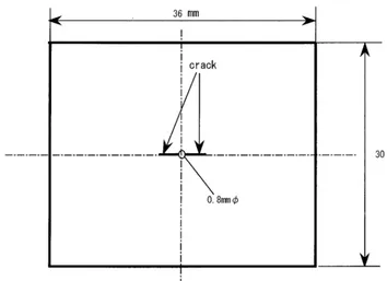
Object of analysis is a center-cracked plate whose dimensions are given in Figure 1. A small circular hole was
allocated at the center of the plate as a crack starter. Along the upper edge of the plate, uniform displacement was given
SMiRT 16, Washington DC, August 2001
Paper # 1693with the average stress cyclically changed between maximum and minimum values as shown in Figure 2. The crack was assumed to initiate at the edge of the hole and grow in the direction perpendicular to the applied load up to 1.85mm in each
side. To simulate crack growth smoothly, 4-noded isotropic elements were used. A large number o f square elements
whose width is 0.05mm were given for the crack plane.
Fourteen cases were analyzed changing maximum and minimum applied stresses. Loading conditions are summarized
in Figure 2. The quantities defined by the following equations using the maximum applied stress, cr ... and the minimum,
o,,,m, were used to characterize the loading condition:
Act = °'max - o'min (1)
2 o 3 ,
O'ma x --I- O"mi n
or,,, = ' (2)
2(0, ... - or,,,,,, )
where cry is the yield stress of the material and Hereafter, they are referred to as normalized stress range and normalized
mean stress, respectively. The temperature was fixed at 550°C, in all cases.
Method of Analysis
Because crack closure behavior is largely affected by plastic deformation, it is necessary to use a constitutive model
which can describe elastic-plastic deformation behavior under cyclic loading with a reasonable accuracy. Classical
constitutive models such as isotropic or linear kinematic hardening model cannot describe the material behavior under cyclic
loading with a sufficient accuracy and their use may bring about predictions which are far from actual behavior. The author
[3] has developed an elastic-plastic constitutive model for austenitic stainless steels aiming at the application to fast breeder
reactor components. The model belongs to a category of two-surface plastic theory and uses a bounding surface outside the
yield surface to represent nonlinear hardening behavior. The model describes the cyclic hardening by expansion of the
bounding surface and temperature-dependent constants were determined for type 304 stainless steel. The model was
incorporated into a finite element program, which was used in the present study.
Crack closure was modeled by using gap elements along crack growth path and extension of crack was simulated by
successively releasing the constraint for dummy nodes. It was done at the minimum stress level to minimize the effect of
local unloading due to change of boundary condition.
Because the current constitutive model can describe cyclic hardening of the material, cycle-by-cycle analysis was
necessary. Calculation using standard material constants was carried out for the first ten loading cycles. Five cycles were
then analyzed by using material constants which accelerate the cyclic hardening to obtain the steady-state cyclic behavior
with less computation time. After the crack extension by nodal release, calculation was carried out for two cycles using
standard material constants before the next crack extension.
Using deformation and stress fields obtained by the finite element analysis, the effective J-integral range, A J e f f , was
numerically evaluated using an equation [3] derived by an analogy to domain integral formulation for the J-integral [4].
Result of Analysis
Examples of stress-strain history obtained by the present analysis are shown in Figure 4. Gradual cyclic hardening as
well as change of stress range accompanying crack extension was simulated realistically.
Variations of crack opening ratio with crack growth are shown in Figure 5 for two typical loading conditions with
different stress ranges. The crack opening ratio is defined as
qo = (°'max - °'open ) / A o"
(3)
(i) Variation of qo with crack growth was relatively small.
(ii) qo increased with the mean stress at constant stress range.
(iii) qo also increased with the stress range at constant stress ratio (normalized mean stress).
D E V E L O P M E N T OF F O R M U L A F O R C R A C K O P E N I N G R A T I O
Range and mean value of remote applied stress have been widely used for expressing the dependency of crack closure
behavior on the loading condition in the past study. However, these parameters lose validity when crack size becomes larger
or applied stress is not simple tension. Here the reference stress defined by the following equation was used for
summarizing the numerical results.
AP (4)
A°"~:t - ( w - 2a)
whereAP is applied load, 14: is plate width and 2a is crack length (including diameter of the circular hole in the present analysis) .
Normalized reference stress obtained by the following equation was used instead of the reference stress itself having
application to other materials in mind.
Acr,.ef
AO're f = ~ (5)
20" 3 ,
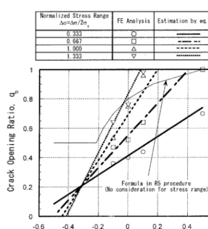
The values of the crack opening ratio at crack growth of 1.65 mm are plotted against the normalized mean stress in
Figure 6 for various normalized stress ranges. It can be seen that the crack opening ratio largely depended on the
normalized stress range as well as the normalized mean stress. At all stress levels, the crack opening ratio increased with
the normalized mean stress almost linearly, and these relations were fitted by the following equations:
qo = 0.27 + 0.37Ao-re f + (0.2 + 1.18Ao're f ) o m (0 < qo < 1) (6)
Predictions given by this equation are in good agreement with independent numerical results as can be seen in Figure 6. A
relation recommended in R5 procedure [5] is also plotted in the figure for comparison. The crack opening ratio given by R5 equation is in relatively good agreement with the results of the present study at higher stress levels but it is considerably larger at low stress level.
E S T I M A T I O N O F E F F E C T I V E J - I N T E G R A L R A N G E
[6].
It is widely known that the J-integral can be predicted by using the reference stress method with a reasonable accuracy According to the method, the total J-integral range is estimated as
EACref
AJtota I = ~ A J e (7)
where Av,.~./ is the strain range corresponding to the reference stress range on a material cyclic stress-strain curve, and E is
the Young's modulus. A J is the elastic J-integral range converted fi'om the elastic stress intensity factor range as.
(AKtotal )2
AJ e = (8)
E
Plastic components of the J-integral range can be separated as
AJp - AJtota ! - AJ e (9)
The effective stress intensity factor range, AKef f can be simply estimated from the total stress intensity factor range,
AKtotal, using the crack opening ratio, q,,.
AKef f = qoAKtotal (1 O)
Then for purely elastic behavior, the following relationship holds:
2 (11)
A Jeff = qo AJtotal
A rigorous relation between the total and the effective J-integral ranges does not exist any more when the plastic zone
size becomes larger and the plastic components of the J-integral range can not be neglected. Budden [7] derived the
following equations which give upper and lower bounds, respectively, for the effective J-integral range:
A Jeff = q 2 A j e + qoAJp (12)
2 qon+l
A Jeff -" qoAJe + AJp
(13)
where n is the exponent which represents dependency of plastic strain range on the stress range.
and 0 _< qo < 1, the following relation always holds"
AJeff (eq. 13 ) <_ AJeff (eq.11) < AJeff (eq. 12 )
Because n>l
Variation of the J-integral with applied stress obtained by the finite element analysis with the domain integration is
shown in Figure 7 for two loading cases. Except the smallest domain that covered only two elements adjacent to the crack
tip, the values were independent of the integration domains. Employing the value at the maximum load at the largest
domain as the effective J-integral range, the numerical results are compared with the estimation by the above equations for five selected crack lengths between 0.25mm and 1.85mm in each loading case.
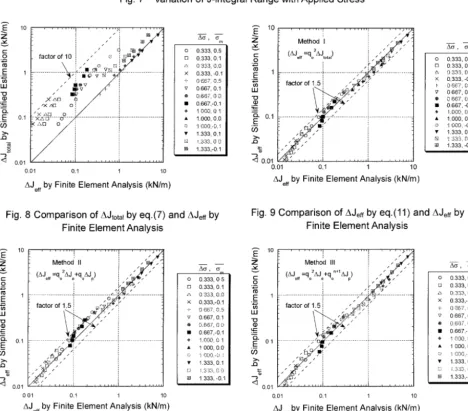
The total J-integral range estimated by eq.(7) is compared with the effective J-integral range evaluated by the domain integration in Figure 8. Values of the total J-integral range estimated by eq.(7) were larger than the numerical results
because of ignorance of crack closure. The amount of overestimation reached about a factor of 10 for the worst case
quite large conservatism in the prediction of crack growth rate.
Then, values of the effective J-integral range estimated by eq,(l 1) through eq,(13) along with the crack opening ratio determined by eq.(6) are compared with the finite element results in Figures 9 to 11. Choice of the equations did not give large difference on the result because of the following reasons:
(i) At lower stress range, crack opening ratio was small but the plastic component of the J-integral range was also small. (ii) At higher stress range, plastic J-integral range was large but the crack opening ratio was also large.
Looking at the results in detail, it can be seen that eq.(11) gave the best agreement with the finite element computations and all points are within a factor of 1.5. This is the simplest equation that holds for the purely elastic condition so that the use of this equation is recommended.
CONCLUSION
Finite element analysis was conducted for a center-cracked plate subjected to cyclic loading to study the fatigue crack
closure under various loading conditions. Based on the results, a simple equation which expresses the dependency of the
crack opening ratio on the range and the mean value of the applied stress was derived. The effective J-integral range
estimated by the simplified method agreed well with the results of finite element analysis. Applicability of the current evaluation method to different loading conditions should be explored in the future.
R E F E R E N C E S
[1] Dowling, N. E. and Begley, J. A., "Fatigue Crack Growth During Gloss Plasticity", ASTM STP 590, 1976, pp. 82-103. [2] Nakayama, Y., Miura, N., Takahashi, Y., Shimakawa, T., Date, S. and Toya Y., "Development of Fatigue and Creep Crack Propagation Law for 316FR Stainless Steel in Consideration of FBR Operating Condition", ASME PVP-Vol.365, 1998, pp. 191-198.
[3] Takahashi, Y., "Development of Inelastic Constitutive Model for Type 304 Stainless Steel and Its Application to Fracture Mechanics Analysis", ASME 1993 Pressure Vessels and Piping Conference, PVP-Vol 262, 1993, pp. 201-208.
[4] Moran, B. and Shih, C. F., "Crack Tip and Associated Domain Integrals from Momentum and Energy Balance", Engineering Fracture Mechanics, Vol. 27, No.6, 1987, pp. 615-642.
[5] Nuclear Electric, "Assessment Procedure for the High Temperature Response of Structures, R5", 1998.
[6] Miller, A. G. and Ainsworth, R. A., "Consistency of Numerical Results for Power-Law Hardening Materials and the Accuracy of the Reference Stress Approximation for J", Engineering Fracture Mechanics, Vol. 32, No.2, 1989, pp. 233-247. [7] Budden, P. J., "Reference Stress Approximations to the AJ Parameter in Cyclic Plasticity", Nuclear Electric Report,
36 mm I
I I i
I i crack
i
|
I O. 8mmq5
i
I
|
I
i
i
|
I
I
i
I i
30 mm
0.6
Fig. 1 Object of Finite Element Analysis
O "node release point
r e m e n t
Fig. 2 Variation of Applied Load
i - - = i - ~ !
~_ 0.4 09
c- 0 . 2
0 c
o
or) t-- - 0 . 2
E
h5
r- - 0 . 4 o Z
- 0 . 6
i i i
r I
- ~ - - - ~ - - m - i - -
I I I
I I I
J ! I ~ I ~ I
I
] ; r
! _ - . . . '
r P i a ~ I '
F
_ ~ - _ _ _
_ _ + _ _ _ _ ~ _ m__~, _~__
!
4 i I , ~ I
I I
]
- - m - . . . i - . . . -ia-~--
i , i i
- - ' - m . . . in . . . Lie
i i
0.5 1 1.5
Nondimensional Stress Range
300 . . . , . . . I . . . A c c e l e r a t i o n of cyclic hardening
200
~
" 100 O 4z o
b -100
-200 -i ...
-300 I , , , , , , , -0.005
300
200
100
z o
b~ -100
. . . 200
-300
0 0.005 0.01 -0.005 0 0.005 0.01 0.015 0.02 0 . 0 2 5
(mm/mm) ~ (mm/mm)
YY yy
(a) Integration point nearest to hole edge (x=O. 41 mm, y=O. 01 mm)
(b) Integration point far from the hole (x=1.41 mm,y=O. 01 mm)
Fig. 4 Example of Stress-Strain History (for the case of Act = 1, o% = 0)
1.2
1
d • - 4 - 1 0 . 8 t Y
b . O E 0 . 6 E Q o 0 . 4
° 0.2
i i i | , , i i i ! | | i | ! |
Aa=O. 663
. . . 0 - - - - 0 4 - - - 0 . 0 0 - - - _ _ . . .
_ __._----q3 - _ _ _ _ _ _ _ _ . ~ _ - - - ~
. . . ~ ' ~ . . . ,/~ - A ~ "
, ~
, ~
,
... ! ... % ... i ... ! ... - - o - - 0.5 I i i - - - ~ - - O. l l i i
... ~ 0 . 0 1 ...
- ~ v - ~ -0. I I
I I I I I I I I I I I I I I I I I
0 . 5 1.5
Crack Growth (mm)
Normalized Stress Range
Aa=Aa/2a FE Analysis Estimation by eq. (8) y
0.333 O
0.667 [] 1. 000 /k
1. 333 ~ ...
1
D ° 0.8 d
r~, 0.6
c~ 0.4
O o 0.2
0 -0.6
I : ] • ,
: : i," , ' i
! ! :/ • • :
D
i i o
i" • ! !
~ # ' j : : : . . . i . . . ""~-~ "#- ' ~ " - . . . " . . . J . . .
'
~ ,
,,Formula in R5 procedure (No consideration for stress range)--
I I
-0.4 -0.2 0 0.2 0.4
N o r m a l i z e d Mean S t r e s s , ~ m = ~ m / A ~ 0.6
Fig. 5 Example of Variation of Crack Opening Ratio with Crack Growth
0 . 0 0 2 . . . . ~ . . . . I . . . . ! . . . . I . . . .
Case C (Ao-=0.333, ~m=0.0)
..-, Crack growth: 0.45mm
E 0.0015 IArea Integration Region I , . . . i
i ---I~-- 2 , . . . " . . . ~ 3 ' i
x 4
&
0.001 n~
0.0005
0
- 1 0 0 10 20 30 4 0
Applied Stress (MPa)
( a ) A o - = 0 . 3 3 3 , o-,,, = 0 . 0 ,
crack growth'O.45mm
u . ] o . . . . t . . . . I . . . . I . . .
Case
J ( A ~ = I . 0 0 0 , ~ = 0 . 0 )m
.... Crack growth 1.25mm
"~ i x 4 i
o~ 0.05 . . .
!.--
0 i i , i i i i i i i i
- 1 0 0 - 5 0 0 5 0 1 0 0 1 5 0
Applied Stress (MPa)
(b)
A o - = 1 . 0 0 , G,,, = 0 . 0 ,crack growth'l.25mm
Fig. 7 Variation of J-integral Range with Applied Stress
..EE lO
z
(-- O
E 1
. _ UJ "O (l) . _ EL E 0.1 . _
09
> , _O
<1 OOl
,. ; [] i
/ / (i
f a c t o r of 10 ,-" ,:.~; i ~ [ ] ~ ' ... - ~ i ~ - ~ i ...
: b
-×A~ o J
::
- ~ ... - o - - - 7 ~ ...
I I I I I I I I I i I I I I I I I I I I I I I I I
0.01 0.1 1 10
A Jeff by Finite Element Analysis (kN/m)
m o 0.333, 0.5 [] 0.333, 0.1
z.',. 0 333, 0.0
x 0.333, -0.1 -~- 0 667, 0.5 ~/ 0.667, 0.1
0.667", 0 0
• 0.667,-0.1 ~, 1 000, 0 1
A 1.000, 0.0
,~, I 000,.0. ! • 1.333, 0.1 ~:-J ~,.333, 0 0 [] 1.333,-0.1
~" 10
z
v ( - O
E 1
(/) LU "O
~
- 0.1 09_(3
<3 0.01 0.01
... ... ,
Method '1 ;; , ~ . , - !
( A Jeff =qo2AJtotal) ~ / ,-
... factor ofl.5 i ...
I I S -~~'-
-"-~,-':- . . . ...-
::" , . . . :: . . .
1
1
0.1 1 10
AJef f by Finite Element Analysis (kN/m)
AO" 7 (3'
m o 0.333, 0.5 13 0.333, 0 1 #. 0 333, 0.0 x 0.333, -0.1 0 667, 0 5 ~7 0 667, 0.1 0 667, 0 0 • 0.667, -0.1 1.000, C. 1 A 1.000, 0.0 ~:~. I 0 0 0 , - 0 1 • 1.333, 0.1
1 3 3 3 . 0 . 0 [] 1.333, -0.1
Fig. 8 Comparison of AJtota I by eq.(7) and AJef f by Finite Element Analysis
Fig. 9 Comparison of A Jeff by eq.(11) and A Jeff by Finite Element Analysis
,~- lO . . . ! . . . , , ,
M e t h o d ' II ', , , ~
ii
1 ... ! ... ~':.-.--
~j factor of 1.51 ~ ' : . v ~ " 1
EL 0.1
o5
d
0.01
0 0 1 0.1 1 10
AJef f by Finite Element Analysis (kN/m)
Ao- , (3"
o 0.333, 0 5 [] 0.333, 0.1 z.~ 0 333,010 x 0.333,-0.1 { 0 667, 0.5 v 0.667, 0.1 0.66?', 0 0 • 0.667,-0.1 1.000, 0 1 A 1 000, 0.0 "i 000,- {;. • 1.333, 0.1
! 3 3 3 . 0 0 [] 1 333,-0.1
~
" 10 Z v E OE 1
(/) LU "O (l) . _ I
~ - 0 1
O9 J3 <3 0.01 0.01 , , . . . ! . . . ! ' , , ) , , ,
M e t h o c l III , ,- . ~ , ,
(AJef f = q o 2 A J e + q o n+IAJP) , . ~ ,, /
',
,!" ;tl ...
... factor of 1.5!i ... i : ~ ~ [ . >-",.~ ~ ...
: : v " , - :: /,~ / /
0.1 1 10
AJef f by Finite Element Analysis (kN/m)
/ ~ , G"
m o 0.333, 0.5 [] 0.333, 0 1 ,':: 0.333, 0 0 x 0.333,-0.1 + ,'3 ..!"67.0.5 v 0 667, 0.1 • 0.66.;', 0 0 I 0.667,-0 1 I 000, 0 1 A, 1 000, 0.0 ',:: i 000,-0 ! • 1.333, 0.1 .,'-; ~.333, C.' 0 [] 1.333,-0 1
Fig. 10 Comparison of A Jeff by eq.(12) and A Jeff by Finite Element Analysis