NN-Harmonic Mean Aggregation Operators Based MCGDM Strategy in Neutrosophic Number Environment

(1)

Article

1

NN-Harmonic Mean Aggregation Operators Based

2

MCGDM Strategy in Neutrosophic Number

3

Environment

4

Kalyan Mondal 1_{, Surapati Pramanik}2,_{*, Bibhas C. Giri}3_{and Florentin Smarandache}4

5

1 _{Department of Mathematics, Jadavpur University, West Bengal, India.}

6

Email: [email protected]

7

² Department of Mathematics, Nandalal Ghosh B.T. College, Panpur, PO-Narayanpur, and District: North 24

8

Parganas, Pin Code: 743126, West Bengal, India. Email: [email protected]

9

3 _{Department of Mathematics, Jadavpur University, West Bengal, India.}

10

11

4 _{University of New Mexico, Mathematics & Science Department, 705 Gurley Ave., Gallup, NM 87301, USA.}

12

13

* Correspondence: [email protected]; Tel.: +919477035544; Phone no: +91-33-25601826;

14

Fax no: +91-33-25601826

15

Abstract: The concept of neutrosophic number is a significant mathematical tool to deal with real

16

scientific problems because it can tackle indeterminate and incomplete information which exists

17

generally in real problems. In this article, we use neutrosophic numbers (a + bI), where a and bI

18

denote determinate component and indeterminate component respectively. We explore the

19

situations in which the input information is needed to express in terms of neutrosophic numbers.

20

We define score functions and accuracy functions for ranking neutrosophic numbers. We then

21

define a cosine function to determine unknown criteria weights. We define neutrosophic number

22

harmonic mean operators and proved their basic properties. Then, we develop two novel MCGDM

23

strategies using the proposed aggregation operators. We solve a numerical example to demonstrate

24

the feasibility and effectiveness of the proposed two strategies. Sensitivity analysis with variation

25

of “I” on neutrosophic numbers is performed to demonstrate how the preference ranking order of

26

alternatives is sensitive to the change of “I”. The efficiency of the developed strategies is

27

ascertained by comparing the obtained results from the proposed strategies with the existing

28

strategies in the literature.

29

Keywords: neutrosophic number; neutrosophic number harmonic mean operator (NNHMO);

30

neutrosophic number weighted harmonic mean operator (NNWHMO); cosine function, score

31

function; multi criteria group decision making

32

33

1. Introduction

34

Multi-criteria group decision making (MCGDM) is a significant branch of decision theory

35

which has been commonly applied in many scientific fields such as medical diagnosis [1, 2], decision

36

making [3, 4], supplier selection [5], etc. Because of the indeterminate information and the

37

complexity of decision problems, it is difficult to express criteria in terms of crisp numbers. To tackle

38

the difficulty, neutrosophic number (NN) [6, 7] is proposed in the literature. The NN consists of

39

determinate component and an indeterminate component. So the NNs are more practical to deal

40

with indeterminate and incomplete information in real world problems. The NN is expressed as the

41

(2)

function N = p + qI in which p is the determinate component and qI is the indeterminate component. If

42

N = qI i.e. the indeterminate part reaches the maximum label, the worst situation occurs. If N = p i.e.

43

the indeterminate part does not appear, the best situation occurs. Thus, application of NNs is more

44

appropriate to deal with the indeterminate and incomplete information in practical decision making

45

situations.

46

Information aggregation is an essential practice of accumulating relevant information from

47

various sources. Harmonic mean is the reciprocal property of arithmetic mean. It is used to present

48

for aggregation between the min and max operators. Harmonic mean is usually used as a

49

mathematical tool to accumulate central tendency of information.

50

The harmonic mean (HM) is widely used in statistics to calculate central tendency of a set of data.

51

Park et al. [8] proposed multi-attribute group decision making (MAGDM) strategy based on HM

52

operators under uncertain linguistic environment. Wei [9] proposed MAGDM strategy based on

53

fuzzy induced ordered weighted HM. In fuzzy environment, Xu [10] studied fuzzy weighted HM

54

operator, fuzzy ordered weighted HM operator, and fuzzy hybrid HM operator and employed them

55

for MADM problems. Ye [11] proposed multi-attribute decision making (MADM) strategy based on

56

harmonic averaging projection for simplified neutrosophic sets (SNS) environment.

57

In NN environment, Liu and Liu [12] proposed NN generalized weighted power averaging operator

58

for MAGDM. Zheng et al. [13] proposed MAGDM strategy based on NN generalized hybrid

59

weighted averaging operator. Pramanik et al. [14] studied teacher selection strategy based on

60

projection and bidirectional projection measures in NN environment.

61

Literature review reflects that MCGDM strategy using NNs has made little progress in real

62

scientific and engineering fields. Therefore, it is necessary to explore new strategies to handle

63

MCGDM problems in NN environment.

64

In this paper, we develop two MCGDM strategies based on neutrosophic number harmonic

65

mean operator (NNHMO) and neutrosophic number weighted harmonic mean operator

66

(NNWHMO) to solve MCGDM problems. The proposed strategies can handle the indeterminacy of

67

information.

68

The paper is sequenced as follows. Section 2 presents some preliminaries of NNs and score

69

and accuracy functions of NNs. Section 3 devotes NN harmonic mean operator (NNHMO) and NN

70

weighted harmonic mean operator (NNWHMO). Section 4 defines cosine function to determine

71

unknown criteria weights. Section 5 presents two novel decision making strategies based on

72

NNHMO and NNWHMO. In section 6, a numerical example is presented to illustrate the proposed

73

MCGDM strategies and the results show the feasibility of the proposed MCGDM strategies. Section

74

7 compares the obtained results derived from the proposed strategies and the existing strategies in

75

NN environment. Finally, Section 8 concludes the paper with some remarks and future scope of

76

research.

77

2. Preliminaries

78

In this section, the concepts of NNs, operations on NNs, score and accuracy functions of NNs

79

are outlined.

80

2.1. NNs [5, 6]

81

NN consists of a determinate component x and an indeterminate component yI, and

82

mathematically is expressed as z = x + yI for x, y∈R, where I is indeterminacy interval and R is the set

(3)

of real numbers. A NN z can be specified as a possible interval number, denoted by z = [x + yIL_,_{x +}

84

yIU_{] for}_z∈_Z₍_Z_{is set of all NNs) and}_I∈_[_IL_{, I}U_{]. The interval}_I∈_[_IL_{, I}U_{] is considered as an}

85

indeterminate interval.

86

• If yI = 0, then z is degenerated to the determinate component z = x

87

• If x = 0, then z is degenerated to the indeterminate component z = yI

88

• If IL₌_IU_{, then}_z_{is degenerated to a real number.}

89

Let two NNs be z1 = x1+ y1I and z2 = x2 + y2I for z1, z2∈Z, and I∈[IL, IU]. Some basic operational

90

rules for z1 and z2 are presented as follows:

91

(1) I2₌_I

92

(2) I.0 = 0

93

(3) I/I = Undefined

94

(4) z1 + z2 = x1 + x2 + (y1 + y2)I = [x1 + x2 + (y1 + y2)IL, x1 + x2 + (y1 + y2)IU]

95

(5) z1 −z2 = x1−x2 + (y1 −y2)I = [x1 −x2 + (y1 −y2)IL, x1−x2 + (y1 −y2)IU]

96

(6) z1×z2 = x1x2 + (x1y2 + x2y1)I + y1y2I2 = x1x2 + (x1y2 + x2y1 + y1y2)I

97

(7) =

z z

2

1 ₌

I y + x

2 2

1 1

2 2 y x x I y x x

y x y x x x

− ≠ ≠ +

−

+ ; 0,

)

( ₂ ₂ 2

2

2 1 1 2 2 1

98

(8) =

z1

1

= I y + x

I. +

1 1

0 1

1 1 1 1 1 1

1

, 0 ; ) (

1 _I _x _x _y

y x x

y

x ₊ ≠ ≠−

− +

99

(9) z12=x12+(2x1y1+y12)I

100

(10) λz1=λx1+λy1I

101

102

Definition 1. For any NN z = x + yI = [x + yIL_,_{x + yI}U_{], (}_x_and_y_{not both zeroes), its score and accuracy}

103

functions are defined, respectively, as follows:

104

y x

I I y x z

S U L

2 2

2

) ( )

(

+ − +

= (1)

105

) (

exp 1 )

(z x y IU IL

A = − − + − (2)

106

Theorem 1. Both score function S(z) and accuracy function A(z) are bounded.

107

Proof.

108

x, y∈R and I∈[0, 1], 0 1

2

2₊ ≤

≤ y x

x

,0 ( ) 1

2

2₊ ≤

− ≤

y x

I I

y U L

109

 0 ( ) 2

2

2₊ ≤

− + ≤

y x

I I y

x U L

 1

2

) ( 0

2

2₊ ≤

− + ≤

y x

I I y

x U L

 0≤S(z)≤1.

110

Since0 ≤S(z)≤ 1, score function is bounded.

111

Again,

112

1 ) ( exp

0≤ − _x+_y _IU −_IL ≤ _₋₁_≤ ₋_exp ₋_x₊_y₍_IU ₋_IL₎ _≤₀ _₀_≤₁₋_exp ₋ _x₊_y₍_IU ₋_IL₎ _≤₁

113

Since−1≤A(z)≤ 1, accuracy function is bounded.

(4)

Definition 2. Let two NNs be z1 = x1+y1I = [x1+y1IL, x1+y1IU], and z2 = x2+y2I = [x2+y2IL, x2+y2IU], then the

115

following comparative relations hold:

116

• If S(z1) > S(z2), then z1 > z2

117

• If S(z1) = S(z2) and A(z1) < A(z2), then z1 < z2

118

• If S(z1) = S(z2) and A(z1) = A(z2), then z1 = z2.

119

Example 1. Let three NNs be z1 = 10 + 2I, z2 = 12 and z3 = 12 + 5I and I∈[0, 0.2]. Then,

120

S(z1) = 0.5099, S(z2) = 0.5, S(z3) = 0.5577, A(z1) = 0.999969, A(z2) = 0.999994, A(z3) = 0.999997.

121

We see that,S(z₁)S(z₂)=S(z₃), andA(z₃)S(z₂).

122

Using definition 2, we conclude that,z1 z3z2.

123

3. NN- harmonic mean operator (NNHMO)

124

Definition 3. Let zi = xi + yiI (i = 1, 2, …, n) be a collection of NNs. Then the NNHMO is defined as

125

follows:

126

) , , ,

NNHMO(z₁ z₂ z_n =

( )

1 1 1 . − = − _     

_

n

i i

z

n (3)

127

Theorem 2. Let zi = xi + yiI (i = 1, 2, …, n) be a collection of NNs. The aggregated value of the

128

) , , ,

NNHMO(z1 z2 zn operator is also a NN.

129

Proof. NNHMO(z1,z2,,zn) =

( )

1 1 1 . − = − _     

_

n

i i

z n

130

= i i i

n

i i i i

i i y x x I y x x y x

n _ ≠ ≠−

     + − + − =



; 0,

) ( 1 . 1 1

131

= i i i

n

i n

i _i _i _i i i y x x I y x x y x

n _ ≠ ≠−

     + − + − = =



; 0,

) ( 1 . 1 1 1

132

= i i i

n

i n

i _i _i _i i i y x x I y x x y x

n _ ≠ ≠−

     + − + − = =



; 0,

) ( 1 . 1 1 1

133

=



= = = = = = = = + − − ≠ ≠       + − +       + − − + n

i _i _i _i i n i _i n i _i n

i _i _i _i i n i _i y x x y x x I y x x y x x y x x y n x n 1 1 1 1 1 1 1 1 ) ( 1 , 0 1 ; ) ( 1 1 ) ( . 1

134

It shows that NNHMO is also a NN.

135

Definition 4. Let zi = xi + yiI (i = 1, 2, …, n) be a collection of NNs. Then the NN- weighted harmonic

136

mean (NNWHMO) is defined as follows:

137

) , , ,

NNWHMO(z1 z2 zn =

( )

1 1 1 . − = −      

_

n

i i i

z

w

(4)

138

Theorem 3. Let zi = xi + yiI (i = 1, 2, …, n) be a collection of NNs. The aggregated value of the

139

) , , ,

NNWHMO(z1 z2 zn operator is also a NN.

(5)

Proof. NNWHMO(z1,z2,,zn)=

( )

1 1 1 . − = −      

_

n

i i i

z

w

142

= i i i

n

i _i _i _i

i

i _x _x _y I x x y

y x

w

_ ≠ ≠−

            + − + − =



; 0,

) (

1 1

1

143

= i i i

n

i

n

i _i _i _i i i

i

i _x _x _y I x x y

y

x

w

_ ≠ ≠−

     + − + − = =



; 0,

) ( . 1 . 1 1 1

144

= ; 1

) ( . 1 . , 0 1 . ; ) ( . 1 . 1 . ) ( . 1 . 1 1 1 1 1 1 1 1 1 1 = + − − ≠ ≠       + − +       + − − +



= = = = = = = = = n i i n

i _i _i _i i i n i _i i n i _i i n

i _i _i _i i i n i i i

w

x x y

y x x I y x x y x x y x x y x .

145

It shows that NNWHMO is also a NN.

146

Example 2. Let two NNs be z1 = 3 + 2I and z2 = 2+ I and I∈[0, 0.2]. Then,

147

) , NNHMO(z1 z2 =

1 2 1 1 1 2 −         + z z = 1 2 1 2 3 1 2 −       + +

+ I I = 2.4 + 0.635I.

148

Example 3. Let two NNs be z1 = 3 + 2I and z2 = 2 + I, I∈[0, 0.2] and w1 = 0.4, w2 = 0.6, then,

149

) , NNWHMO(z1 z2 =

1 2 2 1 1 1 1 −         + z w z w = 1 2 1 6 . 0 2 3 1 4 . 0 −       + +

+ I I =2.308 + 1.370I.

150

The NNHMO operator and the NNWHMO operator satisfy the following properties.

151

P1. Idempotent law: If zi = z for i = 1, 2, …, n then, NNHMO(z₁,z₂,,z_n)=z and

152

z z z

z, , , n)=

NNWHMO( 1 2

153

Proof. For, zi = z,

154

) , , ,

NNHMO(z1 z2 zn =

( )

1 1 1 . − = − _     

_

n

i i

z

n =

( )

1 1 1 . − = − _     

_

n

i

z

n = ₁

._z− n

n

= z.

155

) , , ,

NNWHMO(z1 z2 zn =

( )

1 1 1 . − = −      

_

n

i i i

z

w

=

( )

1 1 1 . − = −      

_

n

i i

z

w

=

( )

1 1 1 1 . . − − − =    



_

n _z

i

w

i = z.

156

P2. Boundedness: Both the operators are bounded.

157

Proof. Ifz_min=min(z₁,z₂,,z_n), z_max=max(z₁,z₂,,z_n)for i = 1, 2, …, n then,

158

max 2

1

min NNHMO(z,z , ,z ) z

z ≤  n ≤ andzmin≤ NNWHMO(z1,z2,,zn)≤zmax.

159

P3. Monotonicity: Ifzi≤zi*for i = 1, 2, …, n then, NNHMO( , , , ) NNHMO( , *2, , *)

* 1 2

1 z zn

z

n

z  ≤  and

160

) , , , NNWHMO( ) , , ,

NNWHMO( * *

2 * 1 2

1 z zn

z

n

z  ≤  .

161

(6)

Proof_. NNHMO( , , , ) NNHMO( , *2, , *) *

1 2

1 z zn

z

n

z  − 

163

=

( )

1 1 1 * 1 1 1 _. . − = − − = − _      −     



_

n i i n i i z n z

n ≤0, forzi≤zi*, for i = 1, 2, …, n.

164

Again,

165

) , , , NNWHMO( ) , , ,

NNWHMO( * *

2 * 1 2

1 z zn

z

n

z  − 

166

=

( )

1 1 1 * 1 1 1 . . − = − − = −       −     



_

n i i i n

i i i

z

_w

w

≤0, forzi≤zi*( i = 1, 2, …, n).

167

This proves the monotonicity of the functionsNNHMO(z1,z2,,zn)andNNWHMO(z1,z2,,zn).

168

P4. Commutativity: If(z1,z2,,zn)be any permutation of (z1,z2,,zn)then,

169

) , , , NNHMO( ) , , ,

NNHMO(z₁ z₂_ z_n ₌

_z

₁

_z

₂_

_z

_n

andNNWHMO(z1,z2, ,zn) NNWHMO(

z

1,

z

2, ,

z

n)

 

 _

 =

170

Proof. NNHMO(z1,z2,,zn) − NNHMO(

z

1,

z

2,,

z

n)

171

=

( )

1 1 1 * 1 1 1 _. . − = − − = − _      −     



_

n i i n i i z n z

n = 0, because, (z1,z2,,zn)is any permutation of(z1,z2,,zn).

172

Hence, we haveNNHMO(z1,z2, ,zn) NNHMO(

z

1,

z

2, ,

z

n)

   _  = .

173

Again,

174

) , , , NNWHMO( ) , , ,

NNWHMO(z₁z₂_ z_n ₋

_z

₁

_z

₂_

_z

_n

175

=

( )

1 1 1 * 1 1 1 . . − = − − = −       −     



_

n i i i n

i i i

z

_w

w

= 0, because, (z1,z2,,zn)is any permutation of(z1,z2,,zn).

176

Hence, we haveNNWHMO(z1,z2, ,zn) NNWHMO(

z

1,

z

2, ,

z

n)

 

 _

 ₌ .

177

4. Cosine function for determining unknown criteria weights

178

When criteria weights are completely unknown to decision makers, the entropy measure [15] can be

179

used to calculate criteria weights. Biswas et al. [16] employed entropy measure for MADM problems

180

to determine completely unknown attribute weights of single valued neutrosophic sets (SVNSs).

181

Literature review reflects that, strategy to determine unknown weights in NN environment is yet to

182

appear. In this paper, we propose a cosine functionto determine unknown criteria weights.

183

Definition 5. The cosine functionof a NN P= xij + yijI = [xij + yijIL, xij + yijIU], (i = 1, 2, ..., m; j = 1, 2, ..., n) is

184

defined as follows:

185

          +  π =

= _x _y

y n P COS ij ij ij n i j 2 2 1cos2 1

)

( , (xij and yij are not both zeroes) (5)

186

The weight structure is defined as follows.

(7)

 =

= n

j j

P COS

P COS w

1 ( )

) (

; j = 1, 2, ..., n & 1

1 =

 =

n

j wj (6)

188

The cosine function COSj(P)satisfies the following properties:

189

P1. COSj(P)=1, if yij=0.

190

P2. COSj(P)=0, if xij=0

191

P3. COSj(P)≥COSj(Q), if xij of P > xij of Q or yij of P < yij of Q or both.

192

Proof.

193

P1. y_ij=0 ( ) 1

[

cos0

]

1

1 =

 =

= n

i j

n P COS

194

P2. xij=0  cos₂ 0

1 ) (

1 =

_ π_

=

= n

i j

n P COS

195

P3. For, xij of P > xij of Q

196

Determinate part of P > Determinate part of Q

197

 COSj(Q)<COSj(P).

198

For, yij of P < yij of Q

199

Indeterminacy part of P < Indeterminacy part of Q

200

 COSj(Q)>COSj(P).

201

For, xij of P > xij of Q and yij of P < yij of Q

202

 (Real part of P > Real part of Q) & (Indeterminacy part of P < Indeterminacy part of Q)

203

 COSj(Q)>COSj(P).

204

Example 4. Let twoNNs be z1 = 3 + 2I, and z2 = 3 + 5I, then,COS(z₁)=0.9066,COS(z₂)=0.7817.

205

Example 5. Let twoNNs be z1 = 3 + I, and z2 = 7 + I, then,COS(z₁)=0.9693,COS(z₂)=0.9938.

206

Example 6. Let twoNNs be z1 = 10 + 2I, and z2 = 2 + 10I, then, COS(z₁)=0.9882,COS(z₂)=0.7178.

207

5. Multi-criteria group decision making strategies based on NNHMO and NNWHMO

208

Two MCGDM strategies using the NNHMO and NNWHMO respectively are developed in this

209

section. Suppose that L = {L1, L2, . . . , Lm} is a set of alternatives, C = {C1, C2, . . . , Cn} is a set of criteria

210

and DM = {DM1, DM2, . . . , DMk} is a set of decision makers. Decision makers’ assessment for each

211

alternative Li will be based on each criterion Cj. All the assessment values are expressed by NNs.

212

Steps of decision making strategies based on proposed NNHMO and NNWHMO to solve MCGDM

213

problems are presented as follows.

214

5.1. MCGDM Strategy 1 (based on NNHMO)

215

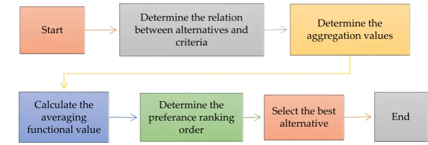
The strategy 1 is presented (see Figure 1) using the following six steps.

216

(8)

Step 1.Determine the relation between alternatives and criteria

218

Each decision maker forms a NN decision matrix. The relation between the alternative Li (i = 1, 2, ...,

219

m)and the criterion Cj (j = 1, 2, ..., n) is presented in Table 1.

220

221

Table 1. The relation between alternatives and criteria in terms of NNs

222

     

 

     

 

+ +

+

+ +

+

+ +

+ =

k mn mn k

m m k m m

k n n k

k

k n n k

k

n

m k

I y x I

y x I y x

I y x I

y x I y x

I y x I

y x I y x

C C

C

L L L C L

DM

2 2 1

1

2 2 22

22 21

21

1 1 12

12 11

11

2 1

2 1 ] | [

  



  



223

Here, xij+yijI krepresents the NN rating value of the alternative Li with respect to the criterion Cj

224

for the decision maker DMk.

225

Step 2.Using Eq. (3), determine the aggregation values (DMaggrk(Li)), (i = 1, 2, …, n) for all decision

226

matrices.

227

Step 3.To fuseall the aggregation values (DMaggr_k(L_i)), corresponding to alternatives Li, we define

228

the averaging function as follows.

229

k L DM L

DM

k

t i

aggr k i

aggr₍ ₎ ₌ =1 ( )

(i = 1, 2, …, n) (7)

230

Step 4.Determine the preference ranking order

231

Using Eq. (1), determine the score values S(zi) (accuracy degrees A(zi), if necessary) (i = 1, 2, . . . ,

232

m) of all alternatives Li. All the score values are arranged in descending order. The alternative

233

corresponding to the highest score value (accuracy values) reflects the best choice.

234

Step 5.Select the best alternative from the preference ranking order.

235

Step 6. End.

236

237

Figure 1. Steps of MCGDM strategy 1 based on NNHMO.

238

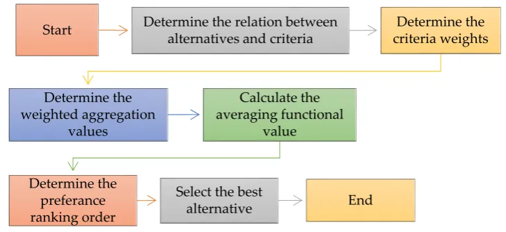
5.2. MCGDM Strategy 2 (based on NNWHMO)

239

The strategy 2 is presented (see Figure 2) using the following seven steps.

240

Step 1.This step is similar to the first step of strategy 1.

241

Step 2.Determine the criteria weights

242

Start

Determine the relation between alternatives and

criteria

Determine the aggregation values

Calculate the averaging functional value

Determine the preferance ranking

order

Select the best

(9)

Using Eq. (6), determine the criteria weights from decision matrices (DMt[L|C]), (t = 1, 2, ..., k).

243

Step 3.Determine the weighted aggregation values (DMwaggrk(Li))

244

Using Eq. (4), determine the weighted aggregation values (DMwaggrk(Li)), (i = 1, 2, …, n) for all

245

decision matrices.

246

Step 4.Determine the averaging values

247

To fuse all the weighted aggregation values (DMwaggrk(Li)), corresponding to alternatives Li, we

248

define the averaging function as follows.

249

k L DM L

DM

k

t i

waggr k i

aggr₍ ₎ ₌ =1 ( )

(i = 1, 2, …, n) (8)

250

Step 5.Determine the ranking order

251

Using Eq. (1), determine the score values S(zi) (accuracy degrees A(zi), if necessary) (i = 1, 2, . . . ,

252

m) of all alternatives Li. All the score values are arranged in descending order. The alternative

253

corresponding to the highest score value (accuracy values) reflects the best choice.

254

Step 6Select the best alternative from the preference ranking order.

255

Step 7 End.

256

257

258

259

Figure 2. Steps ofMCGDM strategy based on NNWHMO.

260

6. Simulation results

261

We solve a numerical example studied by Zheng et al. [13]. An investment company desires to

262

invest a sum of money in the best investment fund. There are four possible selection options to

263

invest the money. Feasible selection options are namely, L1: Car company (CARC), L2: Food company

264

(FOODC), L2: Computer company (COMC), L4: Arms company (ARMC). Decision making must be

265

based on the three criteria namely, Risk analysis (C1), Growth analysis (C2), Environmental impact

266

analysis (C3). The four possible selection options/alternatives are to be selected under the criteria by

267

the NN assessments provided by the three decision makers DM1, DM2, DM3.

268

Start Determine the relation between

alternatives and criteria

Determine the criteria weights

Determine the weighted aggregation

values

Calculate the averaging functional

value

Determine the preferance ranking order

Select the best

(10)

6.1. Solution using MCGDM Strategy 1

269

Step 1.Determine the relation between alternatives and criteria.

270

All assessment values are provided by the following three NN based decision matrices (shown in

271

Tables 2, Table 3, and Table 4).

272

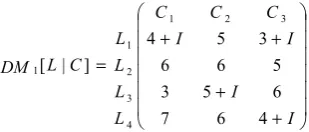
Table 2. NN based decision matrix for DM1

273

                + + + + = I I I I C C C L L L L C L DM 4 6 7 6 5 3 5 6 6 3 5 4 ] | [ 3 2 1 4 3 2 1 1

274

275

                + + + = 5 6 6 5 5 4 6 6 5 4 4 5 ] | [ 3 2 1 4 3 2 1 2 I I I C C C L L L L C L DM

276

277

                + + + + = I I I I C C C L L L L C L DM 4 6 8 6 5 4 5 7 6 4 5 4 ] | [ 3 2 1 4 3 2 1 3

278

Step 2.Determine the weighted aggregation values ( aggr( _i)

k L

DM )

279

Using Eq. (3), we calculate the aggregation values ( aggr( _i)

kL

DM ) as follows:

280

I L

DMaggr₍ ₎ ₃_.₈₂₉ ₀_.₇₈₅ 1

1 = + ;DMaggr1(L2)=5.625;DMaggr1(L3)=4.285+0.214I;DMaggr1(L4)=5.362+0.514I;

281

285 . 4 ) ( ₁

2L =

DMaggr

;DMaggr₍L ₎ ₅_.₂₀₆ ₀_.₄₁₅I

2

2 = + ;DMaggr2(L3)=4.196+0.532I;DMaggr2(L4)=5.234+0.618I;

282

I L

DMaggr₍ ₎ ₄_.₀₁₉ ₀_.₆₀₅ 1

3 = + ;DMaggr3(L2)=5.817+0.433I;DMaggr3(L3)=4.876+0.387I

283

I L

DMaggr₍ ₎ ₆_.₀₂₃ ₀_.₂₅₇ 4

3 = + .

284

285

Using Eq. (7), we calculate the averaging values to fuseall the aggregation values corresponding to

286

the alternative Li.

287

I L

DMaggr₍ ₎ ₄_.₀₄₄ ₀_.₄₆₃

1 = + ;DMaggr(L2)=5.549+0.282I;DMaggr(L3)=4.452+0.378I;

288

I L

DMaggr₍ ₎ ₅_.₅₃₉ ₀_.₄₆₃

4 = + .

289

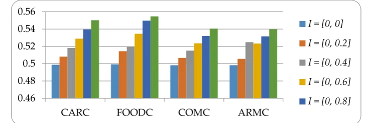
Step 4.Using Eq. (1), we calculate the score values S(Li) (i = 1, 2, 3, 4). Score values and ranking of

290

alternatives for different values of “I” are shown in Table 5.

291

(11)

Table 5. Ranking order with variation of “I” on NNsfor strategy 1

293

294

I S(Li) Ranking order

I =[0, 0] S(L1) = 0.4988, S(L2) = 0.4993, S(L3) = 0.4982, S(L4) = 0.4983 L2L1L4L3 I∈[0, 0.2] S(L1) = 0.5081, S(L2) = 0.5144, S(L3) = 0.5067, S(L4) = 0.5056 L2L1L3L4 I∈[0, 0.4] S(L1) = 0.5182, S(L2) = 0.5195, S(L3) = 0.5151, S(L4) = 0.5249 L2L1L4L3 I∈[0, 0.6] S(L1) = 0.5289, S(L2) = 0.5346, S(L3) = 0.5236, S(L4) = 0.5233 L2L1L3L4 I∈[0, 0.8] S(L1) = 0.5396, S(L2) = 0.5497, S(L3) = 0.5320, S(L4) = 0.5316 L2L1L3L4 I∈[0, 1] S(L1) = 0.5503, S(L2) = 0.5547, S(L3) = 0.5405, S(L4) = 0.5399 L2L1L3L4

295

Step 5.Food company (FOODC)is the best alternative for investment.

296

Step 6.End

297

298

299

300

301

302

303

304

305

6.2. Solution using MCGDM Strategy 2

306

Step 1.Determine the relation between alternatives and criteria

307

This step is similar to the first step of strategy 1.

308

Step 2.Determine the criteria weights

309

Using Eqs. (5) and (6), criteria weights are calculated as follows:

310

[w1 = 0.3265, w2 = 0.3430, w3 = 0.3305] for DM1,

311

[w1 = 0.3332, w2 = 0.3334, w3 = 0.3334] for DM2,

312

[w1 = 0.3333, w2 = 0.3335, w3 = 0.3332] for DM3.

313

Step 3.Determine the weighted aggregation values (DMwaggrk(Li))

314

Using Eq. (4), we calculate the aggregation values ( aggr( _i)

kL

DM ) as follows:

315

I L

DMaggr₍ ₎ ₃_.₈₆₁ ₀_.₇₇₄ 1

1 = + ;DMaggr1(L2)=6.006;DMaggr1(L3)=4.307+0.234I;DMaggr1(L4)=5.399+0.541I;

316

288 . 4 ) ( ₁

2L =

DMaggr

;DMaggr₍L ₎ ₅_.₂₁₉ ₀_.₄₂₉I

2

2 = + ;DMaggr2(L3)=4.206+0.541I;DMaggr2(L4)=5.251+0.629I;

317

I L

DMaggr₍ ₎ ₄_.₀₂₄ ₀_.₆₁₆ 1

3 = + ;DMaggr3(L2)=5.824+0.445I;DMaggr3(L3)=4.889+0.393I; DMaggr3(L4)=6.029+0.265I.

318

319

320

0.46 0.48 0.5 0.52 0.54 0.56

CARC FOODC COMC ARMC

I = [0, 0]

I = [0, 0.2]

I = [0, 0.4]

I = [0, 0.6]

I = [0, 0.8]

(12)

321

Using Eq. (7), we calculate the averaging values to fuseall the aggregation values corresponding to

322

the alternative Li.

323

I L

DMaggr₍ ₎ ₄_.₀₅₇ ₀_.₄₆₃

1 = + ;DMaggr(L2)=5.568+0.291I;DMaggr(L3)=4.467+0.389I;

324

I L

DMaggr₍ ₎ ₅_.₅₅₉ ₀_.₄₇₈

4 = +

325

Step 5.Determine the ranking order

326

Using Eq. (1), we calculate the score values S(Li) (i = 1, 2, 3, 4). Since scores values are different,

327

accuracy values are not required. Ranking of alternatives are shown in Table 6.

328

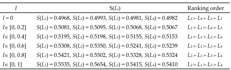
Table 6. Ranking order with variation of “I”on NNsfor strategy 2

329

I S(Li) Ranking order

I = 0 S(L1) = 0.4968, S(L2) = 0.4993, S(L3) = 0.4981, S(L4) = 0.4982 L2L4L3L1 I∈[0, 0.2] S(L1) = 0.5081, S(L2) = 0.5095, S(L3) = 0.5068, S(L4) = 0.5067 L2L1L4L3 I∈[0, 0.4] S(L1) = 0.5195, S(L2) = 0.5198, S(L3) = 0.5155, S(L4) = 0.5153 L2L1L3L4 I∈[0, 0.6] S(L1) = 0.5308, S(L2) = 0.5350, S(L3) = 0.5241, S(L4) = 0.5239 L2L1L3L4 I∈[0, 0.8] S(L1) = 0.5421, S(L2) = 0.5502, S(L3) = 0.5328, S(L4) = 0.5324 L2L1L3L4 I∈[0, 1] S(L1) = 0.5535, S(L2) = 0.5654, S(L3) = 0.5415, S(L4) = 0.5410 L2L1L3L4

Step 6. Food company (FOODC)is the best alternative for investment.

330

Step 7. End

331

332

333

334

335

336

337

7. Comparison analysis and contributions of the proposed approach

338

7.1. Comparison analysis

339

In this subsection, a comparison analysis is conducted between the proposed MCGDM strategies

340

and other existing strategies in NN environment. Table 5 reflects that L2 is the best alternative for I = 0

341

andI≠0. Table 6 reflects that L2 is the best alternative for any values of I. The ranking results

342

obtained from the existing strategies [12, 13, 17] are furnished in Table 7.

343

In strategy [17], deneutrosophication process is analyzed. It does not recognize the importance of

344

the aggregation information. MCGDM due to Liu and Liu [12] is based on NN generalized weighted

345

power averaging operator. This strategy cannot deal the situation when larger value other than

346

arithmetic mean, geometric mean and harmonic mean is necessary for experiment purpose. In Zheng

347

et al. [13], the NN general hybrid weighted averaging operators are proposed. The strategy proposed

348

0.46 0.48 0.5 0.52 0.54 0.56 0.58

CARC FOODC COMC ARMC

I = [0, 0]

I = [0, 0.2]

I = [0, 0.4]

I = [0, 0.6]

I = [0, 0.8]

I = [0, 1]

(13)

by Zheng et al. [13] cannot be used when few observations contribute disproportionate amount to the

349

arithmetic mean. To overcome the problem, we have proposed two NN harmonic aggregation

350

operators for MCGDM.

351

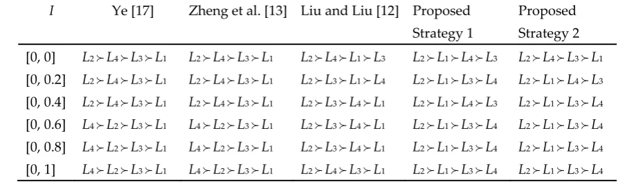
Table 7. Comparison of ranking results with variation of ‘I’ on NNs for different strategies

352

I Ye [17] Zheng et al. [13] Liu and Liu [12] Proposed

Strategy 1

Proposed Strategy 2 [0, 0] L2L4L3L1 L2L4L3L1 L2L4L1L3 L2L1L4L3 L2L4L3L1

[0, 0.2] L2L4L3L1 L2L4L3L1 L2L3L1L4 L2L1L3L4 L2L1L4L3

[0, 1] L4L2L3L1 L4L2L3L1 L2L4L3L1 L2L1L3L4 L2L1L3L4

353

7.2. Contributions of the proposed approach

354

• NNHMO and NNWHMO in NN environment are firstly defined in the literature. We also

355

proved their basic properties.

356

• We proposed score and accuracy functions of NN numbers. If two score values are same,

357

then accuracy function can be used for ranking purpose.

358

• The proposed two strategies can also used when observations/experiments contribute is

359

disproportionate amount to the arithmetic mean. The harmonic mean is used when sample

360

values contain fractions and/or extreme values (either too small or too big).

361

• To calculate unknown weights structure in NN environment, cosine function is proposed.

362

• Steps and calculations of the proposed strategies are easy to use.

363

• We have solved a numerical example to show the feasibility, applicability, and effectiveness

364

of the proposed two strategies.

365

8. Conclusions

366

In the study, we have proposed NNHMO and NNWHMO. We have developed two strategies of

367

ranking NNs based on proposed score function and accuracy function. We have proposed cosine

368

function to determine unknown criteria weights in NN environment. We have developed two novel

369

MCGDM strategies based on the proposed aggregation operators. We have solved a hypothetical

370

case study and compared the obtained results with other existing strategies to demonstrate the

371

effectiveness of the proposed MCGDM strategies. Sensitivity analysis for different values of I is also

372

conducted to show the influence of I in preference ranking of the alternatives. The significance of the

373

paper is that we combine NNs with harmonic aggregation operators to cope with MCGDM

374

problems. We hope that the proposed two MCGDM strategies will open up new avenue of research

375

in NN environment for dealing with MCGDM problems and its practical implementation to real

376

world decision making problems in the current neutrosophic decision making arena.

377

Author Contributions: Kalyan Mondal and Surapati Pramanik conceived and designed the experiments;

378

Kalyan Mondal, and Surapati Pramanik performed the experiments; Surapati Pramanik and B. C. Giri

379

analyzed the data; Kalyan Mondal, Surapati Pramanik, and B. C. Giri contributed to analysis tools; Kalyan

380

Mondal and Surapati Pramanik wrote the paper.

(14)

Conflicts of Interest: The authors declare no conflict of interest.

382

References

383

1. Ma, Y.X.; Wang, J.Q.; Wang, J.; Wu, X.H. An interval neutrosophic linguistic multi-criteria group

384

decision-making method and its application in selecting medical treatment options. Neural. Comput. Appl.

385

2017, 28, 2745–2765.

386

2. Liu, H.C.; Wu, J.; Li, P. Assessment of health-care waste disposal methods using a VIKOR-based fuzzy

387

multi-criteria decision making method. Waste. Manag. 2013, 33, 2744–2751.

388

3. Tian, Z.P.; Wang, J.; Wang, J.Q.; Zhang, H.Y. Simplified neutrosophic linguistic multi-criteria group

389

decision-making approach to green product development. Group. Decis. Negot. 2017, 26, 597–627.

390

4. Biswas, P.; Pramanik, S.; Giri, B.C. TOPSIS method for multi-attribute group decision-making under

391

single-valued neutrosophic environment. Neural. Comput. Appl. 2016, 27, 727–737.

392

5. Zouggari, A.; Benyoucef, L. Simulation based fuzzy TOPSIS approach for group multi-criteria supplier

393

selection problem. Eng. Appl. Artif. Intell. 2012, 25, 507–519.

394

6. Smarandache, F. Introduction to neutrosophic measure, neutrosophic integral, and neutrosophic.

395

Probability, Sitech & Education Publisher, Craiova, 2013.

396

7. Smarandache, F. Introduction to neutrosophic statistics. Sitech & Education Publishing, Columbus, 2014.

397

8. Park, J.H.; Gwak, M.G.; Kwun, Y.C. Uncertain linguistic harmonic mean operators and their applications to

398

multiple attribute group decision making. Computing. 2011, 93, 47–64.

399

9. Wei, G.W. FIOWHM operator and its application to multiple attribute group decision making. Expert. Syst.

400

Appl. 2011, 38, 2984–2989.

401

10. Xu, Z. Fuzzy harmonic mean operators. Int. J. Intell. Syst. 2009, 24, 152–172.

402

11.Ye, J. Simplified neutrosophic harmonic averaging projection-based strategy for multiple attribute

403

decision-making problems. Int. J. Mach. Learn. Cybern. 2017, 8, 981–987.

404

12. Liu, P.; Liu, X. The neutrosophic number generalized weighted power averaging operator and its

405

application in multiple attribute group decision making. Int J Mach Learn Cybernet. 2016, 1–12.

406

https://doi.org/10.1007/s13042-016-0508-0

407

13. Zheng, E.; Teng, F.; Liu, P. Multiple attribute group decision-making strategy based on neutrosophic

408

number generalized hybrid weighted averaging operator. Neural .Comput. Appl. 2017, 28, 2063–2074.

409

14.Pramanik S.; Roy R.; Roy T.K. Teacher selection strategy based on bidirectional projection measure in

410

neutrosophic number environment. In Neutrosophic Operational Research; Smarandache, F., Abdel-Basset, M.,

411

El-Henawy, I., Eds.; Pons Publishing House / Pons asbl: Bruxelles, Belgium, 2017; Volume 2, ISBN

412

978-1-59973-537-5. (In Press).

413

15. Majumdar, P.; Samanta, S.K. On similarity and entropy of neutrosophic sets. J. Intell. Fuzzy. Syst. 2014, 26,

414

1245–1252.

415

16.Biswas, P.; Pramanik, S.; Giri, B.C. Entropy based grey relational analysis strategy for multi-attribute

416

decision-making under single valued neutrosophic assessments. Neutrosophic. Sets. Syst. 2014, 2,102–110.

417

17. Ye, J. Multiple attribute group decision making method under neutrosophic number environment. J. Intell.

418

Syst. 2016, 25, 377–386.