Logistic Regression Model Training based on the
Approximate Homomorphic Encryption
Andrey Kim1, Yongsoo Song2?, Miran Kim2, Keewoo Lee1, and Jung Hee Cheon1
1
Seoul National University, Seoul, Republic of Korea
{kimandrik, activecondor, jhcheon}@snu.ac.kr
2
University of California, San Diego, United States
{yongsoosong, mrkim}@ucsd.edu
Abstract. Security concerns have been raised since big data became a prominent tool in data analysis. For instance, many machine learning algorithms aim to generate prediction models using training data which contain sensitive information about individuals. Cryptography com-munity is considering secure computation as a solution for privacy protection. In particular, practical requirements have triggered research on the efficiency of cryptographic primitives. This paper presents a practical method to train a logistic regression model while preserving the data confidentiality We apply the homomorphic encryption scheme of Cheon et al. (ASI-ACRYPT 2017) for an efficient arithmetic over real numbers, and devise a new encoding method to reduce storage of encrypted database. In addition, we adapt Nesterov’s accelerated gradient method to reduce the number of iterations as well as the computational cost while maintaining the quality of an output classifier.
Our method shows a state-of-the-art performance of homomorphic encryption system in a real-world application. The submission based on this work was selected as the best solution of Track 3 at iDASH privacy and security competition 2017. For example, it took about six minutes to obtain a logistic regression model given the dataset consisting of 1579 samples, each of which has 18 features with a binary outcome variable.
Keywords.Homomorphic encryption, machine learning, logistic regression
1 Background
Machine learning (ML) is a class of methods in artificial intelligence, the characteristic feature of which is that they do not give the solution of a particular problem but they learn the process of finding solutions to a set of similar problems. The theory of ML appeared in the early 60’s on the basis of the achievements of cybernetics [25] and gave the impetus to the development of theory and practice of technically complex learning systems [7]. The goal of ML is to partially or fully automate the solution of complicated tasks in various fields of human activity.
The scope of ML applications is constantly expanding; however, with the rise of ML, the security problem has become an important issue. For example, many medical decisions rely on logistic regression model, and biomedical data usually contain confidential information about individuals [24] which should be treated carefully. Therefore, privacy and security of data are the major concerns, especially when deploying the outsource analysis tools.
There have been several researches on secure computation based on cryptographic prim-itives. Nikolaenko et al. [20] presented a privacy preserving linear regression protocol on horizontally partitioned data using Yao’s garbled circuits [30]. Multi-party computation tech-nique was also applied to privacy-preserving logistic regression [8, 17, 16]. However, this ap-proach is vulnerable when a party behaves dishonestly, and the assumption for secret sharing is quite different from that of outsourcing computation.
techniques. Wu et al. [28] used Paillier cryptosystem [21] and approximated the logistic func-tion using polynomials, but it required an exponentially growing computafunc-tional cost in the degree of the approximation polynomial. Aono et al. [2] and Xie et al. [29] used an additive HE scheme to aggregate some intermediate statistics. However, the scenario of Aono et al. relies on the client to decrypt these intermediary statistics and the method of Xie et al. requires expensive computational cost to calculate the intermediate information. The most related research of this paper is the work of Kim et al. [12] which also used HE based ML. However, the size of encrypted data and learning time were highly dependent on the number of features, so the performance for a large dataset was not practical in terms of storage and computational cost.
Since 2011, the iDASH Privacy and Security Workshop has assembled specialists in pri-vacy technology to discuss issues that apply to biomedical data sharing, as well as main stakeholders who provided an overview of the main uses of the data, different laws and regu-lations, and their own views on privacy. In addition, it has began to hold annual competitions on the basis of the workshop from 2014. The goal of this challenge is to evaluate the per-formance of state-of-the-arts methods that ensures rigorous data confidentiality during data analysis in a cloud environment.
In this paper, we provide a solution to the third track of iDASH 2017 competition, which aims to develop HE based secure solutions for building a ML model (i.e., logistic regression) over encrypted data. We propose a general practical solution for HE based ML that demonstrates good performance and low storage costs. In practice, our output quality is comparable to the one of an unencrypted learning case. As a basis, we use the HE scheme for approximate arithmetic [6]. To improve the performance, we apply several additional techniques including a packing method, which reduce the required storage space and optimize the computational time. We also adapt Nesterov’s accelerated gradient [18] to improve the convergence rate. As a result, we used less number of iterations than the other solutions, resulting in a much faster time to learn a model.
We give an open-source implementation [4] to demonstrate the performance of our HE based ML method. With our packing method we can encrypt the dataset with 1579 samples and 18 features using 39MB of memory. The encrypted learning time is about six minutes. We also demonstrate our implementation on the datasets used in [12] to compare the results. For example, the training of a logistic regression model took about 3.6 minutes with the storage about 0.02GB compared to 114 minutes and 0.69GB of Kim et al. [12] when a dataset consists of 1253 samples, each of which has 9 features.
2 Methods
2.1 Logistic Regression
Logistic regression or logit model is a ML model used to predict the probability of occurrence of an event by fitting data to a logistic curve [10]. It is widely used in various fields including machine learning, biomedicine [15], genetics [14], and social sciences [9].
Throughout this paper, we treat the case of a binary dependent variable, represented by
±1. Learning data consists of pairs (xi, yi) of a vector of co-variatesxi = (xi1, ..., xif)∈Rf and a dependent variable yi ∈ {±1}. Logistic regression aims to find an optimal β∈ Rf+1 which maximizes the likelihood estimator
n Y
i=1
Pr(yi|xi) = n Y
i=1
1
1 + exp(−yi(1,xi)Tβ)
or equivalently minimizes the loss function, defined as the negative log-likelihood:
J(β) = 1
n
n X
i=1
log(1 + exp(−zTi β))
wherezi =yi·(1,xi) for i= 1, . . . , n.
2.2 Gradient Descent
Gradient Descent (GD) is a method for finding a local extremum (minimum or maximum) of a function by moving along gradients. To minimize the function in the direction of the gradient, one-dimensional optimization methods are used.
For logistic regression, the gradient of the cost function with respect to β is computed by
∇J(β) =−1
n
n X
i=1
σ(−zTi β)·zi
where σ(x) = 1+exp(1 −x). Starting from an initial β0, the gradient descent method at each stept updates the regression parameters using the equation
β(t+1)←β(t)+αt
n
n X
i=1
σ(−zTi β(t))·zi
whereαtis a learning rate at step t.
2.3 Nesterov’s Accelerated Gradient
The method of GD can face a problem of zig-zagging along a local optima and this behavior of the method becomes typical if it increases the number of variables of an objective function. Many GD optimization algorithms are widely used to overcome this phenomenon. Momentum method, for example, dampens oscillation using the accumulated exponential moving average for the gradient of the loss function.
Nesterov’s accelerated gradient [18] is a slightly different variant of the momentum up-date. It uses moving average on the update vector and evaluates the gradient at this “looked-ahead” position. It guarantees a better rate of convergence O(1/t2) (vs. O(1/t) of standard GD algorithm) after tsteps theoretically, and consistently works slightly better in practice. Starting with a random initial v0 =β0, the updated equations for Nesterov’s Accelerated GD are as follows:
(
β(t+1) =v(t)−αt· 5J(v(t)), v(t+1) = (1−γt)·β(t+1)+γt·β(t),
(1)
where 0< γt<1 is a moving average smoothing parameter.
2.4 Approximate Homomorphic Encryption
The following is a simple description of HEAAN based on the ring learning with errors problem. For a power-of-two integer N, the cyclotomic polynomial ring of dimension N
is denoted by R = Z[X]/(XN + 1). For a positive integer `, we denote R` = R/2`R =
Z2`[X]/(XN+ 1) the residue ring of Rmodulo 2`.
• KeyGen(1λ).
- For an integer L that corresponds to the largest ciphertext modulus level, given the security parameterλ, output the ring dimension N which is a power of two.
- Set the small distributions χkey, χerr, χenc over R for secret, error, and encryption,
respectively.
- Sample a secrets←χkey, a randoma← RLand an errore←χerr. Set the secret key
assk←(1, s) and the public key aspk←(b, a)∈ R2
L whereb← −as+e (mod 2L). • KSGensk(s0). For s0 ∈ R, sample a random a0 ← R2·L and an errore0 ←χerr. Output the
switching key asswk←(b0, a0)∈ R2
2·L whereb
0 ← −a0s+e0+ 2Ls0 (mod 22·L).
- Set the evaluation key asevk←KSGensk(s2).
• Encpk(m). For m ∈ R, samplev ← χenc and e0, e1 ← χerr. Output v·pk+ (m+e0, e1) (mod 2L).
• Decsk(ct). For ct= (c0, c1)∈ R`2, output c0+c1·s (mod 2`).
• Add(ct1,ct2). For ct1,ct2∈ R2
`, outputctadd←ct1+ct2 (mod 2`). • CMultevk(ct;c). Forct∈ R2` and a∈ R, output ct
0 ←c·ct (mod 2`).
• Multevk(ct1,ct2). For ct1 = (b1, a1),ct2 = (b2, a2) ∈ R2`, let (d0, d1, d2) = (b1b2, a1b2+
a2b1, a1a2) (mod 2`). Outputctmult←(d0, d1) +b2−L·d2·evke (mod 2`).
• ReScale(ct;p). For a ciphertext ct ∈ R2
` and an integer p, output ct
0 ← b2−p·cte
(mod 2`−p).
For a power-of-two integer k ≤ N/2, HEAAN provides a technique to pack k complex numbers in a single polynomial using a variant of the complex canonical embedding map
φ : Ck → R. We restrict the plaintext space as a vector of real numbers throughout this paper. Moreover, we multiply a scale factor of 2p to plaintexts before the rounding operation to maintain their precision.
• Encode(w;p). For w∈Rk, output the polynomialm←φ(2p·w)∈ R.
• Decode(m;p). For a plaintext m∈ R, the encoding of an array consisting of a power of two k≤N/2 messages, output the vectorw←φ−1(m/2p)∈Rk.
The encoding/decoding techniques support the parallel computation over encryption, yielding a better amortized timing. In addition, theHEAANscheme provides the rotation op-eration on plaintext slots, i.e., it enables us to securely obtain an encryption of the shifted plaintext vector (wr, . . . , wk−1, w0, . . . , wr−1) from an encryption of (w0, . . . , wk−1). It is nec-essary to generate an additional public information rk, called the rotation key. We denote the rotation operation as follows.
• Rotaterk(ct;r). For the rotation keysrk, output a ciphertext ct0 encrypting the rotated
plaintext vector of ct byr positions.
2.5 Database Encoding
For an efficient computation, it is crucial to find a good encoding method for the given database. The HEAAN scheme supports the encryption of a plaintext vector and the slot-wise operations over encryption. However, our learning data is represented by a matrix (zij)1≤i≤n,0≤j≤f. A recent work [12] used the column-wise approach, i.e., a vector of specific
feature data (zij)1≤i≤nis encrypted in a single ciphertext. Consequently, this method required
(f + 1) number of ciphertexts to encrypt the whole dataset.
In this subsection, we suggest a more efficient encoding method to encrypt a matrix in a single ciphertext. A training dataset consists ofn sampleszi ∈Rf+1 for 1≤i≤n, which can be represented as a matrixZ as follows:
Z =
z10 z11· · ·z1f
z20 z21· · ·z1f
..
. ... . .. ...
zn0 zn1· · ·znf
.
For simplicity, we assume that n and (f + 1) are power-of-two integers satisfying logn+ log(f + 1)≤log(N/2). Then we can pack the whole matrix in a single ciphertext in a row-by-row manner. Specifically, we will identify this matrix with the k-dimensional vector by (zij)1≤i≤n,0≤j≤f 7→ w = (w`)0≤`<n·(f+1) where w` = zij such that ` = (f+ 1)(i−1) +j,
that is,
Z7→w= (z10, . . . , z1f, z20, . . . , z2f, . . . , zn0, . . . , znf).
In a general case, we can pad zeros to set the number of samples and the dimension of a weight vector as powers of two.
It is necessary to perform shifting operations of row and column vectors for the evalu-ation of the GD algorithm. In the rest of this subsection, we explain how to perform these operations using the rotation algorithm provided in the HEAANscheme. As described above, the algorithmRotate(ct;r) can shift the encrypted vector by r positions. In particular, this operation is useful in our implementation whenr=f+ 1 orr = 1. For the first case, a given matrixZ = (zij)1≤i≤n,0≤j≤f is converted into the matrix
Z0 =
z20 z21· · ·z2f
..
. ... . .. ...
zn0 zn1· · ·znf
z10 z11· · ·z1f
,
while the latter case outputs the matrix
Z00=
z11 · · ·z1f z20
z21 · · ·z2f z30 ..
. ... . .. ...
zn1 · · ·znf z10
over encryption. The matrix Z0 is obtained from Z by shifting its row vectors and Z00 can be viewed as an incomplete column shifting because of its last column.
2.6 Polynomial Approximation of the Sigmoid Function
Kim et al. [12] used the least squares approach to find a global polynomial approximation of the sigmoid function. We adapt this approximation method and consider the degree 3, 5, and 7 least squares polynomials of the sigmoid function over the domain [−8,8]. We observed that the inner product values zTi β(t) in our experimentations belong to this interval. For simplicity, a least squares polynomial of σ(−x) will be denoted by g(x) so that we have
g(zTi β(t)) ≈σ(−zTi β(t)) when |zTiβ(t)| ≤8. The approximate polynomials g(x) of degree 3, 5, and 7 are computed as follows:
g3(x) = 0.5−1.20096·(x/8) + 0.81562·(x/8)3,
g5(x) = 0.5−1.53048·(x/8) + 2.3533056·(x/8)3−1.3511295·(x/8)5,
g7(x) = 0.5−1.73496·(x/8) + 4.19407·(x/8)3−5.43402·(x/8)5+ 2.50739·(x/8)7.
A low-degree polynomial requires a smaller evaluation depth while a high-degree polynomial has a better precision. The maximum errors between σ(−x) and the least squares g3(x),
g5(x), and g7(x) are approximately 0.114, 0.061 and 0.032, respectively.
2.7 Homomorphic Evaluation of the Gradient Descent
This section explains how to securely train the logistic regression model using the HEAAN
scheme. To be precise, we explicitly describe a full pipeline of the evaluation of the GD algorithm. We adapt the same assumptions as in the previous section so that the whole database can be encrypted in a single ciphertext.
First of all, a client encrypts the dataset and the initial (random) weight vectorβ(0) and sends them to the public cloud. The dataset is encoded to a matrixZ of sizen×(f+ 1) and the weight vector is copied ntimes to fill the plaintext slots. The plaintext matrices of the resulting ciphertexts are described as follows:
ctz =Enc
z10 z11· · ·z1f
z20 z21· · ·z1f
..
. ... . .. ...
zn0zn1· · ·znf
, ct(0)β =Enc
β0(0)β1(0)· · ·βf(0) β0(0)β1(0)· · ·βf(0)
..
. ... . .. ...
β0(0)β1(0)· · ·βf(0)
.
As mentioned before, both Z and β(0) are scaled by a factor of 2p before encryption to maintain the precision of plaintexts. We skip to mention the scaling factor in the rest of this section since every step will return a ciphertext with the scaling factor of 2p.
The public server takes two ciphertexts ctz andct(βt) and evaluates the GD algorithm to
find an optimal modeling vector. The goal of each iteration is to update the modeling vector
β(t) using the gradient of loss function:
β(t+1)←β(t)+αt
n
n X
i=1
σ(−zTi β(t))·zi
whereαtdenotes the learning rate at thet-th iteration. Each iteration consists of the following
eight steps.
Step 1:For given two ciphertexts ctz and ct(βt), compute their multiplication and rescale it
by pbits:
The output ciphertext contains the valueszij·β
(t)
j in its plaintext slots, i.e.,
ct1 =Enc
z10·β (t) 0 z11·β
(t)
1 · · · z1f·β
(t)
f
z20·β(0t) z21·β1(t) · · · z1f·βf(t)
..
. ... . .. ...
zn0·β0(t) zn1·β1(t) · · · znf ·βf(t) .
Step 2:To obtain the inner productzTi β(t), the public cloud aggregates the values ofzijβj(t)
in the same row. This step can be done by adapting the incomplete column shifting operation. One simple way is to repeat this operation (f+ 1) times, but the computational cost can be reduced down to log(f+ 1) by adding ct1 to its rotations recursively:
ct1 ←Add(ct1,Rotate(ct1; 2j)),
for j = 0,1, . . . ,log(f + 1)−1. Then the output ciphertext ct2 encrypts the inner product values zTi β(t) in the first column and some “garbage” values in the other columns, denoted by ?, i.e.,
ct2=Enc
zT1β(t) ? · · · ?
zT2β(t) ? · · · ?
..
. ... . .. ...
zTnβ(t) ? · · · ?
.
Step 3: This step performs a constant multiplication in order to annihilate the garbage values. It can be obtained by computing the encoding polynomialc←Encode(C;pc) of the
matrix C=
1 0 · · · 0 1 0 · · · 0
..
. ... . .. ... 1 0 · · · 0
,
using the scaling factor of 2pc for some integer p
c. The parameter pc is chosen as the bit
precision of plaintexts so it can be smaller than the parameterp.
Finally we multiply the polynomial c to the ciphertextct2 and rescale it by pc bits:
ct3 ←ReScale(CMult(ct2;c);pc).
The garbage values are multiplied with zero while one can maintain the inner products in the plaintext slots. Hence the output ciphertextct3 encrypts the inner product values in the first column and zeros in the others:
ct3=Enc
zT1β(t) 0 · · · 0
zT2β(t) 0 · · · 0 ..
. ... . .. ...
zTnβ(t) 0 · · · 0
.
Step 4:The goal of this step is to replicate the inner product values to other columns. Similar to Step 2, it can be done by adding the input ciphertext to its column shifting recursively, but in the opposite direction
forj= 0,1, . . . ,log(f + 1)−1. The output ciphertextct4 has the same inner product value in each row:
ct4 =Enc
zT1β(t) zT1β(t) · · · zT1β(t) zT2β(t) zT2β(t) · · · zT2β(t)
..
. ... . .. ...
zT
nβ(t) zTnβ(t) · · · zTnβ(t) .
Step 5: This step simply evaluates an approximating polynomial of the sigmoid function, i.e., ct5 ← g(ct4) for some g ∈ {g3, g5, g7}. The output ciphertext encrypts the values of
g(zT
i β(t)) in its plaintext slots:
ct5 =Enc
g(zT1β(t)) · · · g(zT1β(t))
g(zT
2β(t)) · · · g(zT2β(t)) ..
. . .. ...
g(zTnβ(t)) · · · g(zTnβ(t))
.
Step 6: The public cloud multiplies the ciphertext ct5 with the encrypted dataset ctz and
rescales the resulting ciphertext byp bits:
ct6←ReScale(Mult(ct5,ctz);p).
The output ciphertext encrypts thenvectors g(zTi β(t))·zi in each row:
ct6=Enc
g(zT1β(t))·z10 · · · g(zT1β(t))·z1f
g(zT2β(t))·z20 · · · g(zT2β(t))·z2f
..
. . .. ...
g(zT
nβ(t))·zn0 · · · g(zTnβ(t))·znf .
Step 7: This step aggregates the vectors g(zTi β(t)) to compute the gradient of the loss function. It is obtained by recursively addingct6 to its row shifting:
ct6 ←Add(ct6,Rotate(ct6; 2j))
forj= log(f+ 1), . . . ,log(f+ 1) + logn−1. The output ciphertext is
ct7 =Enc
P
ig(zTi β(t))·zi0 · · · Pig(zTi β(t))·zif P
ig(zTi β(t))·zi0 · · · Pig(zTi β(t))·zif
..
. . .. ...
P
ig(zTi β(t))·zi0 · · · Pig(zTi β(t))·zif , as desired.
Step 8:For the learning rateαt, it uses the parameterpcto compute the scaled learning rate
∆(t) = b2pc·α
te. The public cloud updates β(t) using the ciphertext ct7 and the constant
∆(t):
ct8←ReScale(∆(t)·ct7;pc),
ctβ(t+1) ←Add(ctβ(t),ct8).
Finally it returns a ciphertext encrypting the updated modeling vector
ct(βt+1) =Enc
β0(t+1) β1(t+1) · · · βf(t+1) β0(t+1) β1(t+1) · · · βf(t+1)
..
. ... . .. ...
β0(t+1) β1(t+1) · · · βf(t+1)
.
whereβj(t+1)=βj(t)+ αt
n P
2.8 Homomorphic Evaluation of Nesterov’s Accelerated Gradient
The performance of leveled HE schemes highly depends on the depth of a circuit to be evaluated. The bottleneck of homomorphic evaluation of the GD algorithm is that we need to repeat the update of weight vector β(t) iteratively. Consequently, the total depth grows linearly on the number of iterations and it should be minimized for practical implementation. For the homomorphic evaluation of Nesterov’s accelerated gradient, a clients sends one more ciphertextct(0)v encrypting the initial vector v(0) to the public cloud. Then the server
uses an encryptionctzof datasetZ to update two ciphertextsv(t)andct(βt)at each iteration.
One can securely computeβ(t+1) in the same way as the previous section. Nesterov’s accel-erated gradient requires one more step to compute the second equation of (1) and obtain an encryption ofv(t+1) from ctβ(t) and ct(βt+1).
Step 9: Let ∆(1t) = b2pc ·γ
te and let∆(2t) = 2pc −∆ (t)
1 . It obtains the ciphertext ct (t+1)
v by
computing
ctv(t+1)←Add(∆(2t)·ctβ(t+1), ∆(1t)·ct(βt)),
ctv(t+1)←ReScale(ctv(t+1);pc).
Then the output ciphertext is
ct(vt+1)=Enc
v(0t+1) v(1t+1) · · · v(ft+1) v(0t+1) v(1t+1) · · · v(ft+1)
..
. ... . .. ...
v(0t+1) v(1t+1) · · · v(ft+1)
,
which encrypts v(jt+1)= (1−γt)·βj(t+1)+γt·βj(t) in the plaintext slots.
3 Results
In this section, we present parameter sets with experimental results. Our implementation is based on the HEAAN library [5] that implements the HE scheme of Cheon et al. [6]. The source code is publicly available at github[4].
3.1 Parameters settings
We explain how to choose the parameter sets for the homomorphic evaluation of the (Nes-terov’s) GD algorithm with security analysis. We start with the parameter L - the bitsize of a fresh ciphertext modulus. The modulus of a ciphertext is reduced after the ReScale
operations and the evaluation of an approximate polynomial g(x).
The ReScale procedures after homomorphic multiplications (step 1 and 6) reduce the ciphertext modulus by p bits while the ReScale procedures after constant multiplications (step 3 and 8) requirepcbits of modulus reduction. Note that the ciphertext modulus remains
the same for the step 9 for the Nesterov’s accelerated gradient if we compute step 8 and 9 together using some precomputed constants. We use a similar method with a previous work for the evaluation of the sigmoid function (see [12] for details); the ciphertext modulus is reduced by (2p+ 3) bits for the evaluation ofg3(x), and (3p+ 3) bits for that of g5(x) and
g7(x). Therefore, we obtain the following lower bound on the parameter L:
L=
(
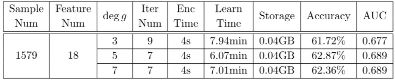
Table 1.Implementation results for iDASH dataset with 10-fold CV
Sample Feature
degg Iter Enc Learn Storage Accuracy AUC
Num Num Num Time Time
1579 18
3 9 4s 7.94min 0.04GB 61.72% 0.677
5 7 4s 6.07min 0.04GB 62.87% 0.689
7 7 4s 7.01min 0.04GB 62.36% 0.689
whereIterNumis the number of iterations of the GD algorithm andL0 denotes the bit size of the output ciphertext modulus. The modulus of the output ciphertext should be larger than 2p in order to encrypt the resulting weight vector and maintain its precision. We take
p= 30,pc= 20 and L0 = 35 in our implementation.
The dimension of a cyclotomic ring R is chosen as N = 216 following the security esti-mator of Albrecht et al. [1] for the learning with errors problem. In this case, the bit sizeL
of a fresh ciphertext modulus should be bounded by 1284 to ensure the security levelλ= 80 against known attacks. Hence we repeat IterNum= 9 iterations of GD algorithm g= g3, and IterNum= 7 iterations when g=g5 org=g7.
The smoothing parameterγt is chosen in accordance with [18]. The choice of proper GD
learning rate parameter αt normally depends on the problem at hand. Choosing too small
αt leads to a slow convergence, and choosing too large αt could lead to a divergence, or a
fluctuation near a local optima. It is often optimized by a trial and error method, which we are not available to perform. Under these conditions harmonic progression seems to be a good candidate and we choose a learning rateαt= t10+1 in our implementation.
3.2 Implementation
All the experimentations were performed on a machine with an Intel Xeon CPU E5-2620 v4 at 2.10 GHz processor.
Task for iDASH challenge. In genomic data privacy and security protection competition
2017, the goal of Track 3 was to devise a weight vector to predict the disease using the genotype and phenotype data. This dataset consists of 1579 samples, each of which has 18 features and a cohort information (disease vs. healthy). Since we use the ring dimension
N = 216, we can only pack up to N/2 = 215 dataset values in a single ciphertext but we have totally 1579×19 > 215 values to be packed. We can overcome this issue by dividing the dataset into two parts of sizes 1579×16 and 1579×3 and encoding them separately into two ciphertexts. In general, this method can be applied to the datasets with any number of features: the dataset can be encrypted as d(f + 1)·n·(N/2)−1eciphertexts.
In order to estimate the validity of our method, we utilized 10-fold cross-validation (CV) technique: it randomly partitions the dataset into ten folds with approximately equal sizes, and uses every subset of 9 folds for training and the rest one for testing the model. The performance of our solution including the average running time (encryption and evaluation) and the storage (encrypted dataset) are shown in Table 1. This table also provides the average accuracy and the AUC (Area Under the Receiver Operating Characteristic Curve) which estimate the quality of a binary classifier.
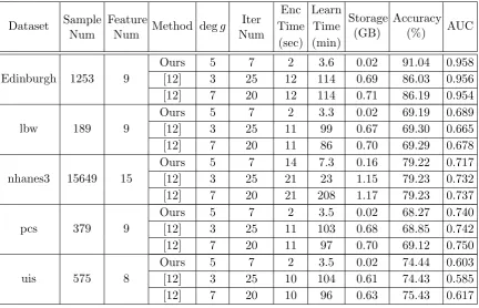
Comparison. We present some experimental results to compare the performance of
Table 2.Implementation results for other datasets with 5-fold CV
Dataset Sample Num
Feature
Num Method degg Iter Num
Enc Learn
Storage (GB)
Accuracy
(%) AUC
Time Time (sec) (min)
Edinburgh 1253 9
Ours 5 7 2 3.6 0.02 91.04 0.958
[12] 3 25 12 114 0.69 86.03 0.956
[12] 7 20 12 114 0.71 86.19 0.954
lbw 189 9
Ours 5 7 2 3.3 0.02 69.19 0.689
[12] 3 25 11 99 0.67 69.30 0.665
[12] 7 20 11 86 0.70 69.29 0.678
nhanes3 15649 15
Ours 5 7 14 7.3 0.16 79.22 0.717
[12] 3 25 21 23 1.15 79.23 0.732
[12] 7 20 21 208 1.17 79.23 0.737
pcs 379 9
Ours 5 7 2 3.5 0.02 68.27 0.740
[12] 3 25 11 103 0.68 68.85 0.742
[12] 7 20 11 97 0.70 69.12 0.750
uis 575 8
Ours 5 7 2 3.5 0.02 74.44 0.603
[12] 3 25 10 104 0.61 74.43 0.585
[12] 7 20 10 96 0.63 75.43 0.617
Weight Study (lbw), Nhanes III (nhanes3), Prostate Cancer Study (pcs), and Umaru Impact Study datasets (uis) [13, 19, 22, 26]. All datasets have a single binary outcome variable.
All the experimental results are summarized in Table 2. Our new packing method could reduce the storage of ciphertexts and the use of Nesterov’s accelerated gradient achieves much higher speed than the approach of [12]. For example, it took 3.6 minutes to train a logistic regression model using the encrypted Edinburgh dataset of size 0.02 GB, compared to 114 minutes and 0.69 GB of the previous work, while keeping the good qualities of the output models.
4 Discussion
The rapid growth of computing power initiated the study of more complicated ML algorithms in various fields including biomedical data analysis [27, 23]. HE system is a promising solution for the privacy issue, but its efficiency in real applications remains as an open question. It would be great if we could extend this work to other ML algorithms such as deep learning.
One constraint in our approach is that the number of iterations of GD algorithm is limited depending on the choice of HE parameter. In terms of asymptotic complexity, applying the bootstrapping method of approximate HE scheme [3] to the GD algorithm would achieve a linear computation cost on the iteration number.
5 Conclusion
A Abbreviations
ML: Machine Learning; HE: Homomorphic Encryption; GD: Gradient Descent; CV: Cross Validation; AUC: Area Under the receiver operating characteristic Curve
B Availability of data and material
All datasets are available in the Additional files provided with the publication. The HEAAN
library is available at https://github.com/kimandrik/HEAAN. Our implementation is avail-able at https://github.com/kimandrik/HEML.
References
1. M. R. Albrecht, R. Player, and S. Scott. On the concrete hardness of learning with errors. Journal of Mathematical Cryptology, 9(3):169–203, 2015.
2. Y. Aono, T. Hayashi, L. Trieu Phong, and L. Wang. Scalable and secure logistic regression via homo-morphic encryption. InProceedings of the Sixth ACM Conference on Data and Application Security and Privacy, pages 142–144. ACM, 2016.
3. J. H. Cheon, K. Han, A. Kim, M. Kim, and Y. Song. Bootstrapping for approximate homomorphic encryption. Cryptology ePrint Archive, Report 2018/153, 2018. https://eprint.iacr.org/2018/153. 4. J. H. Cheon, A. Kim, M. Kim, K. Lee, and Y. Song. Implementation for idash competition 2017, 2017.
https://github.com/kimandrik/HEML.
5. J. H. Cheon, A. Kim, M. Kim, and Y. Song. Implementation of HEAAN, 2016. https://github.com/kimandrik/HEAAN.
6. J. H. Cheon, A. Kim, M. Kim, and Y. Song. Homomorphic encryption for arithmetic of approximate numbers. InAdvances in Cryptology–ASIACRYPT 2017: 23rd International Conference on the Theory and Application of Cryptology and Information Security, pages 409–437. Springer, 2017.
7. E. Dietz. Application of logistic regression and logistic discrimination in medical decision making. Bio-metrical journal, 29(6):747–751, 1987.
8. K. El Emam, S. Samet, L. Arbuckle, R. Tamblyn, C. Earle, and M. Kantarcioglu. A secure distributed logistic regression protocol for the detection of rare adverse drug events.Journal of the American Medical Informatics Association, 20(3):453–461, 2012.
9. V. Gayle and P. S. Lambert. Logistic regression models in sociological research. 2009.
10. F. E. Harrell. Ordinal logistic regression. InRegression modeling strategies, pages 331–343. Springer, 2001.
11. R. Kennedy, H. Fraser, L. McStay, and R. Harrison. Early diagnosis of acute myocardial infarction using clinical and electrocardiographic data at presentation: derivation and evaluation of logistic regression models. European heart journal, 17(8):1181–1191, 1996.
12. M. Kim, Y. Song, S. Wang, Y. Xia, and X. Jiang. Secure logistic regression based on homomorphic encryption. To appear in JMIR medical informatics, 2018.
13. lbw. Low birth weight study data. https://rdrr.io/rforge/LogisticDx/man/lbw.html, 2017.
14. C. M. Lewis and J. Knight. Introduction to genetic association studies. Cold Spring Harbor Protocols, 2012(3):pdb–top068163, 2012.
15. E. G. Lowrie and N. L. Lew. Death risk in hemodialysis patients: the predictive value of commonly measured variables and an evaluation of death rate differences between facilities. American Journal of Kidney Diseases, 15(5):458–482, 1990.
16. P. Mohassel and Y. Zhang. SecureML: A system for scalable privacy-preserving machine learning. IEEE Symposium on Security and Privacy, 2017.
17. Y. Nardi, S. E. Fienberg, and R. J. Hall. Achieving both valid and secure logistic regression analysis on aggregated data from different private sources. Journal of Privacy and Confidentiality, 4(1):9, 2012. 18. Y. Nesterov. A method of solving a convex programming problem with convergence rate o (1/k2). In
Soviet Mathematics Doklady, volume 27, pages 372–376, 1983.
19. nhanes3. Nhanes iii data. https://rdrr.io/rforge/LogisticDx/man/nhanes3.html, 2017.
20. V. Nikolaenko, U. Weinsberg, S. Ioannidis, M. Joye, D. Boneh, and N. Taft. Privacy-preserving ridge regression on hundreds of millions of records. InSecurity and Privacy (SP), 2013 IEEE Symposium on, pages 334–348. IEEE, 2013.
23. D. Rav`ı, C. Wong, F. Deligianni, M. Berthelot, J. Andreu-Perez, B. Lo, and G.-Z. Yang. Deep learning for health informatics.IEEE journal of biomedical and health informatics, 21(1):4–21, 2017.
24. D. Rousseau. Biomedical research: Changing the common rule by david rousseau — ammon & rousseau translations. https://www.ammon-rousseau.com/changing-the-rules-by-david-rousseau/, 2017.
25. A. L. Samuel. Some studies in machine learning using the game of checkers. IBM Journal of research and development, 3(3):210–229, 1959.
26. uis. Umaru impact study data. https://rdrr.io/rforge/LogisticDx/man/uis.html, 2017.
27. Y. Wang. Application of deep learning to biomedical informatics.International Journal of Applied Science - Research and Review, 2016.
28. K. H. Wu S., Teruya T. Kawamoto J. Sakuma J. Privacy-preservation for stochastic gradient descent application to secure logistic regression.The 27th Annual Conference of the Japanese Society for Artificial Intelligence, (1-4), 2013.
29. W. Xie, Y. Wang, S. M. Boker, and D. E. Brown. Privlogit: Efficient privacy-preserving logistic regression by tailoring numerical optimizers. arXiv preprint arXiv:1611.01170, 2016.