Article
1
Filter selection for optimizing spectral sensitivity of
2
broadband multispectral camera based on maximum
3
linear independence
4
Sui-Xian Li1*, Da-Qi Xu2,Li-Yan Zhang3 and Jun Lin2
5
1 Binzhou University, Binzhou, Shandong, China, 256600;[email protected]
6
2 China Centre for Resource Satellite Data and Application, Beijing, China,100094; [email protected]
7
3 College of Resources Environment and Tourism, Capital Normal University, Beijing, China, 100048
8
9
* Correspondence: [email protected]; Tel.: +86-18600890892
10
Abstract: Previous research has shown that the effectiveness of selecting filter set from a large set of
11
commercial broadband filters by vector analyzing method based on maximum linear
12
independence (MLI). However, the traditional MLI is suboptimal due to predefining the first filter
13
of the selected filter set being the maximum ℓ2 norm among all those of the filters. An exhaustive
14
imaging simulation is conducted to investigate the features of the most competent filter set. In the
15
simulation, every filter in a subset of all the filters is selected serving as the first filter in turn. From
16
the results of the simulation, we found there are remarkable characteristics for the most competent
17
filter set. Besides smaller condition number, the geometric features of the best-performed filter set
18
comprise the distinct peak of the transmittance of the first filter, the generally uniform distributing
19
of the peaks of the transmittance curve of the filters, the substantial overlapping of the
20
transmittance curves with those of the adjacent filer sets. Therefore, the best-performed filter sets
21
can be decided intuitively by simple vector analyzing and just a few experimental verifications.
22
This work would be useful for optimizing spectral sensitivity of broadband multispectral imaging
23
sensors or SFA sensors.
24
Keywords: spectral sensitivity optimization; filter selection; multispectral and hyperspectral
25
imaging; absorption filters; imaging simulation; color reproduction; spectral reconstruction.
26
1. Introduction
27
Multispectral imaging refers to imaging with more than three to several tens of narrowband or
28
broadband spectral channels. Since the last nineties, multispectral color imaging that spectrally
29
sampling by broadband absorption filters has been explored in multispectral imaging community
30
[1-6]. Broadband multispectral imaging takes advantage over narrow multispectral imaging in
31
reconstructing smooth spectrums of imaging scene by much less number of spectral measurements,
32
so it significantly reduces the hardware . Moreover, because the broadband techniques preserve
33
much more spectral features such as transmission or absorption peaks than narrow multispectral
34
imaging, broadband multispectral imaging may be more promising to reconstruct spectral
35
information of imaging scenes in principle.
36
There are reports about optimizing the spectral sensitivity of multispectral camera by selecting
37
filters among a larger number of commercial filters [3-10], varying the spectrum distribution of light
38
source a large number of modularly LEDs 11 or properly designing of the response curve of spectral
39
filter array (SFA) sensors [7]. Among them, selecting filter set from a large set of commercial filters is
40
an efficient and cheaper way to set up a multispectral camera [3-10, 12].
41
There are two kinds of algorithms for filter selection. One is filter vector analyzing method
42
(FVAM) ,which select filter set directly from a large number of filters assuming its performance in
43
spectral reconstruction by minimizing spectrometric and colorimetric errors[3,7 and8]. The other is
44
systematic recursion method (SRM), which search an optimal filter set exhaustively among all the
45
combinations of available filter space with some spectrometric and colorimetric indices [4-6,9]. The
46
SRM is time-consuming because it requires large amount of data acquisition and reconstruction,
47
while the FVAM is more straightforward due to just requiring some mathematical measurement of
48
the filter set. Among all FVAMs, maximum linearity independence (MLI) performs better [3]. The
49
MLI method was used to select spectral training set by Hardeberg for the first time [9], of which the
50
insight is the transmittances matrix of the selected filter set keeping the minimum condition number.
51
S.X. Li applied it to select filter for optimizing spectral sensitivity of multispectral camera [10]. It was
52
verified outperforming other vector analysis methods such as maximizing orthogonality in
53
transmittance vector space [3, 10]. However, the MLI method is limited by predefining the norm
54
of the transmittance vector of the first filter being the maximum among all those of the filters for
55
being selected [9]. Although the traditional MLI method can assure the highest SNR (signal to noise
56
rate) for the response of the first channel, it may not be optimal to the overall system. The insufficient
57
of it will be discovered in this article.
58
To the best of our knowledge, there has been no further investigation of the MLI method in
59
broadband filter selection. In the following, we will investigate the MLI method by varying the first
60
filter through simulation of spectral imaging. From the best-performed filter set, the generalized
61
characteristics of the most competent filter set is abstracted expectedly, which would help to
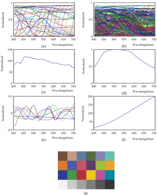
62
optimizing the spectral sensitivity of broadband multispectral camera by FVAM simply.
63
The article is arranged as follows. We introduce MLI filter selection methods in section 2. Then
64
experimental simulation was conducted in section 3. We abstract the features of the best-performed
65
filter set from the results of the experimental simulation in section 4. We discuss the generalization of
66
the results of the article in section 5.The conclusion is drawn in section 6.
67
2. MLI filter selection method
68
Contrasting to the SRM, the FVAM can be conducted by merely analyzing the features of filter
69
transmittance vectors without considering specific linear model 1 of multispectral camera, which
70
contains all the factors affecting the response of the camera sensor. The FVAM works well only if
71
some mathematical measurements for spectral transmittances of corresponding filter set is
72
competent for color reproduction or spectral reconstruction precisely, regardless of other camera
73
parameters.1, 7, 8
74
In Ref. 1 and Ref. 8 ,several types of filters are considered to optimize the spectral sensitivity of
75
multispectral camera by comparing their performances, including narrowband filters pairs of
76
isolated Gaussian curve shape VS overlapped Gaussian curve shape, and both of broadband and
77
narrowband filters selected by different selection methods of the MLI VS the Maximum Orthogonality
78
Method (MOM). The results show that the overlapped filter set and filter set selected by MLI perform
79
better. With same number of channels, broadband commercial available absorption filter sets
80
selected by MLI performs better than the interference narrow ones. From the previous researches,
81
we have shown that the broadband multispectral camera is more effective than narrowband ones
82
with same number of spectral channels , and that transferring application of MLI from training set
83
selection to filter selection has a great potential to further exploration.1, 8, 10
84
The original proposal of MLI used in multispectral color imaging is relevant to training set
85
selection, seeking minimum numbers spectral samples in a large set of collection for the most
86
representative subset.9 From the perspective of linear algebra, that means the sample subset selected
87
spans as uniformly as possible in the overall spectral space. Multispectral camera model is this:
88
[diag(L)⋅diag(S)⋅T]TR=C (1)
89
where the diag(. ) denotes a diagonal matrix with elements of corresponding vector, and [.]T denotes
90
transpose of a matrix;
91
L=[l1 li ln]T (2)
92
is a column vector of light source spectral distribution with each elements corresponding to a
93
wavelength sample;
94
S=[s1 si sn]T (3)
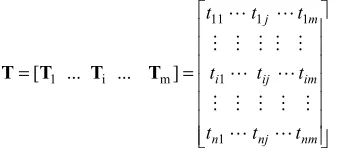
95
= = nm nj n im ij i m j t t t t t t t t t 1 1 1 1 11 m i
1 ... ... ]
[T T T
T (4)
97
is a matrix of spectral distribution of filter transmittances with m spectral sensing channels, each
98
column of which is a transmittance vector of a corresponding filter corresponding with n
99
wavelength sample; R andCis column vector of reflectance and response of camera sensor
100
respectively. Let
101
Φ=[diag(L)⋅diag(S)⋅T]T, (5)
102
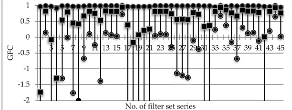
we can see the camera model describes a linear transform from Eq.1 to Eq.5.
103
From the above model, Φ should be an orthogonal matrix if the R can be precisely
104
reconstructed. However, we wonder if MLI method could be an effective method for filter selection
105
due to its independence to other camera parameters .If for sure, it can be helpful for setting up an
106
optimized multispectral imaging camera.
107
The algorithm to select broadband filters by MLI is listed in Figure 1. The aim of the algorithm
108
is to select filter sets which transmittances matrix has the minimum condition number. From Figure
109
1, we can see that the first selected filter is supposed to be the one which corresponding vector has
110
the maximum ℓ norm; it would lead to the highest signal to noise rate in the first channel as
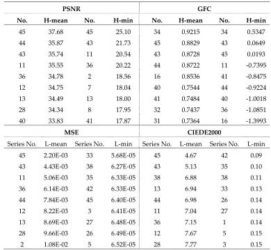
111
expected. However, there exists that the next selected filters may contain the filter with highest value
112
of ℓ norm possibly if the first filter is not the maximum ℓ norm, that is to say, a highest signal to
113
noise needed not to be gained by the first channel of the broadband multispectral camera logically.
114
That will be verified by the following experimental simulation in section 3, where we will show that
115
the best-performed filter set is often not the first filter with maximum ℓ norm.
116
117
118
Figure 1. Algorithm for select broadband filters by Maximum Linearity Independence method (MLI).
119
3. Experimental simulation
120
3.1. Datasets
121
In the next imaging simulation, datasets comprise transmittances of filter sets, spectral
122
sensitivity of camera, illuminant and spectral cubic images. The filter datasets are obtained from
123
datasheet of color filter glass of Hoya Group [12], which has 45 single filter transmittances (see
124
Figure 2a). The physical constraints of the thickness and the transmittance of a filter must be
125
concerned, because it would not be practical due to the thickness and transmitted energy if the
126
number of the filters that stack up to form a filter combination is larger than 2. Therefore, let K
127
denotes the number of transmittances that can be selected from the collection, which comprise single
128
filters and combinations of two filters; and N denotes the number of original transmittance, then
129
=1035 )! 2 45 ( ! 2 ! 45 452 = + −
+ =N N
K . (6)
130
The 1035 transmittances are illustrated in Figure 2b. The CIE standard illuminant D65 and
131
camera sensitivity of Basler 302f are displayed in Figure 2c/d. The spectral data cube with
132
Task: Find filter set of M channels with minimum condition number among K (a large number) transmittances
Step 0: Collect transmittance vector sets ( ) which comprise K transmittances;
Step 1: S=1, select transmittance vector which ℓ norm is maximum value from ;
Step 2: S=2, select transmittance vector from rest vectors in which satisfies transmittance matrix, [ T , T], has minimum condition number;
… …
320*582=186240 voxels (the axis of “Voxels” are the position coordinates for x,y and the spectral
133
coordinate for reflectance) ,which is formed by 24 reflectance spectrums derived from spectral
134
measurements of 24 patches of Macbeth Color Checker; each patch of which comprises 80*97
135
voxels(see Figure 2g for its 2D display). All the spectral data contain 61 spectral measurements
136
evenly sampled in wavelength range from 400-700 nm.
137
138
139
Figure 2. Visualization of data sets used for simulation. (a) Transmittances of 45 single filters. (b) All
140
1035 transmittances of single filters and two single filter combinations (c) Spectral distribution of
141
CIE standard illuminant D65. (d) Camera sensitivity of Basler 302f camera sensor.(e) The first
142
eigenvectors of spectral data of Macbeth ColorChecker.(f) Spectral distribution of CIE standard
143
illuminant A. (g) Color display of spectral data cubic of Macbeth Color Checker.
144
3.2. Experimental simulation
145
Taking each of the 45 single filters for the first filter of every desired series of selected filter set,
146
other filters of the intended filter set are selected from the rest of 1034 filter transmittances according
147
to algorithm listed in Figure 1; The corresponding condition numbers of the selected filter sets
148
are computed at the same time. In the following, the word ‘No. of filter’ is defined as the serial
149
number of the single 45 filters, and the ‘No. of filter set series’ means a filter set series containing 4
150
to 8 filter channels of which the first filter is form the sequential 45 filters.
151
400 450 500 550 600 650 700
0 0.5 1
Wavelength/nm
(a)
No
rm
a
li
z
ed
400 450 500 550 600 650 700
0 0.5 1
Wavelength/nm
(b)
No
rm
a
li
z
ed
400 450 500 550 600 650 700
0 50 100 150
Wavelength/nm
(c)
No
rm
a
liz
ed
400 450 500 550 600 650 700
0 0.5 1
Wavelength/nm
(d)
No
rm
a
liz
ed
400 450 500 550 600 650 700
-0.5 0 0.5
Wavelength/nm
(e)
No
rm
a
liz
ed
400 450 500 550 600 650 700
0 50 100 150 200
Wavelength/nm
(f)
No
rm
a
liz
ed
For every selected filter sets, imaging simulation below comprises three steps. Firstly, we
152
compute the camera response image (CResponse) of the original reflectance image (ROriginal) by
153
adding Gaussian noise (NGaussian) according to Eq.7:
154
CResponse=([diag(L)diag(S)T]TROriginal)T+NGaussian. (7)
155
Secondly, reconstructed spectral image (RRecounstruct) is computed according to Eq.8:
156
RRecounstruct=ψ0pinv(([diag(L)diag(S)T]TROriginal)Tψ0)CResponse , (8)
157
Where pinv(.) denotes pseudoinverse of a matrix, and ψ0is a matrix which columns are the first m
158
eigenvectors of the spectral reflectance of Macbeth ColorChecker (m is the number of channels of
159
multispectral camera).More generally speaking, ψ0 represents the priori information of the
160
reflectance of the imaging scene. Maloney and Wandell used the reconstruction algorithm for the
161
first time, into which the insight is making use of linear approximation for the reflectance by the
162
basis vectors of the priori spectral training set [13, 14]. Finally, we evaluate the performance of
163
spectral reconstruction relevant to the selected filter sets.
164
As we know, a single index is not capable of evaluating both the performance of spectral
165
reconstruction and color reproduction in multispectral imaging. Therefore, several indices, such as
166
PSNR, GFC, CIECDE2000 and MSE often employed in multispectral community, 2, 15-17 are adopted to
167
appraise the performances of the selected filter sets. Considering the relatively excellent results in
168
the following simulation computed by the expression of GFC used in literatures [16 ,17] are almost
169
equal to 1, that is to say, losing its discrimination, the embedded Matlab function of GoodnessofFit are
170
adopted to compute GFC .The formula is as follows:
171
GFC = 1 − −
− , 9
172
where the cost function is normalized root mean square error (NMSE) of the estimated ( ) and the
173
reference vector ( ). The NMSE costs vary between –Inf. (bad fit) to 1(perfect fit).Generally, the
174
higher of PSNR, the more of GFC close to 1, the more of CIEDE2000 and MSE are approach to 0 ,
175
the performance of corresponding filter sets is more optimal. Note that the GFCs in this article are
176
calculated by Matlab function goodnessOfFit (RMSE) [18].
177
In the simulation, we adopt five channel numbers of multispectral camera; the numbers of
178
spectral channels are 4, 5, 6, 7 and 8 respectively. The level of additive Gaussian noise denoted by
179
SNR (signal to noise rate) is varied by the ten noise levels in DBs, where SNR∈[∞, 50, 47, 43, 40, 37,
180
33, 30, 27, 23].The relationship of SNR and the noise variance is defined by
181
σ = 10 , (10)
182
The noise is added by the imnoise Matlab function to the response image CResponse described in
183
Eq.7.
184
4. Results and analysis
185
4.1 Data reduction
186
From the simulation, we acquired 2250 groups of results for investigation. Each of them is
187
relevant to a number of channels and a noise levels, and contains four evaluation indices that are
188
PNSR, GFC, CIEDE2000 and MSE. From the results, the performances of the filter sets are generally
189
consistent with each other in that the higher SNR of noise level and the channel number are the
190
better performance of the filter set series is. We can take the GFCs of the first four filter sets for
191
example (see Figure 3). From Figure 3, we can see the performances of the filter sets with different
192
series numbers differ from each other distinctly, and the general trends of performance when
193
varying the number of channels and noise levels. However, we can hardly recognize the specific
194
best-performed filter set among so much of items. It is necessary to find a measurement to evaluate
195
197
Figure 3. The GFCs of the first four filter series (only positive values are displayed for clarity),where
198
each of the four groups of stems presents the performance of the corresponding filter sets under ten
199
noise levels and four number of channels. From the left to the right of each group, ten clusters of
200
stems illustrate the GFCs in terms of different noise levels in descending order; each of the clusters
201
contains five numbers of the channels of multispectral camera. The numbers of channels are 8,7,6,5
202
and 4 from the left to the right.
203
We have computed the mean, maximum and minimum of all the 50 datasets relevant to each
204
one filter set series. Fig.4 shows the overall performances of the 45 series of filter sets in terms of
205
GFC, where the upper round marker denotes the maximum value; the middle square denotes the
206
mean; and the lower round denotes the minimum (some of the minimums with negative value less
207
than -2 are not displayed). We can see which series of filter sets performance better intuitively. So
208
does the filter sets with specific channels, as we can see that in Fig. 5. Those in terms of other
209
evaluation indices have similar characteristics, which are omitted here for clarity.
210
211
Figure 4. Overall performances of the 45 series of filter sets in terms of GFC.
212
213
Figure 5. Overall performances of the 45 series of filter sets for 6 channels in terms of GFC.
214
As we have known, we cannot tell which filter set performs better by only one index. However,
215
if a filter set has the maximum frequency out of the best-performance filter sets collection in terms of
216
different indices, we can reasonably conclude that the filter set is the best one. Therefore, we collect
217
the top best-performed filter sets (for 20% in this article) in terms of the entire four indices to find the
218
largest frequency of a filter set getting involved.
219
0 0.2 0.4 0.6 0.8 1
1 3 5 7 9 11 13 15 17 19 21 23 25 27 29 31 33 35 37 39
GFC
No. of filter set series
-2 -1.5 -1 -0.5 0 0.5 1
1 3 5 7 9 11 13 15 17 19 21 23 25 27 29 31 33 35 37 39 41 43 45
GFC
No. of filter set series
-2 -1.5 -1 -0.5 0 0.5 1
1 3 5 7 9 11 13 15 17 19 21 23 25 27 29 31 33 35 37 39 41 43 45
GFC
4.2 Data sorting and the best-performed selection with overall channels
220
Table.1 Statistics of the top 20% best-performed filter set series.
221
PSNR GFC
No. H-mean No. H-min No. H-mean No. H-min
45 37.68 45 25.10 34 0.9215 34 0.5347 44 35.87 43 21.73 45 0.8829 43 0.0649 43 35.74 11 20.54 43 0.8728 45 0.0193 11 35.55 36 20.22 44 0.8722 11 -0.7395 36 34.78 2 18.56 16 0.8536 41 -0.8475 12 34.75 7 18.04 40 0.7544 44 -0.9224 13 34.49 13 18.00 41 0.7484 40 -1.0018 28 34.34 8 17.95 32 0.7437 36 -1.0851 40 33.83 41 17.87 31 0.7364 16 -1.3993
MSE CIEDE2000
Series No. L-mean Series No. L-min Series No. L-mean Series No. L-min 45 2.20E-03 33 5.68E-05 45 4.67 42 0.09 43 4.43E-03 38 6.27E-05 43 5.13 35 0.10 11 5.06E-03 35 6.33E-05 38 6.88 38 0.11 36 6.14E-03 42 6.33E-05 13 6.94 33 0.13 44 7.84E-03 45 6.40E-05 44 6.98 26 0.14 12 8.22E-03 3 6.41E-05 11 7.04 27 0.14 13 8.69E-03 27 6.48E-05 36 7.15 1 0.14 28 9.66E-03 26 6.49E-05 12 7.67 5 0.15 2 1.08E-02 5 6.52E-05 28 7.77 3 0.15
Table 1 list the results of the top 20% best-performed filter sets in terms of PSNR, GFC,
222
MSE,CIEDE2000, where the data of PSNR and GFC are sorted in descend way, and those of MSE
223
and CIEDE2000 are sorted in ascend way. All the data are derived from their corresponding
224
averages of each index, which include those of all the 10 noise levels and all the channel numbers of
225
the filter set series. In table 1, the No. denotes the No. of filter set series; H-mean denotes descend
226
order of the means; H-min denotes descend order of the minimums; L-mean denotes ascend order
227
of the means and L-min denotes ascend order of the minimums. From table 1, we can see the order
228
of the sorted data relevant to each specific filter set series is not consistent; however, there are some
229
appearing frequently. For convenient, we count the frequency of the each emerged filter set series,
230
the results are demonstrated in Figure 6 (a).From Figure 6 (a),we can see the No.45 have the most
231
frequency in the nine best-performed results, and the No.11,43,44 rank the second place. Moreover,
232
we can see from table 1 and Fig. 6 (a) that the No.2 filter set series in which the transmittance vector
233
of the first filter has the maximum norm is not the best-performed filter set series.
234
Another method to decide explicitly which filter set being more optimal is score ranking
235
method. The score ranking method is designed like this: Let the first filter series in table 1 having the
236
highest score of 9, the second having 8 and so on, then we can get the cumulated scores of the filter
237
sets series. The results are figured in Fig. 6 (b).From Fig. 6(b), we can see that the above the No.11,43
238
Especially, if there is not just one filter set series sharing a same maximum frequency, the score
240
ranking method may be irreplaceable.
241
242
(a) (b)
243
Figure.6 Statistics of the best-performed filter set series. (a) Frequency ; (b) Accumulative scores.
244
4.3 Best-performed selection with single channel number
245
We have computed statistics of the top 20% best-performed filter sets with 4-8 channels respectively
246
in terms of PSNR, GFC, MSE, and CIEDE2000.All the data are derived from their corresponding
247
averages of each index, which comprise those with all the 10 noise levels. In this section, we give
248
the performances of filter sets in terms of different channel numbers. The data are processed by
249
score ranking method in the same way as in section 4.2, and the results together with those of the
250
overall channels in section 4.2 are listed in table 2, where the best-performed filter set series and the
251
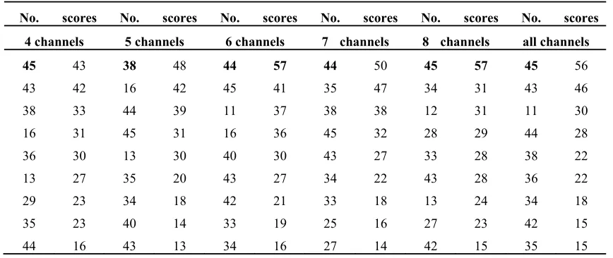
highest cumulative scores are printed in bold.
252
Table 2. Accumulative scores of the nine best-performed filter sets or series with D65.
253
No. scores No. scores No. scores No. scores No. scores No. scores 4 channels 5 channels 6 channels 7 channels 8 channels all channels
45 43 38 48 44 57 44 50 45 57 45 56
43 42 16 42 45 41 35 47 34 31 43 46
38 33 44 39 11 37 38 38 12 31 11 30
16 31 45 31 16 36 45 32 28 29 44 28
36 30 13 30 40 30 43 27 33 28 38 22
13 27 35 20 43 27 34 22 43 28 36 22
29 23 34 18 42 21 33 18 13 24 34 18
35 23 40 14 33 19 25 16 27 23 42 15
44 16 43 13 34 16 27 14 42 15 35 15
4.4 Comparison with the performance of best selection and the past selection
254
We have computed the norms for the transmittance vectors of the 45 filters, and revealed
255
that that of the No.2 filter was the maximum. From table 2, we can see the No.44 and 45 filter set
256
series have same maximum accumulative scores (57). But the No. 44 filter set series has the
257
maximum accumulative scores and a smaller number of channels (6 channels) comparing with those
258
1 5 10 15 20 25 30 35 40 45
0 1 2 3 4 5 6 7
No. of filter set series
Fr
eq
u
en
cy
1 5 10 15 20 25 30 35 40 45
0 10 20 30 40 50 60
No. of filter series
A
ccu
m
u
la
te
s
co
of the No.45 filter set series (8 channels). Therefore, we display the results of the No.44 and No.2
259
filter set series with 6 channels in table 3 for comparison. From table 3, we can see the performance of
260
the No.44 is greatly improved comparing to the No.2 .The same conclusion can also be made from
261
table 2, in which all the filter set series listed outperform the No.2 filter set series.
262
Table 3. Performance of the best-performed filter set and the past selection one for 6 channels.
263
Indices PSNR GFC MSE DE2000
No. 44 2 44 2 44 2 44 2 Average 38.434 32.11 0.9318 0.1617 2.39E-03 1.72E-02 4.13 10.494
4.5 Presentation of the best performed MLI filter sets with different noise
264
From table 2, we can see the best filter set selected by MLI, however the specific performance of
265
those filter sets at each noise level may be meaningful to practical application. Table 4 lists the results
266
of performance for the filter sets. From table 4, we can see the performance of each best filter set at
267
specific noise level, which can be a quantitative reference for practical applications.
268
Table.4 Performances of the best filter sets.
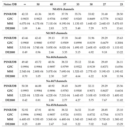
269
Noise /DB ∞ 50 40 37 33 30 27 23
N0.45/4 channels
PSNR/DB 42.33 41.36 38.95 37.78 35.76 33.82 31.68 28.50
GFC 0.9835 0.9823 0.9704 0.9587 0.9245 0.8689 0.7778 0.5422 MSE 6.07E-04 6.17E-04 7.11E-04 8.19E-04 1.13E-03 1.64E-03 2.64E-03 5.47E-03
DE2000 1.09 1.46 2.83 3.72 5.48 7.29 9.73 13.61
N0.38/5 channels
PSNR/DB 43.46 42.41 39.13 37.35 34.40 31.96 29.29 25.63
GFC 0.9900 0.9880 0.9707 0.9509 0.8998 0.8159 0.6679 0.3004 MSE 3.51E-04 3.74E-04 5.85E-04 8.02E-04 1.49E-03 2.60E-03 4.82E-03 1.11E-02
DE2000 0.49 0.96 2.46 3.35 5.15 6.92 9.18 13.22
No.44/6channels
PSNR/DB 49.40 45.72 40.56 38.33 35.12 32.46 29.69 26.11
GFC 0.9994 0.9984 0.9897 0.9799 0.9522 0.9139 0.8371 0.6556 MSE 2.54E-04 2.80E-04 5.07E-04 7.69E-04 1.52E-03 2.77E-03 5.19E-03 1.19E-02
DE2000 0.70 1.05 2.30 3.07 4.64 6.22 8.38 11.94
No.44/7channels
PSNR/DB 50.38 46.88 40.92 38.45 34.89 32.11 29.29 25.56
GFC 0.9993 0.9984 0.9896 0.9783 0.9500 0.9071 0.8437 0.6634 MSE 1.22E-04 1.52E-04 4.22E-04 7.21E-04 1.64E-03 3.10E-03 5.93E-03 1.40E-02
DE2000 0.42 0.81 2.06 2.77 4.27 5.75 7.67 11.02
No.45/8channels
PSNR/DB 52.92 47.91 40.94 38.32 34.52 31.69 28.85 25.10
GFC 0.9996 0.9982 0.9857 0.9724 0.9331 0.8732 0.7764 0.5173 MSE 6.40E-05 9.35E-05 3.56E-04 6.48E-04 1.54E-03 2.96E-03 5.73E-03 1.38E-02
4.6 Characteristics of the best-performed MLI filter sets
270
The condition numbers of the best-performed filter set series and those of No.2 series are listed
271
in table 5, where the figures printed in bold are condition number of the filter sets with the
272
best-performed channels. The condition numbers of the entire filter set series are displayed in Fig.7
273
by radar charts.
274
From table 5, the condition numbers of the best filter sets is less than 4, although the condition
275
numbers are not always the minimum for the best-performed filter set. From Fig7, we can see the
276
condition numbers listed in table 5 are one of the several smallest among all the condition numbers.
277
Therefore, it indicates that minimizing the condition number of a filter set is an essential
278
precondition for optimizing the sensitivity of broadband camera, and the best-performed filter set
279
must be the one with a smaller condition number than most of the condition numbers of the others.
280
Table 5. Condition numbers of the best-performed filter set and the conventional selection.
281
Channels No.45 No.38 No.44 No.2
4 1.45 1.65 1.37 5.84
5 2.11 2.56 1.63 6.65 6 2.55 3.21 2.31 9.74 7 3.04 3.91 3.10 12.01
282
283
284
Figure 7. The condition numbers versus the corresponding filter sets and channel numbers.
285
The radical coordinates denote condition numbers and the angular coordinates denote the
286
No. of the filter sets, therefore the square markers denote the position of the corresponding
287
filter sets. In the radar charts for 7 and 8 channels, some of the condition numbers cannot
288
be seen because they are too large to be displayed and we are more concern with the
289
smaller ones.290
0 1 2 3 4 5 6 1 2 3 45 6 7 8 9 10 11 12 13 14 15 16 17 18 19 20 21 22 23 24 25 26 27 28 29 30 31 32 33 34 35 36 37 38 39 4041 4243 44
45 4 Channels 0 2 4 6 8
10 1 2 3 4 5 6 7 8 9 10 11 12 13 14 15 16 17 18 19 20 21 22 23 24 25 26 27 28 29 30 31 32 33 34 35 36 37 3839 4041 424344 45 6 Channels 0 1 2 3 4 5 6 7
8 1 2 3 4 5 6 7 8 9 10 11 12 13 14 15 16 17 18 19 20 21 22 23 24 25 26 27 28 29 30 31 32 33 34 3536 3738 3940 414243 44 45 5 Channels 0 2 4 6 8 10 12 1 2 3 4
5 6 7 8 9 10 11 12 13 14 15 16 17 18 19 20 21 22 23 24 25 26 27 28 29 30 31 32 33 34 35 36 37 38 3940 4142 43 4445
7 Channels 0 4 8 12 16 20 24 1 2 3 4
5 6 7 8 9 10 11 12 13 14 15 16 17 18 19 20 21 22 23 24 25 26 27 28 29 30 31 32 33 34 35 36 37 3839 4041
4243 44 45
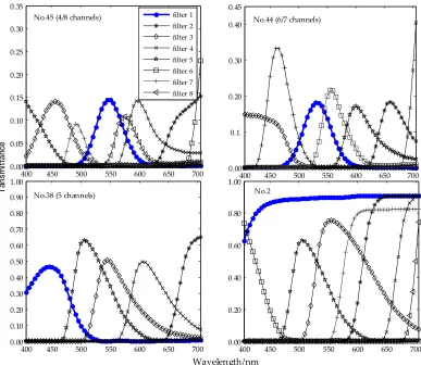
For further investigation, the transmittances of the best-performed filter sets in table 4 are
291
graphed in Fig. 8, where the first filter of the filter sets is graphed in bold line with round markers.
292
Comparing to No. 2, we can see that the first filter of the best set has a distinct transmittance peak
293
and the peaks of the sequential filters distribute almost evenly in the wavelength range. Comparing
294
No.38 and No.45 or N.44 when the No. of channels equals 5, we can see that the best filter set (No.38)
295
has higher transmittances and more overlaps than the first five channels of No.44 or No.45. Similarly,
296
we can see the consistent geometric distribution of the first 4 filters of best performed No.45 filter set
297
versus that of the No.44.Especially we can see there is a large notch in wavelength from 580nm to
298
630nm or so, which may be the cause of No.44 has worse performance than No.45 at the channels
299
number being equal to 4.
300
301
Figure 8. Transmittances of the best-performed filter sets (from No.45, 44 and 38) and the filter set
302
series with maximum ℓ norm first filter (No.2).
303
5. Discussion
304
5.1 General applicability of the MLI method with varying imaging parameters
305
We have revealed the characteristics of the best-performed filter sets from above simulation;
306
however, we want to know its general applicability when changing the camera parameters,
307
especially varying the illuminant. Among the parameters related in section 2, the imaging
308
illuminant is varying easily under real condition, for example, lighting uncontrollable outdoor
309
imaging. Therefore, we make another simulation with the CIE standard A illuminant graphed in
310
Fig.2f. The results correspond to table 2 are listed in table 6,which display the accumulative scores
311
0 0.2 0.4 0.6 0.8 1 0
0.2 0.4 0.6 0.8 1
400 450 500 550 600 650 700
0.00 0.05 0.10 0.15 0.20 0.25 0.30 0.35
T
ansm
it
tan
ce
400 450 500 550 600 650 700
0.00 0.1. 0.20 0.30 0.40 0.45
400 450 500 550 600 650 700
0.00 0.10 0.20 0.30 0.40 0.50 0.60 0.70 0.80 0.90 1.00
No.38 (5 channels)
400 450 500 550 600 650 700
0.00 0.20 0.40 0.60 0.80 1.00
Wavelength/nm No.2 filter 1
filter 2 filter 3 filter 4 filter 5 filter 6 filter 7 filter 8
of the first four best-performed filter sets or series with A illuminant; and the performance of the
312
best-performed filters in A illuminant are listed in table 7.
313
Table 6. Accumulative scores of the four best-performed filter sets or series with A illuminant.
314
No. scores No. scores No. scores No. scores No. scores
4 channels 5 channels 6 channels 7 channels 8 channels
45 43 16 50 44 52 44 50 45 57
43 40 38 42 45 43 35 46 34 31
16 36 45 39 16 38 38 37 12 31
38 33 44 37 34 31 45 31 28 29
Table.7 Performances with A illuminant of the best filter sets.
Noise /DB ∞ 50 40 37 33 30 27 23
N0.45/4 channels
PSNR/DB 41.97 40.97 38.48 37.16 35.07 33.09 30.96 27.67
GFC 0.9867 0.9855 0.9737 0.9612 0.9216 0.8731 0.7819 0.5020 MSE 6.63E-04 6.76E-04 7.94E-04 9.30E-04 1.32E-03 1.97E-03 3.21E-03 6.81E-03
DE2000 0.65 1.02 2.42 3.28 4.52 5.68 7.00 8.85
N0.16/5 channels
PSNR/DB 43.46 42.41 39.13 37.35 34.4 31.96 29.29 25.63
GFC 0.9989 0.9981 0.9905 0.9824 0.9584 0.9259 0.8625 0.6799 MSE 6.32E-04 6.52E-04 8.25E-04 1.01E-03 1.57E-03 2.49E-03 4.30E-03 9.44E-03
DE2000 0.93 3.45 8.42 10.18 13.15 14.49 15.59 16.00
No.44/6channels
PSNR/DB 40.86929 40.40447 38.37405 37.17598 34.85175 32.74033 30.30314 26.85012 GFC 0.9994 0.9984 0.9896 0.9799 0.9487 0.9140 0.8413 0.6685 MSE 3.12E-04 3.52E-04 7.07E-04 1.08E-03 2.25E-03 4.06E-03 7.81E-03 1.84E-02
DE2000 0.66 0.93 2.15 2.94 4.04 5.20 6.47 8.31
No.44/7channels
PSNR/DB 49.84912 45.72807 39.52636 37.02057 33.49637 30.69482 27.7842 24.08812 GFC 0.9994 0.9985 0.9896 0.9804 0.9529 0.9099 0.8386 0.6561 MSE 1.38E-04 1.86E-04 6.01E-04 1.08E-03 2.47E-03 4.77E-03 9.33E-03 2.21E-02
DE2000 0.43 0.80 2.04 2.73 3.82 4.79 6.04 7.59
No.45/8channels
PSNR/DB 53.17 47.32 39.78 37.13 33.32 30.42 27.56 23.71
GFC 0.9996 0.9982 0.9845 0.9700 0.9245 0.8718 0.7596 0.4668 MSE 6.68E-05 1.08E-04 4.79E-04 8.76E-04 2.10E-03 4.08E-03 7.96E-03 1.93E-02
DE2000 0.41 1.00 2.54 3.28 4.65 5.90 7.33 9.44
Comparing to table 4, the best-performed filter set in table 6 are almost the same at the
315
number of channels equaling to 4, 6, 7 and 8, although the different light source was used. An
316
exception is the No.16 filter set at the number channels equals 5. The transmittance curves of No.16
317
8.Comparing the curves from Fig. 9 with those of Fig. 8, the same conclusions can be made with
319
No.16 as that of N0.38, and so do the condition numbers in table 7. Form the ranking cumulate score
320
table (see table 8), in fact, we can see No.38 is the closest 5 channels filter set just behind the
321
best-performed, No.16 filter set. The performance is slightly better in A illuminant than that of D65
322
comparing table 2 to table 8, however the best performed filter are still those with smaller condition
323
numbers and characteristics of curve shapes . The facts that the best-performed filter sets with CIE A
324
illuminate support our conclusion about the criterions to the best-performed filter sets derived from
325
those with CIE D65 illuminate. In other word, the criterions to select filter set to optimizing the
326
spectral sensitivity of broadband camera is independent to the imaging parameter, light source,
327
which illuminate the imaging scene.
328
329
Figure 9. Transmittances of the best-performed filter set, No.16 (5).
330
Other imaging parameters may be changed for similar simulation such as varying the camera
331
spectral sensitivity function and the spectral imaging scene; unfortunately, there remains no more
332
necessary energy to do that. The generalization of the conclusions about the criterion of the
333
competent filter set selected by MLI would be justified by the simulations with varying the light
334
source above.
335
5.2 Two intuitive steps for MLI method to selecting filter sets
336
From the simulation above, we can select the best filter set for optimizing the sensitivity of
337
broadband multispectral camera by the characteristics such as the condition number and the
338
geometric distribution of the transmittance curves. However, the methodology is intuitive and still
339
difficult to operate in practice. The reasons lie in two aspects.
340
The one is that the best-performed filter set is not always the one with the smallest condition
341
number as it can been seen in table 5 and from comparison between table 2, table 7 and Fig.7.The
342
other is that the characteristics of the transmittance curves of the filter set is too intuitive to be
343
handled quantitatively. Therefore, we recommend two steps to obstacle the problem.
344
The first step is to select a subset of the filter sets with smaller condition number from the
345
entire filter sets. Comparing table 2 and table 7 to Fig.7, we can see the best-performed filter set
346
stays among several filter sets with the smallest condition numbers. Table 8 list the ordinal numbers
347
of condition number sorted from small to large among 45 corresponding condition numbers for
348
the best-performed filter sets. From table 8 we can see that the condition numbers of the
349
best-performed filter sets are almost the closest to the most smallest; the farthest is condition
350
numbers of No. 38 filter set, of which the ordinal number is 5 in all the 45 filter sets. Namely, if the
351
400 450 500 550 600 650 700 0.00
0.10 0.20 0.30 0.40 0.50 0.60 0.70 0.80
Wavelength/nm
Ta
n
sm
it
ta
n
ce
subset of filter sets is composed by the 5 filter sets with the smallest condition number, we can
352
decide the best-performed filter set is in it.
353
The second step is to select a filter set among the subset in terms of the geometric distribution
354
of its transmittance curves or by a few experimental explorations. The geometric distribution of the
355
transmittance curves of a best-performed filter sets related above would give an intuitive criterion
356
to identify the best-performed filter set from the subset conveniently, otherwise experimental
357
explorations can be conducted with every filter set in the subset to pick out the best-performed filter
358
set according the experimental results. Because of the number of the filter sets in the subset is less
359
than five according to the results of this article, it would also be an efficient way to select the
360
best-performed filter set in the subset .
361
Table 8. Ordinal number of the condition numbers of the best-performed filter sets with different
362
illuminant.
363
Channels 4 5 6 7 8
Filter No. 45 38 44 44 45 D65 3 5 2 2 1 Filter No. 45 16 44 44 45
A 3 1 2 2 1
364
So far, we have investigated selecting broadband filter set from a large number of commercial
365
filters to optimizing the spectral sensitivity of broadband multispectral imaging camera by imaging
366
simulation. From the results of the simulation, we found the remarkable characteristics of the
367
best-performed filter set. Besides smaller condition number of the best-performed filter set, the
368
geometric features of it comprise the distinct peak of the transmittance of the first filter, the
369
generally uniform distributing of the peaks of the transmittance curve of the filters and the
370
substantial overlapping of the transmittance curves with those of the adjacent filer sets.
371
It is worth noting that one reason of only selecting 45 single filters from1035 filters as the first
372
filter is to reduce the calculating pressure, and the other is that the single filter is easier to
373
implement than the combinations in practice application. Other 990 filters achieved by combination
374
of two single filters may be serving as the first filter; it would produce more filter set series for
375
selected by the MLI method related above, therefore it would lead the spectral sensitivity of
376
broadband multispectral camera to be more optimizing.
377
Although derived by the simulation with glass transmittance filters illustrated in Fig. 1a, the
378
results of this paper can applied to other types of filters, for example, the transmittance design of
379
SFA (spectral filter array) multispectral system. We can see it as an experimental explanation to
380
answer why the spectral transmittances would make it work well for SFA multispectral system.7, 19
381
6. Conclusions
382
Vector analysis method for selecting broadband filters is an efficient way to optimal spectral
383
sensitivity of multispectral camera without time-consuming imaging simulation or experiments
384
from commercial filters. In this paper, we introduced the background strategy and the algorithm of
385
the MLI filter selection method; we questioned the reason why the first filter is selected by the
386
maximum ℓ norm of its transmittance vector. Then we conducted an exhaustive simulation
387
searching for the best-performed filter set based on MLI by varying the first filter selected in turn
388
from the entire single-chip broadband filter collection. From the results of the simulation, we found
389
that there are filter sets selected by MLI outperforming the filter set selected by MLI with maximum
390
ℓ norm filter serving as the first selected filter as expected. The optimal filter set has distinct
391
characteristics of smaller condition number and remarkable geometry characteristics, such as
392
distinct peak of the transmittance of the first filter, generally uniform distributing of the peaks of the
393
of the adjacent filer sets. The characteristics can serve as an intuitive criterion of filter vector
395
analyzing method for optimizing the broadband multispectral imaging sensors or the spectral
396
sensitivity of SFA sensors due to considering the variation of the noise conditions in the
397
experimental simulation. As a future work, the characteristics of the best-performed filter set
398
selected by MLI vector analyzing method may be modeled mathematically such that a more
399
precisely described criterion for broadband filter selection by MLI would be put forward;
400
furthermore, the criterion would be investigated with actual experiments using real camera(s),
401
tested in an actual scenario.
402
403
Acknowledgments: The work was supported by the Talent Introduction research foundation of Binzhou
404
University (No.801001021616), the Dual Targets for regional and industrial research foundation of Binzhou
405
University (No.BZXYHZ20161008) and the Key Project Foundation of High Definition Satellite of CCRSDA.
406
Author Contributions: Sui-Xian Liwrote the manuscript and was responsible for the research design, data
407
collection, and analysis. A-Qi Xu,Li-Yan Zhang and Jun Lin assisted in methodology development and
408
research design and participated in the writing of manuscript and its revision.
409
Conflicts of Interest: The authors declare no conflict of interest.
410
References
411
1. Li Suixian; Zhang Liyan. Optimal Sensitivity Design of Multispectral Camera Via Broadband Absorption
412
Filters Based on Compressed Sensing. Springer Proceedings in Physics, vol. 192, 3rd International
413
Symposium of Space Optical Instruments and Applications, Beijing, China, Sep. 26-29,2016;Urbach H.,
414
Zhang G. ,Eds. Springer, Cham,Switzerland,2017 .(DOI:10.1007/978-3-319-49184-4_33)
415
2. Shrestha, R; J. Y. Hardeberg. Spectrogenic imaging: a novel approach to multispectral imaging in an
416
uncontrolled environment. Opt. Express 2014, 22(8),pp.9123-33.
417
3. J. Y. Hardeberg. Filter Selection for Multispectral Color Image Acquisition. ImagingSci.Techn.2004,
418
48(2),pp.177-182.
419
4. F. H. Imai; S. Quan; M. R. Rosen; R. S. Berns. Digital camera filter design for colorimetric and spectral
420
accuracy. Proc. of 3rd International Conference on Multispectral Color Science,,pp13-16,University of
421
Joensuu,Finland,2001.
422
5. D. Y. Ng; J. P. Allebach. A subspace matching color filter design methodology for a multispectral imaging
423
system. IEEE T Image Process,2006,15(9), pp.2631– 2643.
424
6. S. Quan; N. Ohta; N. Katoh. Optimization of camera spectral sensitivities. Proc. of the IS&T and SID 8th
425
Color Imaging Conference, pp. 273-277, IS&T, Springfield, VA, 2000.
426
7. P. L. Vora; H. J. Trussell. Measure of goodness of a set of color-scanning filters. J. Opt. Soc. Am. A,1993,
427
10(7), pp.1499-1503.
428
8. S. X. Li; N. F. Liao; Y. N. Sun. Optimal Sensitivity of Multispectral imaging system based on PCA,
429
Opto-Electronic Engineering (published in Chinese),2006,33(3),pp.127-132.
430
9. J. Y.Hardeberg. Acquisition and Reproduction of Color Image: Colorimetric and Multispectral
431
Approaches, ISBN: 1-58112-135-0, Http://www.dissertation.com,USA,2001.
432
10. Li Suixian. Several problems research of multispectral imaging, Dissertation for PHD degree (published in
433
Chinese),Beijing institute of technology,2007.
434
11. R.Shrestha;J.Y.Hardeberg. Multispectral imaging using LED illumination and an RGB camera.21st Color
435
and Imaging Conference Final Program and Proceedings, Society for Imaging Science and
436
Technology,pp.8-13,2013.
437
12. URL:http://www.hoyaoptics.com/color_filter.Hoyo corporation USA optical division.
438
13. L. T. Maloney; and B. A. Wandell. Color constancy: a method for recovering surface spectral reflectance.J.
439
Opt. Soc. Am. A,Optics & Image Science , 1986,3(1), pp.29-33.
440
14. M. A. López-Alvarez, J. Hernández-Andrés, E. M. Valero, and J. Romero, "Selecting algorithms, sensors,
441
and linear bases for optimum spectral recovery of skylight," J. Opt. Soc. Am. A,2007,24(4),, pp.942-956.
442
15. Xun Cao; Tao Yue; Xing Lin; Stephen Lin;Xin Yuan; Qionghai Dai; Lawrence Carin; David J. Brady’
443
Computational Snapshot Multispectral Cameras: Toward dynamic capture of the spectral world. IEEE
444
16. Huiliang Shen;,Jianfan Yao; Chunguang Li; Xin Du;Sijie Shao ; John H. Xin. Channel selection for
446
multispectral color imaging using binary differential evolution. Applied Optics ,2014,53(4 ), pp.634-642.
447
17. Raju Shrestha; Jon Yngve Hardeberg. Spectrogenic imaging: A novel approach to multispectral imaging in
448
an uncontrolled environment. Opt. Express,2014, 22(8) , pp.9123-9133.
449
18. MathWorks. Available online:https://cn.mathworks.com/help/ident/ref/goodnessoffit.html (accessed on
450
20 June 2017)
451
19. Jean-Baptiste T; Pierre-Jean L; Pierre G and Cedric C.. Spectral Characterization of a Prototype SFA