MODELLING THE ASSET
ALLOCATION PROCESS AND
THE EFFECTIVENESS OF THE
MODELS THROUGH TIME
Keith Allen Hart
Thesis for the Degree of
Doctor of Philosophy
Department of Computer and Mathematical Sciences
School of Communications and Informatics
CONTENTS
Acknowledgements i
Abstract vii
List of Abbreviations viii
List of Tables x
List of Figures xiv
Chapter 1 : Introduction page
1.1 Background 1
1.2 Aims of the Document 5
1.3 Outline of the Document 6
C h a p t e r 2 : S u r v e y of the Literature
2.1 Introduction 11
2.2 Asset Class Relationships and Predictability: US and Intemational
Experience 12
2.2.1 Early Studies, Market Efflciency 12
2.2.2 Cross Sectional Studies: Asset Predictors 13
2.2.3 Asset Returns and Inflation 14
2.2.4 Excess Volatility and Mean Reversion 16
2.2.5 Time Varying Risk Premia 17
2.3 Asset Class Relationships and Predictability: Australian
Experience 19
2.4 Asset Class Relativities and the Equity Risk Premium 20
2.5 Stochastic Investment Models 23
2.6 Single Asset Class Models 26
2.6.1 Equity Models 26
2.6.2 Fixed Interest Models 28
2.7 Model Buildmg Methodology 32
2.8 Statistical Issues 33
2.8.1 Unit Roots 33
2.8.2 Univariate Modelling 3 6
2.8.3 Stochastic Trends 3 8
2.8.4 Cointegration and Error Correction Models 3 9
2.8.5 Regression with Stationary Series 41
2.8.6 Statistical Issues in Finance 41
Chapter 3 inflation Modelling
3.1 Introduction 44
3.2 Sources of Information 45
3.3 Consumer Price Index (CPI): Annual Data 47
3.4 A Quarterly CPI Model 55
3.4.1 Unit Root Testing: Theory 57
3.4.2 Unit Root Testing: Application to Inflation Measures 61
3.4.3 Univariate Modelling 67
3.5 Normality and Heteroskedasticity 78
3.6 Inflation Expectations: The ex ante Values 86
3.6.1 Unit Root Testing 89
3.6.2 Modelling Expected and Unexpected Inflation 91
3.7 Conclusion 95
Chapter 4 : Data Analysis and Univariate Models
4.1 Introduction 98
4.2 Sources of Information 99
4.3 Equity Models 105
4.3.1 A Quarterly Dividend Yield Model 107
4.3.2 A Quarterly Real Dividend Model 116
4.3.3 The All Ordinaries Index 119
4.3.4 Heteroskedasticity and ARCH Effects 120
9.2 The Equity Risk Premium: Definitions and Discussion 263
9.2.1 A Discussion of the Risk Premia 264
9.2.2 Background: Studies on the Risk Premia 264
9.3 Equity Risk Premium: Ex post and ex ante Values 269
9.4 Modelling the Equity Risk Premium 277
9.5 Conclusion 278
Chapter 10 : Overview: Forecasting and Simulation
10.1 Introduction 280
10.2 Model Structure and Scenario Generation 281
10.3 Conversion of the Stochastic Equations into Returns 283
10.3.1 Conversion to Equity Returns 283
10.3.2 Conversion of YTM of a Bond to Returns 284
10.4 Model Performance and Interpretation 288
10.4.1 Forecasts 289
10.4.2 Scenario Simulations 290
10.4.3 Model Review: Shortcomings and Potential Applications 294
10.5 Conclusion 297
Chapter 11 : Conclusions and Final Remarks on Stochastic
Investment Modelling
11.1 Introduction 298
11.2 Summary and Discussion of the Main Findings 299
11.3 Concluding Remarks on the Findings 303
11.4 Future Directions in Stochastic Investment Modelling 305
Abstract
This thesis considers the predictability of asset prices for financial reserving via a
cascade style stochastic investment model for the asset classes of cash, equites and
fixed interest. Structural breaks occur in 1947 and 1973 but stability since then means
that stochastic investment modelling is a feasible proposition. The final model
contains four real variables with inflation as the sole exogenous variable. Inflation
modelling is both difficult and not critical in a stochastic investment model. Nominal
returns are determined from inflation scenarios applied to the real variables. The
equations for fixed interest satisfy appropriate diagnostic criteria and produce the
features observed in the data. Those for equities are simple but limited. The model is
List of Abbreviations
ACF Autocorrelation Function
ADF Augmented Dickey Fuller
ADL Autoregressive Distributed Lag
AEH Adaptive Expectations Hypothesis
AIC Aikake Information Criterion
AR Autoregressive
ARCH Autoregressive Conditional Heteroskedastic
ARMA Autoregressive Moving Average
ARIMA Autoregressive Integrated Moving Average
CAPM Capital Asset Pricing Model
CCF Cross Correlation Function
CIR Cox Ingersoll Ross
CPI Consumer Price Index
CRDW Cointegrating Regression Durbin Watson
DDM Dividend Discount Model
DF Dickey Fuller
DGP Data Generating Process
DW Durbin Watson
ECM Error Correction Model
EGARCH Exponential Generalised Autoregressive Conditional Heteroskedastic
EMH Efficient Markets Hypothesis
ERCH Exponential Regressive Conditional Heteroskedastic
ERP Equity Risk Premium
EWMA Exponentially Weighted Moving Average
GARCH Generalised Autoregressive Conditional Heteroskedastic
IID Independent Identically Distributed
IRR Internal Rate of Return
KPSS Kwaitkowski Phillips Schmidt Shin
LM Lagrange Muhiplier
LR Likelihood Ratio
MA Moving Average
NPV Net Present Value
OLS Ordinary Least Squares
PACF Partial Autocorrelation Function
PP Phillips Perron
RBA Reserve Bank of Australia
SBC Schwarz Bayes Criterion
SDE Stochastic Differential Equation
SFE Sydney Futures Exchange
SPI Share Price Index
TAA Tactical Asset Allocation
VAR Vector Autoregression
List of Tables page
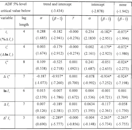
Table 3.1 ADF Regression CPI series September 1948 to September 1997: 63
Various Estimators
Table 3.2 ADF Regression for the rate of inflation: Various Time Periods 65
Table 3.3 PP Test CPI series September 1948 to September 1997: Various 66
Estimators
Table 3.4 PP Test for the rate of inflation: Various Time Periods 67
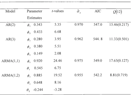
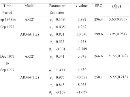
Table 3.5 ARMA Models, Fitting and Diagnostic Checking: Series /, 69
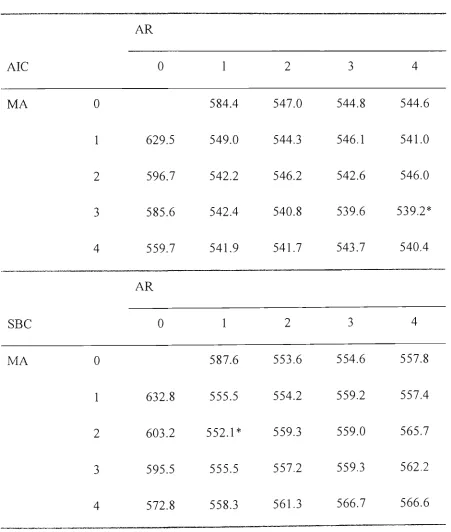
Table 3.6 Values of the AIC and SBC criteria for Different ARMA(p,q) 71
Models for the Rate of Inflation series: September 1948 to
September 1997
Table 3.7 ARMA Models, Fitting and Diagnostic Checking: Series i, with 73
a Break Point of September 1973
Table 3.8 ARMA Models, Fitting and Diagnostic Checking: Series 75
/; = Aln/,
Table 3.9 Values of the SBC criterion for Different GARCH(p,q) Models 83
for the Variance with the Mean Modelled as an AR(2) for the
Rate of Inflation series: September 1948 to September 1997
Table 3.10 AR(2)-ARCH/GARCH Models Diagnostic Testing 84
Table 3.11 AR(2)-GARCH(1,3) Parameter Values for the Whole Period and 85
Applying a Break Point at September 1973
Table 3.12 ADF Regression: Actual, Unexpected and Expected Inflation 89
series: March 1973 to September 1997
Table 3.13 PP Test Actual, Unexpected and Expected Inflation series: March 90
1973 to September 1997
Table 3.14 ARMA Models, Fitting and Diagnostic Checking: Series u, 92
Table 3.15 ARMA Models, Fitting and Diagnostic Checking: Series 94
Table 4.1 Relative Importance of Industrial and Mining Shares 1948 to 1969 102
Table 4.2 Adjustments to Extend the 10-year Treasury Bond Series to 105
March 1960.
Table 4.3 ADF Regression Equity series September 1948 to September 109
Table 4.4
Table 4.5
Table 4.6
Table 4.7
Table 4.8
Table 4.9
Table 4.10
Table 4.11
Table 4.12
Table 4.13
Table 4.14
Table 4.15
Table 4.16
Table 5.1
Table 5.2
Table 5.3
Table 5.4
Table 5.5
Table 5.6
PP Test Equity series September 1948 to September 1997 110
ARMA Models, Fitting and Diagnostic Checking: Series >^, 114
ARMA Models, Fitting and Diagnostic Checking: Series Iny, 115
ARMA Models, Fitting and Diagnostic Checking: Series Ad, 118
Preferred ARCH/GARCH Equity Models Diagnostic Testing 121
Preferred ARCH/GARCH Equity Models Parameter Values 122
ADF Regression Fixed Interest series March 1960 to September 127
1997
PP Test Fixed Interest series March 1960 to September 1997 128
ARMA Models, Fitting and Diagnostic Checking: Series m, 130
ARMA Models, Fitting and Diagnostic Checking: Series Ab, 132
ARMA Models, Fitting and Diagnostic Checking: Series An, 135
Preferred ARCH/GARCH Fixed Interest Models Diagnostic 136
Testing
Preferred ARCH/GARCH Fixed Interest Models Parameter 137
Values
Cointegration between Nominal Series: Tests Applied to the 145
Residuals from the Cointegrating Regression. Various Lengths of
Time Period
Log Likelihood Function and LR Statistic for Various Lag 147
Lengths in the Johansen Cointegration Test VAR. Nominal
Bonds and Nominal T-notes.
Johansen Cointegration Test: That the Hypothesised Number of 148
Cointegration Equations is None. Time Periods as in Table 5.1
Cointegration between Real Series: Tests Applied to the 150
Residuals fi-om the Cointegrating Regression. Various Length of
Time Period
Johansen Cointegration Test: That the Hypothesised Number of 151
Cointegration Equations is None. Time Periods as in Table 5.4
LR Statistic for Various Lag Lengths in the Johansen 152
Table 5.7 Unit Root Tests for hiflation and Share Prices 1875 to 1947. 154
Table 5.8 Summary Comtegration Statistics between Inflation and Share 155
Prices 1875 to 1947 and 1948 to 1997
Table 5.9 Johansen Cointegration Test: Trace test LR Statistics for /?,, b, 156
and d, . March 1960 to September 1997.
Table 5.10 Summary Cointegration Statistics between b,, p, and d,: June 157
1975 to September 1997
Table 5.11 ADF Regression 'Confidence' series: period maximum of 158
available data set
Table 5.12 PP Test 'Confidence' series: period maximum of available data 159
set
Table 5.13 Johansen Cointegration Test: Trace test LR Statistics for InP,, 160
hiB, and InD,. March 1960 to September 1997.
Table 5.14 Johansen Cointegration Test: Trace test LR Statistics for 162
AI,,p,,b,,n, and d, . March 1960 to September 1997.
Table 6.1 Correlations coefficients between z, and Financial Variables: 172
Time Period Maximum of the Available Data
Table 6.2 ADL(5,5):Regression of the Dividend Yield on Inflation 185
Table 6.3 Multicollinearity Diagnostics: Regression Table 6.2, rows 1 and 2 186
Table 6.4 ADL(5,5):Regression of the Real Dividend on Inflation 187
Table 6.5 ADL(5,5):Regression of the Real All Ordinaries on Inflation 188
Table 6.6 ADL(5,5):Regression of the Long/Short Ratio on Inflation 189
Table 6.7 ADL(5,5):Regression of the Real Bond Yield on hiflation 190
Table 6.8 Multicollinearity Diagnostics: Regression Table 6.7, rows 1 and 2 191
Table 6.9 ADL(5,5):Regression of the Real Treasury Note Yield on 193
Inflation
Table 6.10 Multicollinearity Diagnostics: Regression Table 6.9, rows 1 and 2 194
Table 6.11 ADL(5,5):Regression of the Real Variables on Unexpected 202
Inflation
Table 6.12 Multicollinearity Diagnostics: Regression Table 6.11, rows 7 and 203
Table 6.13 Multicollinearity Diagnostics: Regression Table 6.11, rows 9 and 203
10.
Table 6.14 Summary of Modelling Results with Three Altemative 205
Approaches
Table 7.1 Model Fit for Various Values of or in Regression (7.8) 227
Table 7.2 Non-Negativity Test: Annual Inflation Rates used in Model 229
(7.10) Simulation
Table 7.3 SBC Criterion and LR Statistic for Various Lag Lengths in the 233
Johansen Cointegration Test VAR. Real Bonds and Real T-notes.
Table 8.1 Correlation Matrix Between Stochastic Equation Error Terms for 257
the Period June 1975 to September 1997
Table 8.2 Correlations Between Selected Error Terms for Different Time 258
Periods
Table 9.1 Ex post Risk Premia December 1977 to April 1997 270
Table 9.2 Dividend yield Grossing Up Factors for the Franking Benefit by 273
Tax Rate and Average Franking Level
Table 10.1 Forecasts of Equity Indicators 289
Table 10.2 Forecasts of Fixed Interest Indicators 290
Table 10.3 Inflation Scenarios: Annual Rate of Inflation for the Next 10 291
Years
Table 10.4 Simulation Scenarios 1 to 5: Average Annual Nominal Returns 292
List of Figures page
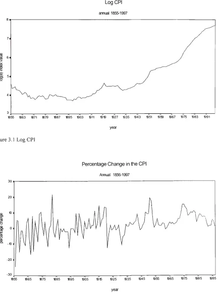
Figure 3.1 Log CPI 49
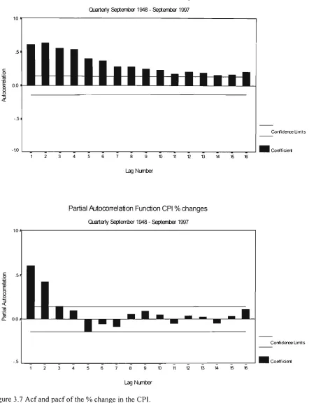
Figure 3.2 % change in the CPI, 49
Figure 3.3 10-year Rolling Estimator of the Variance of the % Change in 50
the CPI.
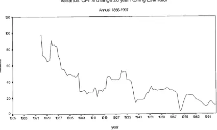
Figure 3.4 20-year Rolling Estimator of the Variance of the % Change in 50
the CPI.
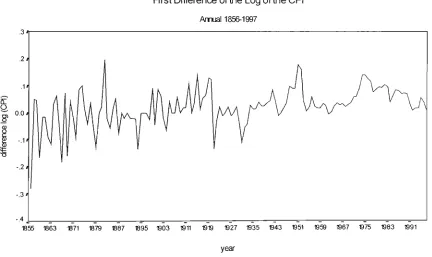
Figure 3.5 First Differences of the Log of the CPI. 52
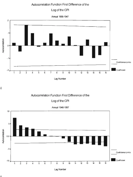
Figure 3.6 (a) and (b) Acf for the First Differences of the Log of the CPI 54
with a Stmctural Break at 1947.
Figure 3.7 Acf and pacf of the % change in the CPI. 68
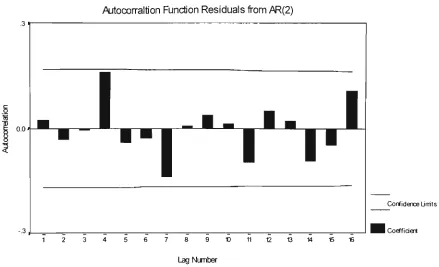
Figure 3.8 Acf of the Residuals fi-om Fitting an AR(2) Model to the % 74
change in CPI.
Figure 3.9 Acf and pacf for the Annualised CPI. 76
Figure 3.10 Median Value of Inflationary Expectations versus the 87
Annualised % change in the CPI.
Figure 3.11 Unexpected Inflation: Actual Inflation less Inflationary 88
Expectations.
Figure 4.1 Ratio of All Ords Dividend Yield to the Unweighted Dividend 100
Yield.
Figure 4.2 Ratio of All Ords Dividend Yield to the All Industrials Dividend 101
Yield.
Figure 4.3 Ratio of All Industrials Dividend Yield to the Unweighted 102
Dividend Yield.
Figure 4.4 The Dividend Yield on Ordinary Shares. 108
Figure 4.5 Acf and Pacf for equity series (a), {h)y,; (c), {d)Ad, and (e), 113
{f)Ap,.
Figure 4.6 Real Dividends on Ordinary Shares, the Nominal Dividend Index 116
Deflated by the CPI.
Figure 4.7 Real All Ordinaries Index: the Nominal All Ordinaries Index 119
Figure 4.8 Long /Short Ratio a Measure of the Spread in the Yield Curve 126
Between 10-year Treasury Bonds and Treasury Notes.
Figure 4.9 Acf and Pacf for fixed interest series (a), (b) m,; (c), (d) A b, and 129
{e),{f)An,.
Figure 4.10 Real 10-year Treasury Bond Rates, Nominal YTM of Treasury 131
Bond Deflated by Annualised Rate of Inflation.
Figure 4.11 Real Treasury Note Rates, Nominal Yield of Treasury Note 133
Deflated by Annualised Rate of Inflation.
Figure 5.1 Log of the All Ordinaries Index versus the log of the CPI from 153
1875-1975.
Figure 5.2 Ratio of the Bond Yield to the Dividend Yield or 'Confidence'. 160
Figure 6.1 Ccf for equity series: {ajy,; {h)Ad, and {c)Ap, and for fixed 173
interest series: (d) m,; (e) A b, and (f) A «,.
Figure 6.2 Recursive least squares coefficients of inflation (a) at lag 0 and 192
(b) at lag 4.
Figure 6.3 Recursive least squares coefficients of infiation (a) at lag 0 and 195
(b) at lag 4.
Figure 6.4 Transfer Function Model for Ab,: Ccf between the transformed 197
input and output series a, and fi,.
Figure 6.5 c^fs for pre-whitened equity series: (a);^, ; {h)Ad, and 200
{c)Ap, and for pre-whitened fixed interest series: (d) m, ;
( e ) A ^ / and {f)An, , where T represents the pre-whitening
transform.
Figure 7.1 Effectiveness of the Real Bond Model (6.4). 219
Figure 7.2 Yields on Indexed Bonds. 221
Figure 7.3 Volatility of the Difference in Real 10-year Treasury bonds using 222
a 20-quarter Rolling Estimator of the Variance.
Figure 7.4 Scatter diagram of the 20-quarter Rolling Estimator of the 223
Variance of the Difference in Real 10-year Treasury Bonds
Figure 7.5 Real and Nominal Bond Rates from a Simulation of the Real 229
Bond Model (7.10) using Inflation Rates from Table 7.2.
Figure 7.6 Real Bonds Versus Real T-Notes Showing Cointegration. 232
Figure 7.7 Impulse Response in An, Due to One Standard Deviation 236
Innovations in A n, and Ab,.
Figure 8.1 Impulse Response of Ap, Due to One standard Deviation 252
Innovations inAp, and Ad,.
Figure 8.2 Ccfs for the period June 1975 to September 1997 for the 254
Response to A b, of (a) y, and (b) A d, and to m, of (c) y, and
(d) Ad,.
Figure 9.1 Equity Risk Premium: Ex post Value of Equity Returns less 10- 270
year Treasury Bonds on a Rolling 12-month Returns Basis.
Figure 9.2 Equity Risk Premium (ERP): Ex c(«?e Value of Equity Returns 274
less 10-year Treasury Bond Returns Adjusted at the 50% and
100% Average Level of Franking for the Imputation Benefit Post
July 1987.
Figure 10.1 Schematic Diagram of the Proposed Model Stmcttire. 282
Figure 10.2 Comparison of Cumulative Difference in Returns between Using 288
Chapter 1
Introduction
1.1 Background
The discipline of financial reserving or the setting aside of reserves to meet fiiture
liabilities is central to a wide range of activities. Life insurance, superannuation and
long-tailed classes of general insurance are activities which fall into this class and are
typically long term in nature. Insurance contracts and the determination of
superannuation benefits depend upon having a level of assets available to meet long
term contractual liabilities. Since assets and liabilities are stochastic variables when
they are matched an appropriate level of risk is required. This is often given as the
probability of not meeting some target. In the case of an insurance company a typical
target would be the solvency ratio.' There is a statutory requirement that the solvency
ratio should exceed a certain level which is laid down by regulatory authorities as a
pmdential standard. Thus to write more business upon which to generate more profit
an insurer will normally have to raise more capital. This would normally be in the
form of equity.
The financial reserving process is about making financial estimates. Historically this
work has been the domain of actuaries. Traditional methods involve discounting
future liabilities with appropriate discount factors and matching these against
available assets. Hence solvency ratios can be determined. Following Markowitz and
the introduction of portfolio theory more detailed analyses of assets utilising these
principles have entered business practice. Past data on asset classes is collected and a
wide range of statistics calculated. These are then put together to form an efficient
frontier comprising asset mixes formed in an optimal manner. The efficient frontier is
a plot of the set of points yielding the best possible return for a given level of risk with
the given asset classes where risk is defined as the standard deviation of returns to the
portfolio of assets. Portfolio optimisation packages based upon quadratic
programming are now readily available.
Implicit in the production of financial estimates is the assumption of stability in the
mean level of asset class returns. The variance of returns is also assumed constant as
are the correlations between returns to asset classes. In the Markowitz method there is
no attempt to explain, for example, the values of the correlation coefficients between
returns to asset classes. If the random walk hypothesis^ with respect to share prices is
tme then attempts to predict ex ante returns to equity by other models will be
impossible. Increasingly however evidence has emerged to suggest a degree of
predictability in asset prices for both the fixed interest and equity markets. If this is so
then the returns to the particular asset class can be found. So with the help of models
projections can be made.
The finance literature now contains many studies detailing the predictability of asset
prices and in particular the concept of mean reversion. Mean reversion is the idea that
although returns to asset classes can wander away from a long mn mean level,
economic forces eventually take over and bring the mean level of retums back to a
long run level. There is an extensive literature on mean reversion with no complete
agreement either on its existence or extent. Nevertheless many in the finance industry
take mean reversion as a given and use valuation models to decide whether or not a
particular asset class is over or under valued relative to other asset classes.
The term stochastic investment model is extensively detailed in the Wilkie model, see
Wilkie (1984, 1987, 1992, 1995a and 1995b), which consisted of a series of stochastic
equations. The stochastic investment model is a multi 'asset class' model composed of
single asset class models. Each single asset class model is assumed to be described by
a number oi factors. In fixed interest, for example, a "parallel shift" factor is the
movement up or down along the whole yield curve. This factor can be captured by a
financial variable such as the long bond rate.
The financial variables can be modelled by stochastic equations. There are potential
connections or links within an asset class between individual stochastic equations.
The links may be a variable or coefficient that is shared by two or more stochastic
equations. The link may be between the random error terms in two or more stochastic
equations. For example, in fixed interest it may be hypothesised that the random error
term in any stochastic equation for the short term interest rate is linked to the random
error term in any stochastic equation for the long term interest rate. If the hypothesis is
correct then simulations should mirror this link.
There are potential links between asset classes through individual stochastic
equations. In a similar manner to the potential links within an asset class, links may be
made between the elements of the stochastic equations describing the different asset
classes. An example could be a potential link between long term bond rates and the
dividend yield. Wilkie postulates a number of such links between his stochastic
equations.
Individual stochastic equations modelling share or bond prices and respective rates of
return have been proposed in the literature. By applying a detailed analysis to a given
time series the underlying data generating process (DGP) of that series are modelled.
New econometric techniques have been developed which, in conjunction with the
increase in computing power, means that complex models can be developed and
intensive simulations on these models can be easily conducted. As a result there is a
wide range of competing models that are based upon stochastic equations within a
single asset class. Further, as the models become more complex in order to fit a given
data set, new evidence fi-om a new data set can quickly contradict the more complex
model.
There are however few stochastic investment models available in the public domain.
The essential 'facts' as to the stochastic equations and links between the equations are
different between competing models. There are also differences with the choice and
application of exogenous variables. In the Wilkie stochastic investment model the rate
of inflation is a driving force. The rate of inflation is modelled as a stochastic process.
the variables discounted by the CPI. This is the approach followed in the stochastic
investment model in this thesis and is a feature differentiating it from competing
models.
There are advantages of a stochastic investment system of real rather than nominal
variables. Firstly it is not essential to model the rate of inflation. If a satisfactory
model is available it can be applied. In practice the rate of inflation has proven
difficult to model. Otherwise future annual rates of inflation can be assumed as a
scenario. Thus a high or low inflation outlook can be considered. The stochastic
investment system can then be applied to generate retums under each different
scenario. Any changes in the rate of inflation under each scenario would therefore
cascade through the model system. Probabilities could be assigned to various
scenarios thereby generating a weighted average set of retums.
Secondly the scenario approach gives the ability to directly determine the impact of
changes in the rate of inflation. For superannuation tmstees or others responsible for
meeting long term liabilities, there is a desire to understand what would happen to
their particular portfolio if the financial environment, as defined by the inflation
outlook, were substantially different from that originally envisaged.
Another feature of the approach to the stochastic investment system proposed is
simplicity. Complex mathematical models may not be readily accepted by many of
those in positions of authority. Superannuation trustees cannot be expected to accept
something which they do not understand. Actuarial consultants have to communicate
what they propose and their reasons. Hence not only can one question the statistical
value of more complex models, but also whether they are useful tools for an actuary or
adviser.
Finally a brief comment on the econometric methodology is warranted at this stage.
The philosophy adopted is a pragmatic one consistent with the approach of Hendry et
al. at the London School of Economics. They are less concerned with how one finds a
model, rather the real test is whether the model stands up to scrutiny against
exogenous variables are introduced. Data analysis and univariate modelling, which
can be viewed as part of data analysis are conducted in Chapters 3-5.
1.2 Aims of the Document
Funds need to be managed and tmstees amongst others need advice as to how to
undertake the process of setting asset allocations. Methods to determine reserve
estimates and to aid in the decision making process such as a stochastic investment
model should therefore be targeted at the needs of the client. The stochastic
investment model needs to be easily understandable, flexible and capable of dealing
with the kinds of questions that decision makers must answer, such as the solvency
ratio for an insurance company or the probability of negative return for an industry
superannuation fund.
An aim of the thesis is to devise an appropriate stochastic investment model and apply
it. However to do so requires much background work. The design of a model requires
a close examination of the base data and a detailed investigation of the stmcture of the
financial series. It is necessary to reconcile existing research on financial markets.
Hence a primary aim of the thesis is to place the stochastic investment model in
context; what can be achieved is investigated. The predictability of asset prices for
financial reserving is examined in the context of stochastic investment model
development.
In developing the model potential relationships between asset classes will be
examined. The risk premia or extra compensation for being in one particular more
risky asset class over another will be investigated; in particular the equity risk
premium, the premium obtained from investing in equities rather than long term
bonds. In order to limit the scope of the thesis only the three asset classes of cash,
bonds and equities^ are considered. Property and intemational investments are not
covered. These latter asset classes can be added at a later stage. Hence an objective is
modularity in the stochastic investment model, whereby asset classes may be simply
added or subtracted.
It is important that the model is used for projections under various scenarios. To see a
model operate under various scenarios shows how useful it can be, for example, in
performing asset allocations. The resuhs obtained should be sensible. A range of
potential scenarios of the rate of inflation may be considered, then returns can be
compared and the level of the risk premium evaluated.
1.3 Outline of the Document
The plan to achieve the above aims is outlined in this section. There are some general
comments to be made about the document stmcture. Inflation, covered in chapter 3, is
central to actuarial estimates. If a satisfactory model of inflation can be found then it
may be applied and estimates made. However the model is one of real variables and
so modelling inflation as a stochastic process is not an essential requirement.
Scenarios generate inflation outlooks. Chapters 4-8 develop the model in a sequential
fashion. Thus each step refers back to previous results and conclusions. The chapters
nevertheless have a degree of independence each dealing with a separate feature of
model development. Chapter 9 is not central to the final stochastic investment model.
The equity risk premium, covered in chapter 9, is of prime importance to the cost of
capital and asset allocation. It is an output of the model and not a key step in model
development. Each chapter has a similar stmcture with an introduction, literature
review, exposition of theory, analysis and results followed by a summary and
conclusions. An overview of each chapter in the thesis now follows.
Chapter 2 reviews the literature. It summarises the literature and places the study in
the context of the overarching finance literature.
Chapter 3 covers inflation modelling. The first section introduces the inflation data
series and discusses the sources of information and any shortcomings. The Consumer
Price Index (CPI) is reviewed in the second section and measures of the mean level
and volatility of the CPI are considered. In the third section these are then explored for
stationarity via unit root testing. Univariate modelling is applied to the data utilising
standard Box-Jenkins methodology. In the fourth section some aspects of potential
heteroskedasticity are also investigated with the introduction of a range of non-linear
models. Various statistical measures generated fiom these processes will help to
understand the nature of the time series. The final section investigates inflationary
expectations and the role of unexpected inflation in financial market action. A model
of inflationary expectations is then developed.
Chapter 4 covers data analysis and univariate modelling of equities and fixed interest.
The first section details the data sources for the financial series used in the model and
any limitations. The second section considers the equity series. Unit root tests are
conducted to determine the order of integration of the financial variables. A series of
univariate models with stationary data are then developed to describe the DGPs. Then
heteroskedasticity and the normality of the residuals are considered with the
application of non-linear models. The third section performs the same task using the
fixed interest series. In so doing an understanding is gained of the common features in
the series.
In chapter 5 the inter-relationships between inflation, equities and fixed interest are
investigated within a cointegration framework. Hence long run relationships between
the integrated series can be assessed. In the first section concepts and definitions are
introduced. The Engle-Granger two-step procedure is used in the data analysis. The
Johansen maximum likelihood test is applied as a check on the procedure. In the
second section the set of real and nominal bivariate relationships is tested. The link
between inflation and nominal share prices is examined in the third section with a
long annual data series. In the fourth section the trivariate relationship between the
bond yield and the components of the dividend yield is investigated for both nominal
and real cases. In the final section all the real variables are considered together.
Chapter 6 covers the modelling of the stationary series with inflation as an exogenous
variable. The first section deals with issues in model building, reviewing some of the
relationship between inflation and each financial series. The chosen model form, from
the wide class of models available and the diagnostic tool kit are then reviewed. In the
third section this is applied to modelling the financial time series with the introduction
of inflation as an explanatory variable. Box-Jenkins transfer functions are used in the
fourth section. This provides an altemative approach to the standard linear regression
techniques. Unexpected inflation is then introduced as the independent variable in the
fifth section. The aim is to determine the role of expectations and to compare the
results with those obtained from using observed inflation. If unexpected inflation
provides superior results then the results of Chapter 3 can be applied to obtain
unexpected inflation from observed inflation. The chapter is concluded with a
discussion in the last section of the best equations for the stationary components in
the stochastic investment model. A comparison of results with the use of qualitative
judgments as well as the available diagnostics is made.
Chapter 7 covers the levels modelling of the integrated series for the fixed interest
asset class. The first section reviews some of the literature, the competing models and
the progress of research in Australia. In the second section an empirical analysis is
conducted which results in a real bond model which satisfies the requirements of
non-negativity and mean reversion. The third section covers the relationship between real
bonds and real T-notes. The number of factors needed to adequately model interest
rates and the yield curve is examined. The cointegrating relationship between real
bond rates and real T-note rates is utilised to enable the introduction of error
correction models (ECM) involving the levels of the two variables. The results of this
analysis can then be compared to the forecasting ability of the long/short ratio, which
is another way of viewing the cointegrating relationship. However the ratio does not
contain the extra information available in the levels data. Thus the question as to
whether a better model can be obtained from this extra data is considered.
Chapter 8 covers the levels modelling of the integrated series for the equities asset
class and any potential links between the non-stationary or integrated components of
equities and fixed interest. It also covers any potential links between the stationary
components of equities and fixed interest. The first section reviews some of the
long mn links between inflation, dividends and share prices, with levels data. An
ECM connecting real share prices and real dividends is found and compared to the
dividend yield model. The third section reviews connections between the differenced
stationary components of the series. Any potential links between the residuals from
the final equations are then reviewed to complete the investigation. The final section
reviews the stochastic investment model in the light of findings to present the working
model.
Chapter 9 introduces the equity risk premium (ERP). In the first section the concepts,
some definitions and the literature are reviewed. In the second section a methodology
for dealing with ex ante values is proposed. The value of the ERP is then adjusted for
dividend imputation and an assessment of the reasonableness of the current level is
performed. Future trends are then reviewed to see what range of values the ERP could
take. In the final section a potential modelling process for the risk premium is
outlined. A model of inflation expectations employing the cost of capital is put
forward. The model has significant limitations but has the potential for further
development. This provides a direct method of obtaining retums to shares via bond
returns.
Chapter 10 summarises the stochastic investment model providing out-of-sample
forecasts and scenario based simulations. The first section provides a schematic
overview of the model and the logic behind scenario building. Then in the second
section mechanisms are introduced to convert the stochastic model equations into
retums. The third section provides a set of forecasts which can be compared to actual
retums. There are available out-of-sample values for the period December 1997 to
September 1999. Scenarios are then set and simulations performed yielding sets of
asset class retums. The section is rounded off with a discussion of the shortcomings
and weaknesses of the model and some potential applications. The chapter concludes
with a discussion of the model.
Chapter 11 then concludes the thesis. The first section reviews the main findings. In
the second section these findings are then discussed in terms of any unresolved issues
The final section considers some potential directions that stochastic investment
modelling may take.
Finally, there is the caveat that care needs to be taken in moving between real and
nominal variables; yields to maturity or discount rates and retums; ex ante and ex post
retums. Much of the disagreement in the literature arises from differing definitions,
differing time periods for data analysis or results from different counfries with
Chapter 2
Survey of the Literature
2.1 Introduction
Financial reserving, as discussed in section 1.1, is an essential process for ensuring
financial security. The meeting of financial obligations ensures the future welfare of
both corporations and individuals. Hence the methodology for estimating financial
assets and liabilities is an extremely important business decision. Actuaries employ
different techniques to arrive at reserve estimates. These methods suppose a degree of
predictability in the assets and liabilities. The methods are often simple involving
assumptions about trends in asset returns and liabilities with appropriate asset
allocations and discount factors to find a NPV. A more formal method for determining
asset allocation is the Markowitz mean-variance technique, a single stage quadratic
programme. The Markowitz approach has been extended to liabilities with the
introduction of the concept of value at risk. The development of the techniques in the
actuarial profession continues. Stochastic investment models as outlined in section 1.1
are in the process of development to accommodate the perceived shortcomings of the
Markowitz method.
The aim of the literature review is to provide the scope of research in the arena of
stochastic investment modelling. As indicated in section 1.3 each chapter covers
literature pertinent to the issues under consideration in each chapter and is a more
comprehensive review. The literature review in chapter 2 puts the research in context.
The literature review breaks down into seven sections. In the first three sections
2.2-2.4 a review is conducted of the predictability of asset prices in the finance literature.
The review covers a wide range of topics. In section 2.5 multi-asset class models are
reviewed. These are termed stochastic investment models in this document, as
possible approaches to model building are discussed. Economefric methodology is
explored. Section 2.8 considers statistical issues. This section details techniques of
data analysis, econometric modelling and statistical inference, stochastic processes.
and recent advances in financial economics. It covers more general statistical
problems as well as specific issues faced in the analysis of financial data.
2.2 Asset Class Relationships and Predictability: US and International Experience
Research into anomalies in asset retums can be categorised in many different ways.
Broad categories could include asset predictors, both short and long run; mean
reversion and excess volatility; and a time varying risk premium. In this section
studies are categorised in order to capture the main directions of research both
internationally and in Australia.
2.2.1 Early Studies, Market Efficiency
The search for predictability in asset returns has a long history. The random walk
hypothesis and the efficient markets hypothesis (EMH) goes back to Bachelier (1900).
He proposed that the distribution of price changes were independent identically
distributed normal variables. Not until 1939 in the aftermath of the Great Depression
did the next important review, the Cowles Commission in the US, occur. The
intervention of WWII meant that research interest in asset price predictability
recommenced in the 1950's.
Kendall (1953) considered the autocorrelation stmcture of various financial time
series and concluded they were random walks. One exception he found to the random
walk hypothesis was a cotton price series where he had used averages. This inspired
the brief note from Working (1960), who showed that first differences of averages in a
The collection by Cootner (1964) contains a series of papers whereby various authors'
conducted a range of tests on series, in an attempt to see whether various frading mles
could be applied to "beat the markef. Fama (1970) in his review of financial markets,
pulled together some of the results of earlier research, to provide his definitions of
forms of market efficiency. The net result was that share prices were considered a
random walk.
Research since then has challenged the notion that asset prices are a random walk
process . A comprehensive review of speculative prices in the finance literature was
published by Fama (1991) revisiting his 1970 paper. It shows both the scope of the
field and the enormous growth in interest and research conducted since 1970. In this
later work Fama is less sure about the efficiency of markets. He cites many examples
of the predictability of share prices.
2.2.2 Cross Sectional Studies: Asset Predictors
A variety of papers have investigated potential predictors of asset prices, the list in
this sub-section is but a small sample; the results favour predictability. Keim and
Stambough (1986) sought ex ante variables with which to predict ex post risk premia.
They concluded that the level of asset prices contained information about expected
premiums, especially for the bond portfolios.
Fama and French (1989) investigated the relationship between expected returns and
general business conditions. They looked at certain defining characteristics of
business conditions and their relationship to the default spread, term spread and
dividend yield. Fama and French (1992) considered the predictability of cross
sectional returns. They found that average stock retums were not positively related to
the stock beta, a central tenet of the Sharpe-Lintner-Black model^. However they
concluded that for the 1963-1990 period, size and book-to-market equity captured the
cross sectional variation in average stock retums. These two predictors were
sufficient, explaining other predictor such as the earnings yield. Fama (1995) looked
at specific practice in stock markets, notably technical and fundamental analysis. This
short paper is aimed at the practitioner. Fama finds too little connection between the
academic and the practitioner. He feels that much market practice has little merit;
share market analysts need to expose their predictions to the ultimate test of
demonstrating a track record.
Hawawini and Keim (1995) reviewed the global evidence on the predictability of
stock retums. The authors investigated the application of forecasting variables such as
the term structure and dividend yield, noting that the recent research supported the use
of these and related variables to predict stock retums. The survey of a wide range of
empirical studies showed predictabilty in various facets of stock retums.
Zhou (1995, 1996) considered various models of share retums. Zhou (1996) assessed
the predictability of returns from the share market based upon the term stmcture. The
author claimed that there was a strong link between ex ante interest rates and expected
share returns and his single measure of the term stmcture.
2.2.3 Asset Returns and Inflation
The previous sub-section reviewed a small portion of the literature on general
predictabilty. The focus now moves to specific links between asset retums and
inflation.
Fama and Schwert (1977) considered the link between asset returns and the rate of
inflation. They found retums to bills, bonds and real estate to vary with their
definition of expected inflation, but stock retums to respond negatively and therefore
not to be a hedge against inflation. They concluded that the risk premium on stocks,
which they defined as the difference between the expected retums on stocks and bills,
was negatively correlated with the interest rate.
Lee (1992) found that interest rates explained a substantial fraction of the variation in
inflation and that inflation responded negatively to shocks in real interest rates. Lee
also found that inflation and stock retums were negatively correlated. He concluded
that stock retums explained much of the changes in real activity. However Campbell
and Ammer (1993) suggested a positive relationship between inflation and stock
retums. They pointed out the difference between a long mn and a short run effect. In
the long run stocks are a hedge against inflation. This proposition was tested by
Boudoukh and Richardson (1993) who conducted an empirical analysis of the
relationship between stock retums and inflation, based upon annual US data for
1802-1990 and UK data for 1820-1988. The authors concluded that strong support was
provided for a positive relation between nominal stock returns and inflation at long
horizons. They pointed out that to the extent that researchers developed theories to
explain the negative correlation at short horizons, these models should also be
consistent with their evidence.
In terms of the importance of potential predictors Golob and Bishop (1996) concluded
that stock prices follow inflation more closely than they followed interest rates. Any
link with long term interest rates was minimal, beyond that which was contained
through inflation and its effect in turn on interest rates. This potential link was
reviewed in Graham (1996) with an investigation into the causality of the negative
relationship between share retums and inflation, and the role that monetary policy
plays. This investigated Fama's conjecture that the link between inflation and stock
returns is in turn due to their common link to real activity. He concluded that the
negative relationship appears to arise only in periods when monetary policy is either
neutral or counter cyclical and when variability in the inflation rate is associated with
variability in the growth of real output.
Rather than inflation driving interest rates Lahiri and Dasgupta (1991) applied interest
indicators. They concluded by suggesting that the utility of a composite leading
indicator of inflation can be greatiy enhanced if price forecasts obtained from the bond
market are included as one of its components.
2.2.4 Excess Volatility and Mean Reversion
The concepts of excess volatility and mean reversion discussed in this sub-section are
introduced. These anomalies in finance have generated much debate in the literature.
Shiller (1979) considered the expectations model of the term stmcture of interest
rates. The expectations model implies that long term rates are a long term average of
short term rates plus the liquidity risk premium. Shiller demonstrated that any model
based on expectations cannot have the degree of volatility actually observed in long
rates, hence ipso facto the expectations model is incorrect. Shiller applied the same
technique to share prices. Campbell and Shiller (1988), Shiller (1989) found that share
prices exhibit 'excess volatility' that is movements in share prices are far greater than
that implied by the NPV model of dividends. In Campbell and Shiller (1988) excess
volatility is connected to the predictability of share prices via various factors such as
the dividend yield. The excess volatility observed is the basis of the predictability of
prices.
West (1988) reviewed the excess volatility debate and the associated 'bubbles'
literature. There are firstly statistical issues of inference. There is a small sample bias
caused by near unit roots. West finds that correcting the situation with tests
accounting for unit roots improves the situation but still leaves excess volatility.
Explanations for the excess volatility involve "rational bubbles"; alternative models of
retums or "fads" models. West reviews bubbles but rejects them as a potential
explanation. He looks at variations in expected retums but finds that traditional
models do not provide an explanation either. As regards fads he finds that there is
little formal positive evidence pertaining to fads models to sway someone
unsympathetic to fads models. West feels that non-constant expected retums are a
non-constant expected retums have manifested themselves in a variety of ways, the
difficulty is the source of the non-constant expected retums.
The mean reversion hypothesis (see section 1.1 for a discussion) was tested by Poterba
and Summers (1988). They applied the variance ratio'* test to U.S. stock prices and
found mean reverting behaviour. They showed that there is initially positive
autocorrelation in stock prices followed by negative correlation at longer lags. The
degree of this negative autocorrelation is small at any given longer lag but
accumulates to a significant total. Fama and French (1988a, 1988b) in two separate
papers looked at mean reversion and found similar resuhs; though the extent of mean
reversion in the long mn was dependent on the inclusion of the 1930's period. Lo and
McKinlay (1988) concluded that although stock prices were not a random walk, they
were also not described as a random walk plus a transient, mean reverting component.
Kim, Nelson and Startz (1998) revisited the Poterba and Summers resuhs by applying
a different sampling procedure to generate a sampling distribution for the variance
ratio statistic which differed from that of Poterba and Summers. They therefore
generated different /'-values to those obtained by Poterba and Summers and found
results which substantially weakened the evidence in favour of mean reversion.
De Bondt and Thaler (1989) reviewed mean reversion, event studies and the
predictability of short term price movements via predictors such as P/E ratios. They
suggested that many players are not entirely rational. They were pessimistic about the
chances for success for traditional models in which all agents are assumed fully
rational. They suggested that models in which some agents have non-rational
expectations of future cash flows or have faulty risk perceptions may offer greater
promise.
2.2.5 Time Varying Risk Premia
A potential explanation of excess volatility is that the risk premium varies over time.
Keim and Stambough (1986) sought ex ante variables which predict ex post risk
premia. The third section of the paper considers predicting risk premia. Their
regressions indicated better predictability with the lower grade stock and bonds (on
the basis the more risky the specific stock or paper the more leveraged it is to the risk
premium). They concluded that there is evidence of time varying risk premia and that
the levels of asset pices contain information about expected premiums especially for
bond portfolios.
Benari (1990) suggested that there are various eras which are more or less favourable
to different asset classes. These eras may persist for a long time until eventually the
system corrects itself He outlined three periods 1966-72; 1973-82 and 1983-88. A
determining factor of these eras was the nature of price inflation. The first period can
be characterised as one of stable but rising inflation. The second as accelerating
inflation and the third as declining inflation. Different types of asset did well under
each scenario. This view is consistent with Bollerslev and Hodrick (1995). The
authors summarised the key issues in finance and the econometric tests and estimation
procedures that have been applied to these topics, and concluded in favour of time
varying risk premia or eras in financial markets.
A similar conclusion was reached by Kurz and Beltratti (1996) and Kurz (1997), who
hypothesised that endogenous uncertainty is dominant in the equity market. There are
eras in the stock market when significant amounts of money, in real terms, could have
been lost. They extended these ideas to a theory of rational beliefs which they claimed
explains many of the anomalies in the finance literature. Chow and Ming (1997)
approach the excess volatility debate from the viewpoint of different eras or regimes.
The authors took a simple two state regime of dividend growth rates, those of
expansion and contraction. Thus hypothesising that the timing activity of investors
generated the observed excess volatility. They then defined their
expansion/contraction models, conducted simulations and showed 'excess volatility'
2.3 Asset Class Relationships and Predictability: Australian Experience
This next section reviews the literature on the issues discussed in section 2.2 in an
Australian context. Volker (1982) applied inflationary expectations and other potential
explanatory variables to model the Treasury bill rate. He concluded that for the period
1968-1979, liquidity conditions have been the major determinant of short term interest
rates in Australia and that inflationary expectations have been reflected to a significant
but relatively small degree.
Inder and Silvapulle (1993) discussed the Fisher effect for bank accepted bills. They
find that a 1% rise in inflation leads to a 0.5% rise in interest rates and hence a fall in
the real rate of 0.5%. Interest rates show stickiness, even in the long mn, with nominal
interest rates not responding fully to rises and falls in the inflation rate. Mishkin and
Simon (1995) examined the Fisher effect for T-notes. They tested the idea that a rise
in short term rates implied a rise in expected inflation rather than a tightening of
monetary policy. The authors concluded by finding that changes in short term interest
rates can reflect the stance of monetary policy. However in the long run it is changes
in inflation that affect the level of interest rates. Olekalns (1996) tested a less
demanding relationship, that of a partial adjustment of the expected inflation rate,
rather than the nominal interest rate fully incorporating anticipated changes in the
price level. He concluded that the nominal interest rate only partially adjusted to
anticipated inflation. However for the post-deregulation period alone analysis showed
that complete adjustment was achieved.
A series of Australian actuarially based papers were published in the 1990's. Carter
(1991) found no causal link between inflation and the All Ords index. The index was
best modelled as a random walk. He also found that interest rates were not a
significant determinant of the All Ords index. Fitzherbert (1992) found against
inflation as the long run determinant of the All Ords index. He maintained that
retained profits^ plus a partial adjustment for inflation, determined the long run trend
in share prices. This view is consistent with Graham, Dodd and Cottle (1962). Harris
(1994) concluded there was a positive relationship between quarterly real GDP growth
and quarterly All Ords index retums. He also found that there is a connection between
T-notes and All Ords index monthly retums but none between inflation and All Ords
index monthly retums.
Groenewald, O'Rourke and Thomas (1997) found a negative relationship between
stock retums and inflation. They did not find that monetary poHcy, either pro or
counter cyclical, has an impact. They concluded that the negative relationship between
stock retums and inflation was the outcome of interactions in the economy as a whole.
Inflation rates affected many macro variables some of which in tum, affected stock
returns in addition to any direct effect. Crosby (1998) found that a 1% positive shock
to inflation lead to a 0.1%) positive increase in the share index. The negative link
between stock prices and inflation is a short mn and not a long mn feature of the data.
2.4 Asset Class Relativities and the Equity Risk Premium
From individual asset predictability, the predictability of asset class relativities
follows. This naturally leads to tactical asset allocation (TAA) in funds management,
see Hodges (1995). Hence the attempt to build models to time movements between
asset classes. This leads to a measure of asset class return relativities and the concept
of the equity risk premium.
The ex post ERP has been determined by various authors in different markets. It is
noteworthy that only a few Anglo-Saxon markets can provide long term studies. In the
US Ambatscheer (1989) puts forward a risk premium of 2.5% over bonds and 4%
over T-bills. Siegel (1992) conducted a US sttidy over the period 1802-1990 and
found a steady level of the premium over short term bonds of 6%). Hathaway (1995)
for Australia found a post war arithmetic average equity premium over T-notes of
6.6%). Hibbard (1998) examined the New Zealand experience. He defined the ERP as
the excess return on equity over investment in a 90-day New Zealand Treasury bill.
He found that for the period September 1982 to December 1997 the value of the
average ERP was 6.2%. This is consistent with the Australian result. These results
The Australian results included no benefit for dividend imputation introduced in
Australia in July 1987. Officer (1992) believes that the effect of imputation should be
included in the premium either through the calculation of the rate of return, by
including the grossed up dividends or by making an adjustment to the normal CAPM
equation to include the value of the tax credits. This view is consistent with that of
Davis (1999) who argued for the full inclusion of the value of the franking credit.
Obtaining the ex ante ERP is harder. Clothier (1989) used an IRR as the expected rate
of return. Harris and Marston (1992) used analysts forecasts and the DDM to derive
the equity return for the US market over the period 1982-91. The ex ante ERP found
by Harris and Marston is similar to the long term average ex post ERP at
approximately 6%. Blanchard (1993) used annuity values to find real retums for the
variables under question. He found that the Great Depression of the !930's had
distorted the long term results. He concluded that the equity premium had gone down
steadily since the early 1950's. Infiation had contributed to the transitory increase
above trend in the 1970's and the transitory decrease below trend in the 1980's.
Yamaguchi (1994) defined the required risk premium as the excess return for equity
over bond yield demanded by an investor tolerant of a specific level of downside
probability. He deduced that prices in 1994 argued for a holding of greater than
normal weight in bonds.
Mehra and Prescott (1985) found a 'premium puzzle', caused by the size of the ex
post ERP. They defined the ERP as the return from the market over the return from
the riskless asset and found that k was too large relative to the level of the return from
the riskless asset. Hibbard (1998) found in favour of a similar 'puzzle' occurring in
New Zealand. Kurz and Beltratti (1996) and Kurz (1997) attempted to explain the
'premium puzzle' of Mehra and Prescott. They outiined a theory of Rational Belief
Equilibrium. The observations in financial markets are often the result of mistakes or
incorrect assessments. For example, making judgements based upon the norms for a
previous era when circumstances change. It takes time for participants to catch up
with the changes. If behefs and financial eras dominate then there will be periods of
consensus views and non-consensus views. Consequently in a strategic sense the
Then either trends are followed or upon the realisation that there has been a change of
state, assets are adjusted to the new era.
Papers from a meeting of academics and practitioners to discuss the ERP were
collected in the compendium by Sharpe and Sherred (1989). A problem with
generalisations is the conflicting definitions, data fransformations and analytical
methods employed. However even allowing for this there would appear to be
significant differences of opinion both with respect to the fact of predictability and the
potential causes.
French (1989) considered risk premia, defined as the return on the particular portfolio
minus the T-bill rate, with respect to various fundamental indicators such as the
dividend yield, the default spread and the term spread. He found evidence of the
predictability of the premium using these factors. Summers (1989) found that markets
consist of much noise but a long run tendency to revert to fundamental value. This
predictability of prices based upon fundamental indicators argues for mean reversion
strategies at times and momentum based strategies at other times. Sharpe (1989)
accepted mean reversion and then aimed to explain variations in the risk premium
with a wealth based proxy. On the other hand Nelson (1989) found problems with
mean reversion post-war, since the effect of the Great Depression of the !930's
overstated the issue. He argued that regression results found to date were due to
sample bias, accounting for much of the R' found in resuhs. The data to be really
conclusive was lacking.
Practitioners were more concerned with TAA and appropriate models. Clothier (1989)
described the system in place at Wells Fargo. The IRR is used as a proxy for the
expected rate of return and the risk premia between the respective asset markets is
used as the indicator in TAA. He claimed excellent results with this approach.
Henriksson (1989) (Kidder Peabody) followed a similar approach to Clothier. The
gains come from mean reversion and from doing the opposite of what the majority of
the market does. Grossman (1989) described a system called informational TAA. The
model he described attempted to segment out the risk preference induced moves in
relativities. Brinson (1989) (Brinson & Associates) applied his analysis to the global
scene. He gave a table of values for risk premia, ranging from 5.6% for the UK to
4.6% for Japan. Brinson's method of determining risk premia is a process based on
both historical data and the understanding of the local market. He then applied TAA,
by using deviations from equilibrium at various levels, in a similar way to that
described by the other practioners.
A more behavioural approach to market dynamics is provided by Tversky (1989). He
outlined how people actually think about risk. He identified examples of 'irrational'
behaviour such as loss aversion; the segregation of individual assets (seeing the trees
not the wood); and the overconfidence inherent in estimates about the future when
actually tested.
Reichenstein and Rich (1993) assessed the predictability of stock retums with
predictors such as the earnings yield, dividend yield and the ERP. They found value in
the ERP and used it in TAA and indicated where it could add value. Finnerty and
Leistikow (1993) considered various risk premia and modelled the processes with a
mean reverting model, both with and without a trend component. The authors took the
period 1926-89 and found evidence of both mean reversion and a downtrend in the
ERP.
2.5 Stochastic Investment Models
A stochastic investment model is a multi-asset class model composed of stochastic
equations which represent the DGP of the factors that are sufficient to describe each
asset class as described in section 1.1.
There are few stochastic investment models. Stochastic investment models were
popularised by Wilkie (1984, 1987, 1992, 1995a and 1995b). The Wilkie approach
used inflation as a driver with expected inflation modelled as an exponentially
weighted moving average (EWMA) of observed inflation. Wilkie postulated that in
the long run inflation will be fully incorporated into the income stream of assets.
with lags. Wilkie included many links between predictive variables. For example the
random shock term from the dividend yield equation is a component in the equation
describing the yield on long term bonds. There is no justification given for the
stochastic equations and links between them, and these failings form the basis of
certain criticisms of the model.
As a public document Wilkie's model has been extensively reviewed. The paper by
Geoghegan et al (1992) resulted from a comprehensive report to the UK Institute of
Actuaries, authored by Harvey. The report reviewed the value and application of
stochastic models with particular reference to Wilkie's model. The report is in three
parts. The first outlined Wilkie's model, altemative models and the use of the Wilkie
model. The second part is a series of appendices which included an updated non-linear
inflation model and the consideration of ARCH^ effects in the series. The last three
sections of the second part investigated the application of the model in aspects of
actuarial work, such as pension funds, life offices and investment management. The
third part is a discussion by participants and others of various topics raised by the
report as well as more general issues. The discussion included; the inflation model
(negative rates of inflation, ARCH effects); the use and modification of the model by
life offices; and technical issues such as parameter estimates, the number of
simulations and the extent of actuarial judgement.
Other actuaries have seen a role for such modelling^. TPF&C^ (Mulvey and
Vladimirou 1992, Mulvey 1994,1996, Mulvey and Ziemba 1995 and Mulvey and
Thoriacius 1997) have directiy funded research. The CAPLINK model of TPF&C is a
cascade structured model, see Mulvey (1994) for a description. Mulvey made certain
assumptions such as stock returns were dependent upon a number of factors including
the economic conditions of the companies, inflation, interest rates and momentum.
Whilst considerable detail is given, the TPF&C model is proprietary. For example, the
Engle (1982) introduced models with varying volatility or conditional heteroskedasticity as one method of dealing with heteroskedasticity. Engle applied this model to the UK inflation rate.
A recent model by Duval, Teeger and Yakoubov (1999) appeared whilst the model herein was being finalised. Stochastic investment models developed for Japan, South Afi-ica and Finland are also mentioned.