A Novel Parameter Estimation Method Based on LSU-EKF for Polynomial Phase Signal

A Novel Parameter Estimation Method Based on

LSU-EKF for Polynomial Phase Signal

Yi-xiong Zhang1,*, Hua-wei Xu1,†, Rong-rong Xu1,†, Zhen-miao Deng1,†and Cheng-Fu Yang2,*

1 _{Department of Communication Engineering, Xiamen University, Fujian 361005, China;}

hw.xu@rcstech.org (H.X.); dougonxu@gmail.com (R.X.); dzm_ddb@xmu.edu.cn (Z.D.)

2 _{Department of Chemical and Materials Engineering, National University of Kaohsiung, Kaohsiung, Taiwan}

* Correspondence: zyx@xmu.edu.cn (Y.Z.); cfyang@nuk.edu.tw (C.Y.); Tel.: 86-592-2965385 (Y.Z.);

00886-7591-9283 (C.Y.).

† These authors contributed equally to this work.

Abstract:The parameter estimation problem for polynomial phase signals (PPSs) arises in a number of fields, including radar, sonar, biology, etc. In this paper, a fast algorithm of parameter estimation for monocomponent PPS is considered. We propose the so-called LSU-EKF estimator, which combines the least squares unwrapping (LSU) estimator and the extended Kalman filter (EKF). First, the coarse estimates of the parameters of PPS are obtained by the LSU estimator using a small number of samples. Subsequently, these coarse estimates are used to initial the EKF. Monte-Carlo simulations show that the computation complexity of the LSU-EKF estimator is much less than that of the LSU estimator, with little performance loss. Similar to the LSU estimator, the proposed algorithm is able to work over the entire identifiable region. Moreover, in the EKF stage, the accurate estimated results can be output point-by-point, which is useful in real applications.

Keywords:radar; polynomial phase signal; least squares unwrapping; extended Kalman filter

1. Introduction

Parameter estimation of Polynomial phase signals (PPSs) are common in many fields, including radar, sonar, geophysics, radio communication and biology [1–3]. In radio communication, continuous-phase signals are used to generate signals with attractive spectral efficiency [4,5]. The parameter estimation for PPSs is well indicated for the underwater monitoring of vessels and marine fauna [6,7]. It is known that frequency modulated (FM) signals are frequently used in radar and sonar [8], where the phase shift caused by the relative target motion can be modeled as a continuous function of time. In radar applications, the performance of target detection and motion compensation can be significantly improved by using the a priori knowledge of motion parameters. Therefore, precise estimations of range, velocity, and acceleration obtained from the echoes of high-speed targets, such as rockets and missiles, are of great importance for radar detection and imaging [9,10]. In recent years, parameter estimation of PPS has attracted considerable attention and many methods have been proposed [11–25]. Among these methods, a typical estimator of the unknown coefficients is the least squares estimator [11,12], which is an effective approach, being both computationally efficient and statistically accurate when the noise is white and Gaussian. However, this method becomes extremely complex for PPS with second and higher orders.

To estimate the parameters of higher-order PPS, researchers have developed more efficient methods based on “multilinear transforms” or “phase unwrapping”. Examples of multilinear transform techniques include the cubic phase function (CPF) [13,14], the high order ambiguity function (HAF) [15,16] and the product HAF (PHAF) [17], which have good performance with less computational complexity, and can be adapted to process multicomponent signals. Nevertheless, for the HAF-based approaches, the phase differentiation (PD) is used to decrease the order of PPSs, which increases the number of noise terms. As a result, each PD increases the SNR threshold and the MSE. Another drawback of the HAF-based approach and the CPF estimator, is that the region

of coefficients searched by these estimators is much smaller than the size of the identifiable region. One of the alternative methods is phase unwrapping (PU), which utilizes the fact that the phase of a complex sinusoid is a linear function which is wrapped into (0, 2π). A classical estimator based on PU is the least squares unwrapping estimator (LSU) [18,19]. The significant advantage of this approach is that it works for PPS contained anywhere inside the identifiable region. The estimator also appears to perform well when the low signal-to-noise ratio (SNR) threshold is reached. The major drawback of the LSU estimator is that, in general, computing a nearest lattice point leads to a large computational cost. Especially, the algorithm becomes prohibitively complex when the number of samples is larger than 1000 [19].

The parameter estimation by using the extended Kalman filter (EKF) has been investigated in the case of PPS affected by Gaussian noise [20]. A disadvantage is that the convergence of EKF depends strongly on the initial values. In this paper, a novel method which combines the LSU estimator and the EKF is proposed. A small number of initial samples are used to estimate the parameters of PPS. Then these coarse estimates are used to initiate the EKF. Meanwhile, a theoretical derivation is conducted on the proper number of samples used in the initialization step. Numerical simulations show that the proposed method can work with low SNR threshold and exhibit high performance with small computational complexity. Moreover, this method is accurate over a much wider range of parameters than other state-of-the-art existing estimators.

The rest of this paper is organized as follows: The signal model is presented in Section 2 and the LSU estimator in introduced in Section 3. Then, the state-space representation of PPS, and the EKF based parameter estimation algorithm are introduced in Section 4. In Section 5, the proper number of samples used in the initialization phase is investigated, and the arithmetic complexity of the proposed method is analyzed. To validate the effectiveness and advantages of the proposed algorithm, Monte-Carlo simulations are conducted in Section 6. Finally, conclusions are given in Section 7.

2. Signal Model

The received PPS can be written as

y(n) =Ae2πjθ(n)_{+w(n) (1)}

whereAis the signal amplitude, andw(n)denotes the complex additive white Gaussian noise (AWGN), with mean zero and varianceσ2.θ(n)is a polynomial of orderm, which is expressed by

θ(n) =u0+u1n+u2n2+· · ·+umnm (2)

whereui, i=0, . . . ,m, are real-valued and unknown coefficients, and their identifiable regions are

written as [26]

− 1

2i! ≤ui< 1

2i!, i=0, 1, 2,· · ·,m. (3) 3. The Least Squares Unwrapping Estimator

The LSU estimator attempts to estimate the coefficients by performing linear regression on the phase of received signal. The angle ofy(n), denoted6 _{y(n), is written as}

6 _{y(n) =2πθn =2π(φn+θ(n))(mod2ß) (4)}

whereφnis a random variable representing the phase noise induced byw(n), and it can be calculated

as [28]

φn =

6 ₁₊ w(n)

Ae2πjθ(n)

According to the fundamental of least square method, the parameters u0, u1, ..., um can be

evaluated by

SS(u) =argmin

∑

n=1

θn−

∑

2

(6)

whereNrepresents the number of samples.

Due to the phase ambiguity in6 _{y(n), we may define}

D

θn−

∑

E

=θn−

∑

wherebxcdenotes the nearest integer tox. By consideringbϕnc=

j

θn−∑m_k=0uknk

k

as a nuisance parameters,SScan be rewritten as

SS(u) =argmin

∑

n=1

D

θn−

∑

E2

. (8)

The LSU estimator is the minimizer ofSS(u)over the identifiable region, which can be represented as a nearest lattice point problem [29]. When the number of samples is less than 60, the sphere decoder [30] can exactly compute a nearest lattice point. On the other hand, if the number of samples is larger than 60, another approximate nearest point algorithm called the K-best algorithm [31] is applied, which requiresO(N3logN)operations. As a result, the LSU estimator needs much more operations as the number of samples, i.e.,Nincreases.

According to the asymptotic normality and strong consistency of LSU estimator [18,19], the mean square error (MSE) of this estimator can be obtained by

MSE= Psignal

2h1− f−1 2

i2 10SNR10

·D−1./G (9)

wherePsignaldenotes the power of the polynomial phase signal, f(·)is the probability density function

ofφnandA./Bmeans element-by-element division between matrixAand matrixB. The superscript

-1 denotes the inverse operator. MatrixDis am+1 bym+1 Hilbert matrix with elements

Di,j=1/(i+j+1), i,j∈[0, 1, 2,· · ·,m] (10)

and the matrixGcan be defined as

G=



    

N N2 · · · Nm+1 N2 _N3 _{· · · N}m+2

..

. ... . .. ... Nm+1 _Nm+2 _{· · · N}2m+1



    

. (11)

According to (9), more samples for the LSU estimator should be chosen to make the EKF work effectively at lower SNR. However, this will increase the computational cost conversely.

4. EKF based Parameter Estimation for PPSs

The state-space model associated with PPSs is described by two equations: the state transition equation and the observation equation:

Xn =FnXn−1+υn−1 Yn =h(Xn) +ωn

whereXnis the discrete-time state vector andYnis the observation vector,υn−1represents the state

noise vector andωnis the vector of noise in the measured signal.

4.1. The Observation Equation

Since the signal (1) is complex, it is necessary to express the measured signal as a 2×1 vector in terms of its real and imaginary part

Yn=Re(y(n)) Im(y(n))T. (13)

In this sense, the observation equation takes the form

Yn=h(Xn) +ωn (14)

where the 2×1 nonlinear observation functionh(Xn)is written as

h(Xn) =

" h1n

h2n

# =

"

Acos(2πθ(n)) Asin(2πθ(n)) #

. (15)

The observation noise vector is defined asωn= [wR(n),wI(n) ]T, whose correlation matrixRnis given

by

Rn =



 

σ_ω2 2 0 0 σ 2 ω 2  

. (16)

In this paper, we assume that the process-noiseυnand the observation noiseωnare not correlated,

i.e.,

cov ωk,υj=EωkvTj

=0(k,j=0, 1, 2, 3,· · ·). (17) Consequently, the observation model of PPSs is nonlinear.

4.2. The State Transition Equation

The state-model of PPSs can be described by a set of continuous-time differential equations, that is,

dX(t)

dt =AX(t) +Lυ(t) (18) where the (m+1)×(m+1) constant matrix A and the (m+1)×m constant matrix L, which characterize the behavior of the model, are written as

A=           0 0 .. . 0 0 1 0 .. . 0 0 0 1 .. . 0 0 · · · · · · . .. · · · · · · 0 0 .. . 1 0 0 0 .. . 0 0          

,L=           0 1 0 .. . 0 0 0 1 .. . 0 · · · · · · · · · . .. · · · 0 0 0 .. . 1           (19)

andυ(t)is the process noise with a process noise matrixQc

Qc=Eυ(t)υT(t). (20)

Xn =θ(n) θ(1)(n) θ(2)(n) · · · θ(m)(n)T (21)

whereθ(m)(n)denotes themorder derivative ofθ(n). In order to use the discrete-time state (21), the model (18) must be discretized somehow [27], and can be described in the form

Xn =FnXn−1+υn−1 (22)

whereFnis the transition matrix of the dynamic model, which can be represented as

Fn=ϑ(Ts) =eATs = I+ATs+· · ·+

(ATs)k

k! +· · · (23)

whereTs is the step-size of the discretization. On the other hand,υn−1with varianceQn−1is the

discretized form ofυ(t)andQn−1satisfies

Qn−1= Z T_s

0 ϑ

(τ)LQcLTϑT(τ)d(τ). (24)

Therefore, the state-model of PPSs is linear.

4.3. Parameter Estimation of PPSs using EKF Algorithm

Since the observation model is nonlinear, we use the EKF algorithm to estimate the parameters of PPSs:

EKF Algorithm

Initial Conditions(n=0): ˆ

X0=E(X0) ˆ

P0=E h

(X0−Xˆ0)(X0−Xˆ0)

Ti (25)

Predict Equations:

X0n=FnXˆn−1

P0n =FnPˆn−1FTn+Qn−1 Y0_n= HnX0n

Hn=

δh δX _X0

n

(26)

Update Equations:

Kn =P0nHTn·

h

HnP0nHTn+Rn

i−1 ˆ

Xn =X0n+KnYn−Y0n

ˆ

Pn = [I−KnHn]P0n

(27)

The relationship between the parametersui, i=0,· · ·,m, of PPSs and the initial state vectorX0

is described by

u=CX0 (28)

where the matrixCis defined as

C=diag

1 1 1 2! · · ·

1 m!

Therefore, the parameters of PPSs is estimated in the form

ˆ u=C×

n

∏

i=1

F−_i 1 !

×_Xˆ_{n. (30)}

Using a Taylor series based transformation, the EKF extends the scope of Kalman filter to nonlinear optimal filtering problems by forming a Gaussian approximation to the joint distribution of stateXand measurementsY. In this sense, the EKF is sensitive to the initial conditions. If the filter is improperly initialized, the filter may fail. In this paper, in order to make the filter work effectively, we utilize the estimated results of the LSU estimator to initialize the EKF. Considering the computational cost of the LSU estimator, only a few samples are used to obtain the initial estimates.

5. Performance Analysis of The Proposed Method

As the convergence of EKF depends strongly on the initial values of coefficients, in the proposed LSU-EKF estimator, the LSU estimator is used to obtain the initial values for the EKF and make the filter work effectively. As described above, the computational cost of LSU estimator increases significantly as the number of samples increases. In this section, we first discuss about the appropriate number of samples used in the initialization phase. Meanwhile, the computational complexity of the proposed method is analyzed.

5.1. The Number of Samples Used in The Initialization Phase

In order to obtain the appropriate number of samples used in the initialization phase, it is necessary to analyze the stability and convergence of the EKF. Due to the fact that the EKF equations are approximate nonlinear, it is difficult to conduct the convergence analysis for these systems. Many research have been conducted to deal with this problem [32–35]. In general, the sufficient conditions to ensure convergence of the EKF in this paper can be described as follows:

αn+1en+1=Hn+1X˜

0

n+1

˜

X0n+1=βnFnX˜n

(31)

where

˜

X0n+1=Xn+1−X0n+1

˜

Xn=Xn−Xˆn

en+1=Yn+1−Hn+1X0n+1

(32)

andαn+1∈R2·2,β_n ∈R(m+1)·(m+1)are unknown time-varying diagonal matrices, i.e.,

αn+1=diag{α1,n+1,α2,n+1} (33)

and

β_n =diag{β1,n,· · ·βm+1,n} (34)

which satisfy

αi,n+1∈ h

1−p

1−∆n+1, 1+ p

1−∆n+1 i

(i=1, 2) (35)

βj,n ∈[−1, 1] (j=1,· · ·,m+1) (36)

∆n+1=λmax(Rn+1)λmax

R−_n+1₁Hn+1P0nHnT+1

Hn+1P0nHTn+1+Rn+1 −1

(37)

whereλmax(∼)represents the maximum eigenvalue, and

Rn =

" σω2

2 0

0 σω2 2

#

(38)

P0=MSE×



      

1 1 2! · · · m! 1 1 2! · · · m! 2! 2! (2!)2 · · · 2!m!

..

. ... ... . .. ... m! m! 2!m! · · · (m!)2



      

. (39)

On the other hand, the state-space modelization of polynomial phase signals is linear, we can obtain

β_n =Im+1 (40)

Therefore, the appropriate number of samples used in the initialization phase can be obtained when satisfying (35).

5.2. Complexity Analysis

The main process of the EKF composes of two stages: prediction and updating. Assume that the discrete-time state vectorXnof PPSs is ani×1 vector and the observation vectorYnis aj×1 vector.

The arithmetic complexity of the proposed method can be derivated as follows.

The number of arithmetic operations of the predict equations (26) and the updating equations (27) are 2i3_+3i2_+ijandi3_+j3_+4ji2_+ij2_+i2_+j2_{+3ij+j+i, respectively. Thus, the number of}

arithmetic operations of the EKF is

T(i) =3i3+j3+4ji2+ij2+4i2+j2+4ij+j+i. (41) In the initialization process, the LSU estimator using the K-best algorithm [31] requires O(N13logN1)(N1means the number of samples used for the LSU estimator) arithmetic operations.

Denoting the number of arithmetic operations in the initialization process as TLSU, then the

computational complexity of the proposed algorithm is

T(N) =TLSU+T(i)·N (42)

This shows that the computational complexity of the proposed method isO(N). 6. Simulation

In this section, to find the minimum number of samples used in the initialization step, the proposed method is first evaluated with different number of initial samples. Then we compare the the performance of the proposed method with other existing estimator, in the cases of big and small coefficients, respectively. In each experiment, 2000 times of Monte Carlo simulations have been carried out.

6.1. Numerical Analysis on the Number of Samples in the Initialization Step

First, we conduct some simulations at different SNRs. When the SNR is 12 dB, and the number of samples used in the simulations is 499, the sample MSEs of the four coefficients(u0,u1,u2,u3)for

LSU-EKF estimator performs well when the number of initial samples is over 12. Considering the complexity of LSU estimator, the optimal number of initial samples for the LSU-EKF estimator is 12 when the SNR is 12 dB. In the same way, the optimal number of initial samples for PPSs of orderm=3 andm=4 as shown in Table1and Table2at different SNRs, respectively.

N

1

5 10 15 20 25 30 35 40 45 50

MSE u

0

10-4

10-3

10-2

LSU-EKF CRB

(a)

N

1

5 10 15 20 25 30 35 40 45 50

MSE u

1

10-8 10-7

10-6

10-5 10-4 10-3

10-2 LSU-EKF

CRB

(b)

N

1

5 10 15 20 25 30 35 40 45 50

MSE u

2

10-13 10-11 10-9

10-7

10-5

10-3 _LSU-EKF

CRB

(c)

N

1

5 10 15 20 25 30 35 40 45 50

MSE u

3

10-17

10-15

10-13

10-11

10-9 10-7 10-5

LSU-EKF CRB

(d)

Figure 1. Estimation for PPSs of order 3 by the LSU-EKF estimator with different initial samples. (a)MSE for the coefficientu0. (b)MSE for the coefficientu1. (c)MSE for the coefficientu2. (d)MSE for

the coefficientu3.

Table 1.The optimal number of samples used in the initialization phase at different SNRs for PPSs of order 3.

SN R(dB) 2 3 4 5 6 7 8 9 10 11 12 13 14 15

N1 225 155 143 93 64 43 31 25 24 17 12 11 9 8

Table 2.The optimal number of samples used in the initialization phase at different SNRs for PPSs of order 4.

SN R(dB) 9 11 13 15 17 19

6.2. Comparison with Other Existing Estimators

Then, the performances of the LSU estimator [18], the HAF estimator [16], the PHAF estimator [17], the Zhou and Wang (ZW) estimator [36] are compared with the proposed LSU-EKF estimator under the same experimental parameters. In practice, one would prefer to keep the number of samples used for the LSU estimator constant rather than changing the value with different conditions whether the optimal value is known or not. Here the number of samples used in the simulations is set to 199 and the number of initial samples used in our method is set to 64. The MSEs of the LSU estimator, the HAF estimator, the PHAF estimator, the ZW estimator, and the proposed estimator are shown in

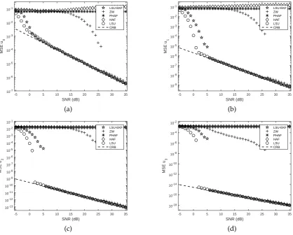
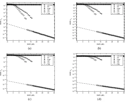
Fig.2and Fig.3, where the values of coefficients areu=h1₄,1₄,1₈,₂₄1,₉₆1,₄₈₀1 iTfor the 5-order PPSs and

u=h1₄,1₄,1₈,₂₄1iTfor the 3-order PPSs. The volume of the coefficients suitable for the HAF estimator, the PHAF estimator and the CPF estimator is much smaller than the identifiable region [14,15,17]. Hence, in this case, these estimators will fail. Alternatively, the ZW estimator can work on the entire identifiable region by extending the Euclidean algorithm, which comes with the cost of performance, including MSE and the threshold SNR.

SNR (dB)

-5 0 5 10 15 20 25 30 35

MSE u

0

10-7

10-6 10-5

10-4 10-3

10-2

10-1 LSU-EKF

ZW PHAF HAF LSU CRB

(a)

SNR (dB)

-5 0 5 10 15 20 25 30 35

MSE u

1

10-9

10-8

10-7 10-6

10-5

10-4

10-3 10-2

10-1

LSU-EKF ZW PHAF HAF LSU CRB

(b)

SNR (dB)

-5 0 5 10 15 20 25 30 35

MSE u

2

10-13 10-12

10-11

10-10 10-9 10-8 10-7 10-6 10-5

10-4

10-3 10-2 10-1

LSU-EKF ZW PHAF HAF LSU CRB

(c)

SNR (dB)

-5 0 5 10 15 20 25 30 35

MSE u

3

10-18

10-16

10-14 10-12 10-10

10-8

10-6 10-4 10-2

LSU-EKF ZW PHAF HAF LSU CRB

(d)

Figure 2.Performance comparison of different estimators for a polynomial phase signal of order 3 with

u=h1₄,1₄,1₈,₂₄1iTandN=199. (a) MSE for the coefficientu0. (b) MSE for the coefficientu1. (c) MSE

SNR (dB)

-5 0 5 10 15 20 25 30 35

MSE u 2 10-11 10-10 10-9 10-8 10-7 10-6 10-5 10-4 10-3

10-2 LSU-EKF

ZW PHAF HAF LSU CRB (a) SNR (dB)

-5 0 5 10 15 20 25 30 35

MSE u 3 10-15 10-14 10-13 10-12 10-11 10-10 10-9 10-8 10-7 10-6 10-5 10-4

10-3 LSU-EKF

ZW PHAF HAF LSU CRB (b) SNR (dB)

-5 0 5 10 15 20 25 30 35

MSE u 4 10-19 10-17 10-15 10-13 10-11 10-9 10-7 10-5 LSU-EKF ZW PHAF HAF LSU CRB (c) SNR (dB)

-5 0 5 10 15 20 25 30 35

MSE u 5 10-26 10-24 10-22 10-20 10-18 10-16 10-14 10-12 10-10 10-8 10-6 10-4 LSU-EKF ZW PHAF HAF LSU CRB (d)

Figure 3.Performance comparison of different estimators for a polynomial phase signal of order 3 with

u=h1₄,1₄,1₈,₂₄1,₉₆1,₄₈₀1 iT. (a) MSE for the coefficientu2. (b) MSE for the coefficientu3. (c) MSE for the

coefficientu4. (d) MSE for the coefficientu5.

The proposed LSU-EKF estimator can reach a threshold of 6 dB for the 3-order PPSs and of 17 dB for the 5-order PPSs. The corresponding threshold SNRs for the LSU estimator are 2 dB for the 3-order PPSs and 12 dB for the 5-order PPSs, respectively. The reason is that the number of samples used for the LSU estimator is larger than that for the LSU-EKF estimator in the initialization step. Table

3shows the time costs of all the estimators. It is seen that the computational complexity of the LSU estimator is approximately 24 times as much as that of the LSU-EKF estimator for the 3-order PPSs and 15 times for the 5-order PPSs. This simulation is performed on a high-performance computer with Intel(R) Core(TM) i5-4590 CPU 3.30 GHz and 8.0 GB of RAM. In fact, the SNR thresholds for the LSU-EKF estimator can be lower by using more samples for initialization, with increased time cost. Therefore, it is a tradeoff between the performance and the computational complexity.

Table 3.Time cost of different methods for PPSs of order 3 and PPSs of order 5. (in seconds)

HAF PHAF ZW LSU LSU-EKF

m=3 100.4s 180.5s 119.6s 25624.1s 1063.7s

m=5 114.3s 174.1s 177.4s 44883.4s 3113.7s

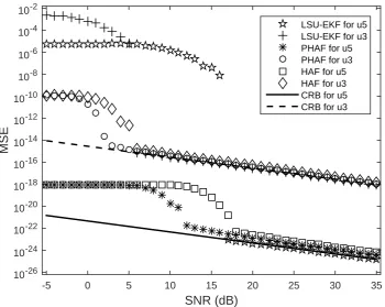
In order to make the values of the coefficients suitable for the HAF and PHAF estimator, we set the coefficients asu=h1₄,1₄,₈1_N,₂₄1_N2,₉₆1_N3,₄₈₀1_N4

iT

for the 5-order PPSs andu=h1₄,1₄,₈1_N,₂₄1_N2

the 3-order PPSs. In Fig.4, it can be seen that the HAF estimator reaches a threshold of 6 dB, which is the same as the proposed method for the 3-order PPSs. For the 5-order PPSs, the threshold of the HAF estimator is about 18 dB, slightly higher than that of the proposed method. Also, the PHAF estimator has a good performance on estimation of the coefficientsu3for the 3-order PPSs andu5for the 5-order

PPSs. As expected, the performance of the proposed method remains unchanged for the set of small coefficients.

SNR (dB)

-5 0 5 10 15 20 25 30 35

MSE

10-26

10-24

10-22

10-20

10-18

10-16

10-14

10-12

10-10

10-8

10-6

10-4

10-2

LSU-EKF for u5 LSU-EKF for u3 PHAF for u5 PHAF for u3 HAF for u5 HAF for u3 CRB for u5 CRB for u3

Figure 4.Performance comparison of different estimators for the coefficientu3for PPSs of order 3 with

u=h1₄,1₄,₈1_N,₂₄1_N2

iT

and the coefficientu5for PPSs of order 5 withu=

h

1

4,14,81N,241N2,₉₆1_N3,₄₈₀1_N4

iT

.

Pulse index

0 100 200 300 400 500 600 700 800 900 1000

Velocity estimation(m/s)

2385 2390 2395 2400 2405 2410 2415 2420

Real velocity LSU-EKF

(a)

Pulse index

0 100 200 300 400 500 600 700 800 900 1000

Velocity estimation bias(m/s)

-1.4 -1.2 -1 -0.8 -0.6 -0.4 -0.2 0 0.2

(b)

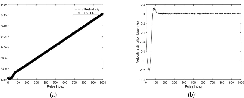
Figure 5. Velocity estimation for real radar data by the the LSU-EKF estimator. (a)Comparison of the estimated velocity and the real velocity. (b)The error between the estimated velocity and the real velocity.

7. Conclusion

In this paper, a novel parameter estimator based on LSU-EKF algorithm for PPSs is proposed. In the proposed LSU-EKF estimator, the coarse estimates of the parameters of PPS are first obtained by the LSU estimator using a small number of samples. Then, these coarse estimates are used to initial the EKF. Compared with the HAF-based approaches and the CPF estimator, the available region of coefficients of the proposed estimator is much larger. The simulation results demonstrate that the proposed method can work over entire identifiable region as the LSU estimator. The advantage of the LSU-EKF estimator is that its computational cost is much lower than the LSU estimator, with little performance loss. The threshold SNR of the LSU-EKF estimator is a bit higher than that of the LSU estimator, as less samples are used in the LSU stage of the LSU-EKF estimator. The number of samples to initial the EKF is relative to the threshold SNR and the computation complexity. Therefore, when using the proposed LSU-EKF estimator in real applications, the number of the initial samples should be carefully considered according to the tradeoff between these two factors.

Acknowledgments:The research was supported by the National High-tech R&D Program of China, the Open-End Fund National Laboratory of Automatic Target Recognition (ATR), the Open-End Fund of BITTT Key Laboratory of Space Object Measurement and the National Natural Science Foundation of China (Grant No. 62101196).

Author Contributions: Yi-xiong Zhang, Zhen-miao Deng and Cheng-Fu Yang conceived and designed the experiments; Hua-wei Xu performed the experiments; Rong-rong Xu analyzed the data; Hua-wei Xu and Cheng-Fu Yang contributed reagents/materials/analysis tools; Yi-xiong Zhang and Hua-wei Xu wrote the paper; Yi-xiong Zhang, Zhen-miao Deng and Cheng-Fu Yang modified the paper.

Conflicts of Interest: The authors declare that the grant, scholarship and/or funding mentioned in the Acknowledgments section do not lead to any conflict of interest. Additionally, the authors declare that there is no conflict of interest regarding the publication of this manuscript.

References

1. Xin, Yuan. Polynomial-phase signal source tracking using an electromagnetic vector-sensor.IEEE Conf. on

Acoustics, Speech and Signal Processing.2012,22, 2577–2580.

2. Zou, Y, X.; Li, B.; Ritz, C, H. Multi-Source DOA Estimation Using an Acoustic Vector Sensor Array Under a

Spatial Sparse Representation Framework. Circuits, Systems, and Signal Processing.2016,35, 993–1020.

3. Simeunovic, M.; Djurovic, I. Parameter Estimation of Multicomponent 2D Polynomial-Phase Signals Using

the 2D PHAF-Based Approach. IEEE Trans. Signal Processing.2016,64, 771–782.

4. Granados, O.; Andrian, J. Space-time block coding with symbol-wise decoding for polynomial phase

5. Shuai, Yao.; Shiliang, Fang.; Xiaoyan, Wang. Parameter estimation for hfm signals using combined stft and iteratively reweighted least squares linear fitting. Signal Processing.2014,99, 92–102.

6. Wang, K.; He, J.; and Shu, T. Joint angle and delay estimation for underwater acoustic multicarrier CDMA

systems using a vector sensor. IET Radar, Sonar and Navigation.2016,10, 774–783.

7. Gunes, A.; Guldogan, M, B. Joint underwater target detection and tracking with the Bernoulli filter using an acoustic vector sensor.Digital Signal Processing.2016,48, 246–258.

8. Anish, Turlapaty.; Yuanwei, Jin. Parameter estimation and waveform design for cognitive radar by minimal

free-energy principle. IEEE Conf. on Acoustics, Speech and Signal Processing.2013, 6244–6248.

9. Barbarossa, S.; Di Lorenzo, P.; Vecchiarelli, P. Parameter Estimation of 2D Multi-Component Polynomial

Phase Signals: An Application to SAR Imaging of Moving Targets. IEEE Trans. Signal Processing. 2014,

62, 4375–4389.

10. Yong, Wang.; Bin, Zhao.; Jian, Kang. Asymptotic Statistical Performance of Local Polynomial Wigner

Distribution for the Parameters Estimation of Cubic-Phase Signal With Application in ISAR Imaging of Ship Target. IEEE Journal. Selected Topics in Applied Earth Observations and Remote Sensing.2015,8, 1087–1098.

11. Djurovic, I.; Stankovic, L. Quasi-maximum-likelihood estimator of polynomial phase signals. IET Signal

Processing.2014,8, 347–359.

12. Francois, Vincent.; Olivier, Besson.; Eric, Chaumette. Approximate maximum likelihood estimation of two

closely spaced sources. Signal Processing.2014,97, 83–90.

13. Igor, Djurovic.; Pu, Wang.; and Cornel, Ioana. Parameter estimation of 2-d cubic phase signal using cubic

phase function with genetic algorithm.Signal Processing.2010,90, 2698–2707.

14. O’Shea, P. A fast algorithm for estimating the parameters of a quadratic FM signal. IEEE Trans. Signal

Processing.2004,52, pp. 385–393.

15. Peleg, S.; Friedlander.; Benjamin. vThe discrete polynomial-phase transform. IEEE Trans. Signal Processing. 1995,43, 1901–1914.

16. Cornel, Ioana.; Cedric, Cornu.; Andre, Quinquis. Polynomial phase signal processing via warped highorder

ambiguity function. IEEE Conf. on Signal Processing.2004, 1159–1162.

17. Sergio, Barbarossa.; Anna, Scaglione.; Georgios, B, Giannakis. Product high-order ambiguity function for

multicomponent polynomial-phase signal modeling. IEEE Trans. Signal Processing.1998,46, 691–708.

18. Robby, G, McKilliam.; Barry, G, Quinn.; Bill, Moran. Polynomial phase estimation by least squares phase

unwrapping. IEEE Trans. Signal Processing.2004,62, 1962–1975.

19. Robby, G, McKilliam.; Barry, G, Quinn.; Bill, Moran. Frequency estimation by phase unwrapping. IEEE

Trans. Signal Processing.2010,58, 2953–2963.

20. Peter, J, Kootsookos.; Joanna, Spanjaard. An extended kalman filter for demodulation of polynomial phase

signals.IEEE Signal Processing Letters.1998,5, 69–70.

21. Djurovic, I.; Simeunovic, M.; Djukanovic, S. A hybrid CPF-HAF estimation of polynomial-phase signals:

Detailed statistical analysis. IEEE Trans. Signal Processing.2012,60, 5010–5023.

22. Amar, A.; Leshem, A.; van, der, Veen, A.-J. A Low Complexity Blind Estimator of Narrowband Polynomial

Phase Signals. IEEE Trans. Signal Processing.2010,58, 4674–4683.

23. Peleg, S.; Friedlander.; Benjamin. A technique for estimating the parameters of multiple polynomial

phase signals. Time-Frequency and Time-Scale Analysis, Proceedings of the IEEE-SP International Symposium. 1992, 119–122.

24. Pu, Wang.; Hongbin, Li.; Himed, B. Instantaneous frequency estimation of polynomial phase signals using

local polynomial Wigner-Ville distribution. Proc. Int. Conf. Electromagnetics in Advanced Applications (ICEAA). 2010, 184–187.

25. Djurovic, I.; Simeunovic, M. Parameter estimation of non-uniform sampled polynomial-phase signals using

the HOCPF-WD.Signal Processing.2015,106, 253–258.

26. Robby, G, McKilliam. Identifiability and aliasing in polynomial-phase signals. IEEE Trans. Signal Processing. 2009,57, 4554–4557.

27. Zarchan, Paul.; Musoff, Howard. Fundamentals of kalman filtering: A practical approach; the American Institute of Aeronautics and Astronautics: Reston, VA, USA, 2005.

29. Erik, Agrell.; Thomas, Eriksson.; Alexander, Vardy. Closest point search in lattices.IEEE Trans. Information Theory.2002,48, 2201–2214.

30. Gianmarco, Romano.; Domenico, Ciuonzo.; Pierluigi, Salvo, Rossi. Low-complexity dominance-based

sphere decoder for mimo systems.Signal Processing.2013,93, 2500–2509.

31. Zhan, Guo.; Peter, Nilsson. Algorithm and implementation of the k-best sphere decoding for mimo detection.

IEEE Journal. Selected Areas in Communications.2006,24, 491–503.

32. Ljung, L. Asymptotic behavior of the extended Kalman filter as a parameter estimator for linear systems.

IEEE Trans. Automatic Control.1979,24, 36-50.

33. Song, Y.; Grizzle, J, M. The Extended Kalman Filter as a Local Asymptotic Observer for Nonlinear

Discrete-Time Systems. American Control Conference.1992,5, 3365-3369.

34. Moraal, P ,E.; Grizzle, J, M. Observer design for nonlinear systems with discrete-time measurements. IEEE

Trans. Automatic Control.1995,40, 395-404.

35. Boutayeb, M.; Rafaralahy, H.; Darouach, M. Convergence analysis of the extended Kalman filter used as an

observer for nonlinear deterministic discrete-time systems. IEEE Trans. Automatic Control.1997,42, 581–586.

36. G, Tong, Zhou.; Yang, Wang. Exploring lag diversity in the high-order ambiguity function for polynomial