i
Daily streamflow estimation using remote
sensing data
Meepegalkatiya Gamage Sisiri Danaka Nilantha
B. Sc. (Peradeniya), Postgrad-Dip. (Dehradun), M. Tech. (Visakpattnam)
Thesis submitted in fulfillment of the requirement for
the degree of Doctor of Philosophy
College of Engineering and Science
Victoria University
Australia
i
Dedicated to
my beloved wife - Ancy,
i
ABSTRACT
Streamflow data are critical for water resource investigations, and their development projects. However, the scarcity of such data, particularly measured streamflow through streamflow gauges, constitutes a serious impediment to the successful implementation of development projects. In the absence of such measured streamflow data, streamflow estimation using measured meteorological data represents a viable alternative. Nevertheless, this alternative is not always possible due to the unavailability of required meteorological data. In the face of such data limitations, many have advocated the use of remote sensing (RS) data to estimate streamflow. The aim of this study was to generate daily streamflow time series data using remote sensing data through catchment process modelling and statistical modelling.
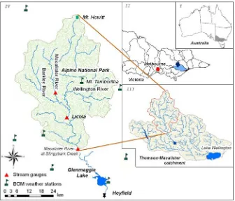
This study was conducted in two contrasting case study areas. The first case study area was the Macalister catchment in Australia, which is a data rich catchment. The second case study area was the Ribb catchment in Ethiopia, which is a data scarce catchment. The Soil and Water Assessment tool (SWAT) was used as the catchment process modelling tool, and Artificial Neural Networks (ANN) were used as the statistical modelling technique. Remote sensing data were used to estimate rainfall and potential evapotranspiration (PET), and to classify landuse/landcover (LULC), which in turn were used as inputs to catchment process modelling. Various vegetation and thermal indices, and brightness temperature were considered as surrogates to meteorological variables. They were used as inputs to statistical modelling to estimate daily streamflow.
ii
used as ground measured PET data. The results showed that the daily streamflow estimation with ground measured data was the best, while the daily streamflow estimation with estimated rainfall and estimated PET was the poorest. No significant difference to the daily streamflow estimates was noted when SWAT model derived PET was substituted with estimated PET.
For the Ribb catchment, the calibrated model parameters were used to estimate daily streamflow by replacing ground measured rainfall and SWAT model derived PET with estimated rainfall and estimated PET (both estimated from remote sensing data). Note that similar to the Macalister catchment ground measured data were not available for the Ribb catchment and therefore the SWAT derived PET data were used as ground measured PET data Intermediate models as used in the Macalister catchment were not considered in the Ribb catchment. This was because the model with ground measured rainfall data and estimated PET data produced similar results to the base model, and the model with estimated rainfall and SWAT model derived PET produced similar results to the model with estimated rainfall and estimated PET, in the Macalister catchment. The results of the base model were the best, and the results of model run with estimated rainfall and estimated PET is reasonable. This showed that estimated variables using remote sensing data can successfully be employed in catchment process modelling to estimate daily streamflow in both data rich and data scarce catchments at the same level of accuracy.
iii
Results also showed that the performance of ANN models with vegetation indices, thermal indices and brightness temperature in both case studies was better than the performance of the catchment process models with estimated rainfall and estimated PET (both estimated from remote sensing data). Furthermore, the results indicated that the performance of ANN models (i.e. seasonal) in both case studies were as good as the performance of the catchment process models (i.e. base models) developed with ground measured data.
iv
DECLARATION
I, Meepegalkatiya Gamage Sisiri Danaka Nilantha declare that the PhD thesis
entitled ‘Daily streamflow estimation using remote sensing data’ is no more than 100,000
words in length including quotes and exclusive of tables, figures, appendices, bibliography, references and footnotes.
This thesis contains no material that has been submitted previously, in whole or in part, for the award of any other academic degree or diploma. Except where otherwise indicated, this thesis is my own work.
………..
Meepegalkatiya Gamage Sisiri Danaka Nilantha
v
ACKNOWLEDGEMENTS
This PhD could not have been undertaken without the support of various people. Although it is not possible to give particular mention to all of them here, I gratefully acknowledge all their contributions.
Above all, I would like to express my heartfelt gratitude to my principal supervisor, Professor Chris Perera for his support, guidance and encouragements whilst giving me freedom to pursue independent work. I am very fortunate to have Professor Perera as my mentor. He not only dedicated significant time and efforts to review my work, but also introduced me to the right networks and kept me focused throughout this journey. I could not have asked for a better role model – knowledgeable, patient, compassionate and inspirational – and I hope I can make him proud in the future.
I am also deeply indebted to Dr. Vladimir Smakhtin, my associate supervisor, for his valuable comments and for encouraging me to undertake a PhD in the first place. His help in tackling administrative tasks at the International Water Management Institute (IWMI) and in introducing me to IWMI’s Ethiopian office staff ensured the smooth progression of my studies.
To the individuals and organisations who supported me during field work, I owe a huge debt of thanks. Particularly, I would like to thank the IWMI team at Colombo including Dr. Colin Charters, Dr. David Molden, Mr. David van Eyck, and Mr. Lal Muthuwatte; the IWMI Ethopian office including Dr. Matthew McCartney; and the Ethiopian Ministry of Water Resources and the Ethiopian National Meteorological Organisation.
vi
LIST OF PUBLICATIONS AND AWARDS
Journal Articles:
Gamage, N., Perera, C., 2014 Estimate streamflow data using Artificial Neural Network
models with remote sensing based vegetation and thermal indices. Journal of Hydrology (In submission)
Gamage, N., Smakhtin, V., Perera, C., 2014. Estimation of Potential Evapotranspiration using Remote Sensing Data for data scarce catchments. Remote Sensing of Environment. (Under review)
Conference Articles:
Gamage, N., Smakhtin, V., Perera, C., 2011. Estimation of Actual Evapotranspiration using Remote Sensing Data. In: Chan, F., Marinova, D., Anderssen, R.S. (Eds.), 19th International Congress on Modelling and Simulation. Modelling and Simulation Society of Australia and New Zealand, Perth Conventional and Exhibition Centre, pp. 3356-3362.
Gamage, N., Smakhtin, V., Perera, C., 2011. Simulating streamflow using remote sensing data: Artificial neural network approach, XXV IUGG General Assembly - Earth on the Edge: Science for a Sustainable Planet, Melbourne Convention and Exhibition Centre, Melbourne, Australia.
Gamage, N., Agrawal, R., Smakhtin, V., and Perera, B. J. C. (2011). An Artificial Neural Network Model for Simulating Streamflow Using Remote Sensing Data. In: 34th IAHR World Congress - Balance and Uncertainty, 26 June - 1 July (2011), Brisbane. Australia: IAHR & Engineers Australia, pp 1371 - 1378.
Awards:
• Finalist to Outstanding Student Award by Victoria University Alumni -2013. • Awarded travelling scholarships to attend international conferences.
vii
TABLE OF CONTENTS
ABSTRACT ... I DECLARATION ... IV ACKNOWLEDGEMENTS ... V LIST OF PUBLICATIONS AND AWARDS ... VI TABLE OF CONTENTS ... VII LIST OF FIGURES ... XIII LIST OF TABLES ... XVII LIST OF ABBREVIATIONS AND UNITS ... XIX
1
Chapter 1: Introduction ... 1-1
1.1 Stress on water resources ... 1-2 1.2 Importance of this investigation ... 1-4 1.3 Applications of remote sensing ... 1-7 1.4 Objectives of the study ... 1-9 1.5 Research methodology ... 1-10 1.6 Research significance ... 1-13 1.7 Outline of the thesis ... 1-13
2
Chapter 2: Streamflow estimation using remote sensing – A
critical review ... 2-1
viii
2.4.1.2 Rainfall estimation using remote sensing data ... 2-17 (a) Use of visible and thermal remote sensing data for rainfall estimation ... 2-17 (b) Use of microwave data for rainfall estimation ... 2-20 (c) Use of combined data for rainfall estimation ... 2-22 2.4.1.3 Evapotranspiration estimation using remote sensing data ... 2-22 2.4.1.4 Landuse/landcover classification ... 2-26 2.4.2 Use of statistical models ... 2-30 2.4.2.1 Artificial Neural Networks applications on streamflow estimation ... 2-33 2.4.2.2 Remote sensing based indices for streamflow estimation ... 2-35 2.5 Summary ... 2-38
3
Chapter 3: Study Area, data and methodology ... 3-1
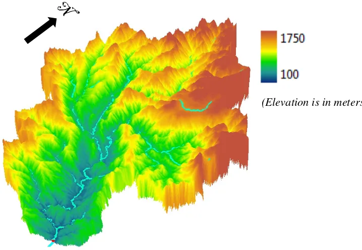
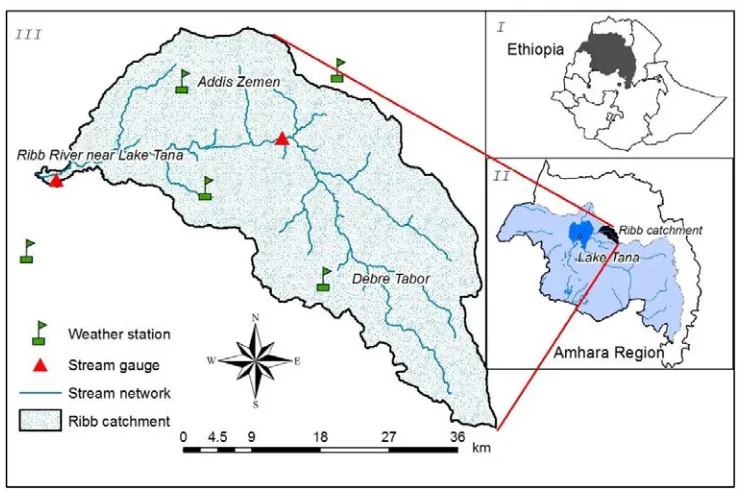
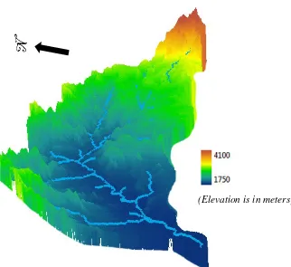
3.1 Introduction ... 3-1 3.2 Rationale for the selection of study areas ... 3-1 3.2.1 The first case study area ... 3-1 3.2.2 The second case study area ... 3-2 3.3 The Macalister catchment ... 3-5 3.3.1 Data ... 3-11 3.3.1.1 Remote sensing data (satellite-based data) ... 3-12 3.3.1.2 Ground-based data ... 3-14 3.4 The Ribb catchment ... 3-15 3.4.1 Data ... 3-22 3.4.1.1 Remote sensing data (satellite-based data) ... 3-22 3.4.1.2 Ground-based data ... 3-22 3.5 Estimation of input variables using remote sensing data for catchment process modelling ... 3-23
ix
3.5.2.2 Estimation of Rn24 for cloudy days ... 3-38
3.5.3 Classification of landuse/landcover ... 3-39 3.5.3.1 Ground-truth data collection ... 3-42 3.5.3.2 Training of satellite image ... 3-42 3.5.3.3 Classification stage ... 3-44 3.5.3.4 Accuracy assessment ... 3-44 3.6 Catchment process modelling ... 3-48 3.6.1 Brief description of SWAT ... 3-48 3.6.2 Model set up and calibration ... 3-50 3.7 Estimation of remote sensing based indices for statistical modelling ... 3-52 3.7.1 Selection of remote sensing based indices ... 3-52 3.7.2 Equations used to generate remote sensing based inputs for statistical modelling ... 3-53 3.8 Statistical modelling ... 3-55 3.8.1 Influential inputs ... 3-57 3.8.2 Artificial neural networks modelling ... 3-58 3.9 Performance assessment ... 3-63 3.10 Summary ... 3-64
4
Chapter 4: The Macalister catchment ... 4-1
x
4.2.3.1 Principal Component Analysis ... 4-25 4.2.3.2 Results of landuse/landcover classification ... 4-26 4.2.3.3 Accuracy assessment of the landuse/landcover classification ... 4-29 (a) Descriptive techniques ... 4-29 (b) Analytical techniques ... 4-33 4.3 Catchment process modelling ... 4-34 4.3.1 Model calibration and validation with ground measured data ... 4-36 4.3.2 Streamflow estimation with remote sensing based input variables ... 4-43 4.3.2.1 Model with estimated PET and ground measured rainfall ... 4-44 4.3.2.2 Model with estimated rainfall and SWAT derived PET ... 4-46 4.3.2.3 Model with estimated rainfall and estimated PET ... 4-50 4.3.2.4 Flow duration curves for all models ... 4-53 4.4 Streamflow estimation using statistical modelling ... 4-54 4.4.1 Remote sensing based input variables and streamflow ... 4-55 4.4.2 Determination of influential variables ... 4-61 4.4.3 Artificial Neural Networks modelling ... 4-64 4.4.3.1 Streamflow estimation - total period model ... 4-65 4.4.3.2 Streamflow estimation with seasonal ANN models ... 4-67 4.4.3.3 Performance assessment of ANN models ... 4-72 4.5 Comparison of catchment process modelling and statistical modelling ... 4-73 4.6 Summary ... 4-76
5
Chapter 5: The Ribb catchment ... 5-1
xi
5.2.2.2 PET of cloudy days ... 5-12 5.2.2.3 Mean annual PET ... 5-14 5.2.2.4 Performance of PET estimates for total period and seasons ... 5-14 5.2.3 Landuse/landcover classification ... 5-15 5.2.3.1 Principal Component Analysis ... 5-16 5.2.3.2 Results of landuse/landcover classification ... 5-17 5.2.3.3 Accuracy assessment of the landuse/landcover classification ... 5-19 (a) Descriptive technique ... 5-19 (b) Analytical technique ... 5-22 5.3 Catchment process modelling ... 5-23 5.3.1 Model calibration and validation using ground measured data... 5-24 5.3.2 Model with estimated rainfall and estimated PET ... 5-28 5.3.3 Comparison of results of base model and model with estimated rainfall and estimated PET ... 5-31 5.4 Streamflow estimation using statistical modelling ... 5-32 5.4.1 RS based input variables and streamflow ... 5-33 5.4.2 Determination of influential input variables ... 5-38 5.4.3 Artificial Neural Networks modelling ... 5-39 5.4.3.1 Streamflow estimation with seasonal ANN models ... 5-39 5.4.3.2 Performances of ANN based streamflow estimation ... 5-43 5.5 Comparison of results from catchment process modelling and statistical modelling ... 5-44 5.6 Summary ... 5-45
6
Chapter 6: Summary, conclusions and recommendations .... 6-1
xii
6.1.2.2 Determination of influential input variables ... 6-9 6.1.2.3 Artificial Neural Networks modelling ... 6-10 6.1.3 Comparison of catchment process modelling and statistical modelling ... 6-10 6.2 Conclusions ... 6-11 6.3 Limitations and directions for future research ... 6-12
7
References ... 7-1
xiii
LIST OF FIGURES
xiv
xv
xvi
Figure 5.12 Measured and estimated streamflow of the Ribb catchment – base model .. 5-26 Figure 5.13 Scatter plots of the measured and estimated streamflow of the Ribb catchment – base model ... 5-26 Figure 5.14 Scatter plots of the measured and estimated streamflow of wet and dry seasons in the Ribb catchment – base model ... 5-27 Figure 5.15 Measured streamflow, and estimated streamflow with both estimated rainfall and PET – Ribb catchment ... 5-29 Figure 5.16 Scatter plots of the measured and estimated streamflow of the Ribb catchment with both estimated rainfall and PET... 5-29 Figure 5.17 Scatter plots (seasonal) measured and estimated streamflow of the Ribb catchment – model with both estimated rainfall and PET ... 5-30 Figure 5.18 Flow duration curves of measured and estimated streamflows – Ribb catchment ... 5-32 Figure 5.19 Streamflow and 8-day average of EVI, NDWI and NDVI in the Ribb catchment ... 5-34 Figure 5.20 Streamflow and BT31 of MODIS in the Ribb catchment ... 5-36 Figure 5.21 BTdiff and streamflow in the Ribb catchment ... 5-36
Figure 5.22 BTgrad and streamflow in the Ribb catchment ... 5-37
xvii
LIST OF TABLES
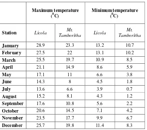
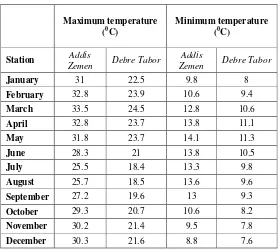
Table 2.1 Band widths and spatial resolution of the MODIS sensor ... 2-10 Table 3.1 Mean monthly maximum and minimum temperatures at Licola and Mt. Tamboritha ... 3-8 Table 3.2 Mean monthly maximum and minimum temperatures at two different meteorological stations over the Ribb catchment ... 3-18 Table 3.3 Contingency matrix of the rain/no-rain combinations of MODIS BT and TRMM ... 3-29 Table 3.4 Landuse/landcover classes ... 3-41 Table 4.1 Mean seasonal BT and mean monthly BT over the Macalister catchment ... 4-5 Table 4.2 HSS, POD, FAR and bias values for the different thresholds – Macalister catchment ... 4-6 Table 4.3 Rain/no-rain days under TRMM and estimated rainfalls during the study period ... 4-13 Table 4.4 Comparison of surface albedo of the Macalister catchment ... 4-15 Table 4.5 Estimated and PM based mean annual PET-Macalister catchment ... 4-21 Table 4.6 Performance indices of estimated PET and PM based PET - Macalister catchment ... 4-23 Table 4.7 Band information of the Landsat 5 TM sensor ... 4-25 Table 4.8 Areas of the catchment covered by different LULC classes (after image classification) ... 4-29 Table 4.9 Contingency matrix of the landuse/landcover classification – the Macalister catchment ... 4-31 Table 4.10 Kappa statistics and user’s accuracy of the landuse/landcover classification 4-34 Table 4.11 SWAT model parameters used for calibration purposes ... 4-38 Table 4.12 RMSE (in Ml/day) and Ef values of the streamflow estimation using measured
xviii
Table 4.16 Performance indices of the estimated streamflow from various ANN models – Macalister catchment ... 4-73 Table 4.17 Performance indices of estimated streamflow-model with ground measured data, model with both estimated rainfall and PET, and seasonal-combined ANN ... 4-75 Table 5.1 Mean seasonal brightness temperature over the Ribb catchment ... 5-4 Table 5.2 Rain/no-rain days under TRMM and estimated rainfall during the study period 5-7
xix
LIST OF ABBREVIATIONS AND UNITS
List of abbreviations:
The following list of abbreviations has been used in this thesis. They are the most frequent ones. However, some of the abbreviations are not listed here, and they are defined at their first use.
ANN Artificial Neural Networks BT Brightness Temperature
BT27 Brightness Temperature of MODIS band 27 BT31 Brightness Temperature of MODIS band 31 BT32 Brightness Temperature of MODIS band 32
BTdiff Brightness Temperature difference of band 31 and 32
BTgrad Brightness Temperature gradient
DEM Digital Elevation Model Ef Nash-Sutcliffe efficiency
EVI Enhanced Vegetation Index FAR False Alarm Ratio
FDC Flow Duration Curve
HRU Hydrological Response Units HSS Heidke skill score
IGGC Infrared Global Geostationary Composite LULC Landuse/landcover
MI Mutual Information
MODIS Moderate Resolution Imaging Spectroradiometer NDVI Normalized Different Vegetation Index
NDWI Normalized Difference Water Index PCA Principal Component Analysis PET Potential evapotranspiration
PM Penman and Monteith
PMI Partial Mutual Information POD Probability of Detection RMSE Root Mean Square Error
xx SWAT Soil and Water Assessment Tool TRMM Tropical Rainfall Measuring Mission
List of Units:
m Meters
mm Millimeters
µm Micrometers
oC Centigrade
km2 Square kilometers
ha Hectare
Ml Megalitres
Ml/day Megalitres per day Gl/month Gigalitres per month Wm-2 Watts per square meter m3s-1 Cubic meters per second
1-1
1
CHAPTER 1: INTRODUCTION
Scarcity and misuse of fresh water pose a serious and growing threat to sustainable development and protection of the environment. Human health and welfare, food security, industrial development and the ecosystem on which they depend, are all at risk unless water and land resources are managed more effectively in the present decade and beyond than they have been in the past(ICEW, 1992).
The above quote summarizes the findings of the Dublin Statement1 on ‘Water and Sustainable Development’ (ICEW, 1992). This statement was accepted by 114 countries and by a large number of international, intergovernmental and non-governmental organizations, at the Rio de Janeiro “Earth Summit” in 1992 (Abbott and Refsgaard, 1996). Although this conference was held 20 years ago, the situation described above remains the same in some parts of the world, and has even worsened in some other parts.
More recently, it was revealed by the UN World Water Development Report (World Water Assessment Programme, 2006) that over 800 million people still do not have enough water and food necessary for a healthy and productive life. This report further noted that the implications of lack of water for food and sanitation go far beyond the question of simple access to the resource. In fact, water scarcity represents a complex social and economic issue which is central to poverty in the community. Water shortage has become even more pronounced due to rapid population growth and increasing industrial and environmental demands.
Although water is a renewable resource and a large amount of water exists on the surface of the earth, only a minute fraction of this amount can be used to meet human requirements. Of the total volume of surface water, 96.5% is salt water which is found primarily in the oceans. This salt water is unsuitable for agriculture, domestic human needs
1
1-2
and for most industrial processes. Whilst the remaining 3.5% is fresh water, almost all of it is stored in the ice caps of the Antarctica and the Arctic (1.7%), or in sub-surface aquifers and groundwater (1.7%). The remaining 0.1% is on the surface and in the atmosphere. In sum, only 0.006% of the total water content can be found in the rivers (Chow et al., 1988) and this is the main water source for global populations.
At this juncture, it is important to highlight that this small portion of potable water is shared amongst all living organisms including humans, flora and wildlife. Furthermore, it should also be noted that the maintenance of the waterway ecology implies that a healthy water flow needs to be upheld. Consequently, a massive demand has been created on the available supplies of fresh water, emphasizing the critical need for better water management for sustainability reasons. In this respect, whilst it is recognized that the knowledge of the spatio-temporal variation and quantification of fresh water is essential on a local scale for better management practices, this knowledge is not currently available in many parts of the world (Sivapalan, 2003; Sivapalan et al., 2003).
1.1
Stress on water resources
Water is the one of the basic constituents of all living organisms, and its importance is reflected in the fact that living bodies currently hold an amount of water which is nearly half of what is available in all the rivers (Chow et al., 1988). However, what is more relevant is that, in addition to this structural requirement (i.e. water that is used as building blocks of living organisms), living organisms continually need an input of additional water to meet their biological activities. Furthermore, the required volume of this potable water (for their biological purposes), which is necessary for daily consumption, is increasing daily as a result of population growth, adding additional pressure on the remaining water sources and ultimately on the environment.
1-3
this reduction in growth rate, according to the United States Census Bureau (USCB) statistics, the world population will reach 8 billion in year 2027, which means that, on average, 71 million people (calculations based on USCB statistics - 2011) will be added to the total population each year. The implication of this population increase is that, at the current rate of water use, an additional amount of 56.8 billion m3 of water per year will be needed to fulfill the demands of the additional population.
The most pressing needs relate to the provision of reliable clean drinking water, and adequate supplies of non-saline water for agricultural purposes and ensuring healthy food production and sanitation. In addition, there must be sufficient water for a wide range of industrial, recreation and community uses. An adequate amount of water should also be available for flora and fauna, and river flows must meet or exceed minimum levels, which are of long-term importance for environmental sustainability. In the light of these concerns, it is clear that the existing water resources must be carefully managed to cater for these varied requirements (World Water Assessment Programme, 2009).
Vast amounts of water are also needed for many industries. Whilst the economic return per unit of water is very high in the industrial sector, the growing energy and manufacturing industries pose increasing pressure on available water resources. According to recent statistics, industries consume around 10% of total water used in the world per annum (World Water Assessment Programme, 2009). These industries make a significant contribution to the standard of living of communities. Nevertheless, there are several challenges with the industrialized use of water such as the increase in water pollution.
1-4
Over the last decade, unexpected variations in water availability (changes in precipitation patterns and disastrous events such as droughts and floods) and demand (e.g. agricultural demand) have increased alarmingly, placing augmented pressures on existing water supplies. These unexpected variations in water availability and demand strongly emphasise the urgent necessity of better management and control of available limited water to ensure the wellbeing of all living creatures and the maintenance of a healthy environment.
1.2
Importance of this investigation
To achieve a fair water allocation for sustainable development, water availability and water flow must be accurately quantified, because this knowledge is the most fundamental and critical piece of information for the development of any water-related project. Therefore, of considerable importance to this investigation is the observation that the collection of this information at a local level throughout the world is declining. There are a number of reasons for this, some of which have been identified by the recent UN World Water Development Report (World Water Assessment Programme, 2006):
There has been a severe decrease in the data collected, especially in developing countries, owing to political and institutional instability, economic problems, budget constraints, emphasis on new infrastructure, and lack of professional education. Increased investment in the basic hydrological data collection network is needed to provide information to prevent gross errors in water resources decision-making in an unanticipated future. Investments in ground-based monitoring networks are particularly needed to complement recent advances made in remote sensing and geographic information systems (World Water Assessment Programme, 2006).
1-5
ultimately affect the quality of agricultural management, with a resulting decrease in food yield and a possible threat to global food security. As an example, Sarvestani et al. (2008) highlighted that the agricultural yield of rice, one of the world’s most important food resources, can be reduced by 20 – 51% as a result of water stress during the vegetative, flowering and grain filling stages. Compounding this issue is that the loss of the crops, which can be quite disastrous in itself, can also adversely affect animal husbandry. This begins an exponential propagation of effects down the food chain, with ultimate negative ramifications for global food security. It is argued here that these potential situations can be avoided with precise knowledge of water availability within any given spatial and temporal context.
In this respect, the quantification of river flows and the assessment of water resources are of immense importance in order to scientifically plan better water allocation for users, for timely management of river operations, and to alert authorities of extreme events which can allow users to be warned and which can, in the long run, lead to the introduction of mitigating strategies (Grimes and Diop, 2003).
Traditionally, the use of flow gauges (or ground networks) represents the mechanism for measuring river flows. Flow gauges were introduced some 3000 years ago, with the use of the ‘Nilometer’ (Sivapalan, 2003) to measure the flows in the Nile River. Since this time, many rivers have had gauges installed, but there is still an unacceptably large number of rivers which are ungauged (Sivapalan, 2003). Also, exacerbating this problem is that ground networks of hydrological measuring stations are declining and are often very sparsely distributed across the world (Adeaga et al., 2005). This is a reality in many countries, and even in developed countries like the United Kingdom (UK), where many small catchments remain ungauged despite the fact that 1,400 gauging stations are currently in operation (Sefton and Howarth, 1998). In Australia, a country which has a much larger surface area than the UK, a large number of catchments still remain ungauged, and this poses a significant problem in water resources management.
1-6
increasing poverty levels. Often flow gauges are not calibrated in both these regions, and there have been serious issues raised with the quality of available data. These problems have been further aggravated with unhelpful institutional and political barriers (World Water Assessment Programme, 2006) not only in the above mentioned regions but more generally across the word.
The existing gauge network in the world is shrinking due to high maintenance costs, administrative difficulties and collateral issues such as war related damages, civil unrest and animals. This is a common problem, and not restricted to developing countries. In the USA, for example, approximately 2,200 flow stations, which were maintained by various organizations, closed down between 1980 and 2005 (Smakhtin, 2012). In Canada, only 2,837 flow stations are active at present, while 5,584 were made inactive in the last decade (Environment Canada, 2011). In Australia, streamflow monitoring with gauges has started as early as 1865, and has expanded continuously till 1965. Since then, the gauge network severely declined in 3 states of Australia, while there has been modest expansion in the other four states (Cordery, 2007). According to Smakhtin and Wichelns (2010), in Thailand there are 305 streamflow gauging stations which are regularly maintained by the Royal Irrigation Department at 2002, but maintenance of 535 stations has stopped. In Nepal during the last five years, the stream gauge network shrank from 174 to 120 stations. In Bosnia-Herzegovina, where the entire streamflow gauge network totally collapsed during the war (1992-1995), recovery of the network is very slow and yet to reach its full capacity (Kupusovic, 2007).
1-7
countries. Furthermore, the costs are multiplied when dealing with different agencies that handle these data within a country. Simulations become even more complex and costly when handling data that deal with catchments that involve several countries. Additionally, long record of meteorological data is a basic requirement for streamflow simulation, and such long records are not available.
In order to address the issue of the lack of hydrological and meteorological variables for streamflow simulation, Lakshmi (2004) suggested that remote sensing data can be used to generate these variables and capture surface information such as surface temperature and landuse/landcover. Due to its ready availability, cost effectiveness and the ability of this data collection method to overcome the natural heterogeneity of the landscape, remote sensing is becoming an attractive and common tool among the research community for various applications such as agriculture, surface hydrology, forestry and urban development.
1.3
Applications of remote sensing
1-8
and modelling groundwater (Joseph, 2005). RS data were also widely used in agriculture and forestry to monitor crop extent and crop stress, and estimate crop yield (Joseph, 2005), and more generally in forest inventory making, species identification and anthropogenic damages detection (Roy et al., 1991).
There exist several examples of studies which used RS data to generate climatic and landuse/landcover variables. RS data have been directly used to classify and acquire landuse/landcover (Wegmuller, 1993; Anys and Dong-Chen, 1995; Gamage et al., 2007) and such landuse/landcover information have been used as inputs to many agricultural and hydrological applications. Bastiaanssen et al.(1998a), Su (2002) and Senay (2007a) used
RS data, plus ancillary data, to calculate evapotranspiration, while Grimes and Diop (2003) and Artan et al. (2007) applied RS data to estimate rainfall amount. The RS data have also been used to quantify soil moisture (Rüdiger et al., 2003; Scott et al., 2003; Mallick et al., 2009). The estimates of the above variables can be used in hydrologic models to generate streamflow.
1-9
1.4
Objectives of the study
As noted above, there are significant difficulties associated with the collection of both streamflow data, and meteorological data required for traditional catchment modelling to estimate streamflows. Therefore, the need is felt for a new mechanism that generates streamflow data with no or minimum reliance on ground gauging networks and their data. With this in mind, the main objective of this research project was set as the generation of daily streamflow time series data using (daily) RS data with minimum reliance on ground-collected data. This was achieved through the estimation of rainfall, potential evapotranspiration, and landuse/landcover using RS data, which were used as input to generation of daily streamflow data.
The scope of the study was limited to estimate streamflow data using both catchment process modelling and statistical modelling approaches. These two approaches were developed and tested in estimating streamflow data with RS data. Rainfall and potential evapotranspiration were estimated, and required landuse/landcover was classified using RS data. They were used as inputs in the catchment process modelling approach. Various remote sensing based indices were estimated and their suitability was assessed to estimate streamflow under the statistical approach. Streamflow data estimated using RS data were tested against ground measured streamflow data. In addition, the rainfall data estimated using RS data were tested against ground measured rainfall. However, the potential evapotranspiration (PET) estimated using RS data could not be tested against ground measured PET, since lysimeter data were not available to compute PET as ground measured data at both study areas; instead the PET estimated from RS data were tested against PET computed from the Penman-Monteith (PM) method using ground measured data (or data in publicly available databases) on temperature, wind speed, solar radiation and relative humidity. The PM estimation method for PET is acknowledged to produce similar results to ground measured PET data (Allen et al., 1998; Utset et al., 2004; Allen et al., 2011).
1-10
catchment (a sub catchment of the Blue Nile catchment) in Ethiopia. This catchment represents tropical climatic conditions, and its meteorological data with regard to some climatic variables were not available as in the Macalister catchment. Also the quality of data for the Ribb catchment was not as good as in the Macalister catchment. However, it had some streamflow data which were used to develop and test both catchment process models and statistical models. A brief description of the methodology is given in Section 1.5.
1.5
Research methodology
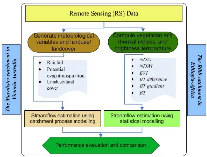
A research design was built around the two approaches (i.e. catchment process modelling and statistical modelling) as mentioned in the previous section to achieve the study objectives. First, the methods and techniques were developed to generate selected meteorological variables such as rainfall and potential evapotranspiration as well as landuse/landcover that have an impact on streamflow using the RS data. These variables were then used in the Soil and Water Assessment Tool (SWAT) (Arnold et al., 1998) to generate the required daily streamflow data. Second, vegetation and thermal indices were calculated using RS data. These indices and brightness temperature were used as input variables to estimate daily streamflow with statistical modelling. These input variables were considered as surrogates for meteorological variables that influence streamflow. The schematic diagram for these two approaches is shown in Figure 1.1. These two approaches were carried out using the following four tasks:
Task 1: All relevant data were collected. These data included relevant RS data, ground measured meteorological data and streamflow data for the study period.
Task 2: Algorithms were built to estimate rainfall, potential evapotranspiration, and classify landuse/landcover from RS data.
Task 3: Estimated rainfall, potential evapotranspiration and landuse/landcover were used as inputs to estimate daily streamflow using the SWAT hydrological model.
Task 4: Relevant vegetation and thermal indices were calculated using RS data.
1-11
modelling. These relationships were then used to estimate daily streamflow data.
A brief description of above mentioned four tasks are as below.
Task 1: RS data, streamflow data as well as the required meteorological data were collected during this task. RS data are available since the 1970s from several satellite programs which are operated by diverse nations. Much of these data are available free of charge. The recently introduced Moderate Resolution Imaging Spectroradiometer (MODIS) data were collected under this task. MODIS bands are characterised by very high signal-to-noise ratio (SNR) with moderate spatial resolution (1 km), which is suitable for use in small and medium scale catchments (Thenkabail et al., 2004).
Streamflow data and meteorological data of the selected study areas were available from the Bureau of Meteorology in Australia (for the Macalister catchment), and the National
1-12
Meteorological Agency and Ministry of Power and Water Resources in Ethiopia (for the Ribb catchment). These data were collected from the above mentioned organizations.
Task 2: High temporal resolution (3 hourly) but low spatial resolution Tropical Rainfall
Measuring Mission (TRMM) data and low temporal resolution (daily) but high spatial resolution MODIS brightness temperate data were used to estimate daily rainfall. Daily potential evapotranspiration data were estimated using RS data by employing the surface energy balance method (Su, 2002; Glenn et al., 2007; Gamage et al., 2011b). Surface emissivity, surface albedo and surface temperature obtained through RS data were used in this process. The performance of these estimates were assessed through Root Mean Square Error (RMSE) and Nash-Sutcliffe efficiency (Ef). The supervised classification approach
with the maximum likelihood classifier was used to classify landuse/landcover for both catchments using reflectance data and vegetation index data. Ground-truth data were used in the supervised image classification process to train the images and hence acquire a higher level of classification accuracy (Gamage et al., 2007).
Task 3: SWAT (Arnold et al., 1998) is a physical-based semi-distributed model that was developed to assess the impact that changing land management practices has on streamflow, nutrients and soil erosion of the catchments. This model can use variables which are estimated from RS data as an input variables. Thus, in this project, variables estimated under Task 2 were used as inputs to the SWAT model of the catchments to estimate daily streamflow. The performance of these estimates were assessed through Root Mean Square Error (RMSE) and Nash-Sutcliffe efficiency (Ef).
1-13
estimate daily streamflow. Artificial neural networks models were developed as statistical models in this study. The performance of the models was assessed through RMSE and Ef.
1.6
Research significance
Continuous streamflow data records are essential for the assessment of water resources and environmental flows, for the quantification of available water for agriculture, and for various other water resources and hydrological analyses. Whilst the use of in-situ stream gauges is the traditional way of collecting these data, such gauging stations are often sparse and declining in numbers, especially in developing countries. It is also appreciated that managing stream gauge networks is laborious and costly, and institutional and political barriers in some countries limit the accessibility of such data to various users. These reasons are the motivation for hydrologists to develop innovative and alternative methodologies to obtain essential streamflow data which have no or less dependency on stream gauge networks.
This project used RS data with minimum ground data as an alternative way of obtaining daily streamflow data for reasonably long records and at less costs. These RS data have the added advantage of better representation of the ground coverage over large areas. Most of the RS data are now freely available and well maintained according to international best practice standards.
1.7
Outline of the thesis
Chapter 2 discusses the past work relevant to the topic. This includes reviews of streamflow modelling using catchment process and statistical modelling approaches, the estimation of meteorological and landuse variables (precipitation, potential evapotranspiration and landuse/landcover) using RS data, and the estimation of vegetation and thermal indices using RS data.
1-14
calculation of vegetation and thermal indices. Finally, the chapter closes with a discussion of the catchment process modelling and statistical modelling approaches used in this thesis.
Chapter 4 presents the application of the methodology (detailed in Chapter 3) to the Macalister catchment. This chapter first discusses the results obtained with regards to the estimation of input variables (rainfall, potential evapotranspiration and landuse/landcover) using RS data. These data were used as inputs to the SWAT model of the catchment and the results of the SWAT model were thereafter compared with ground measured data. The performance of the estimated streamflow is also discussed in this chapter. A similar description is given for statistical modelling in this chapter with respect to input variables and the statistical models. The input variables for statistical modelling were made up of vegetation and thermal indices and brightness temperature. The artificial neural networks was the modelling technique that was used for statistical modelling. Chapter 5, which pertains to the Ribb catchment, follows the same structure as that of Chapter 4.
2-1
2
CHAPTER 2: STREAMFLOW ESTIMATION USING
REMOTE SENSING – A CRITICAL REVIEW
2.1
Introduction
Streamflow in a given catchment is the aggregated result of all geological and climatological factors that operate in that catchment (Herschy, 1995). Knowledge of the availability of streamflow (i.e. both temporal and quantity) forms the basic foundation of any water management project. Therefore, measuring streamflow is important to good water management practices. According to Herschy (1995), Sivapalan (2003) and Sutcliffe (2004), streamflow is the only component of the hydrological cycle that is confined in well-defined channels, as the rest of the components such as rainfall, evapotranspiration and soil moisture are spatially distributed. Therefore the measurement of streamflow provides higher confidence than measurement of other components (Sivapalan, 2003).
The amount of water that flows in well-defined channels (whether a stream or a river) in a given time period defines streamflow data or streamflow record. Streamflow data are important for planning, designing and operating water resource projects that deal with irrigation water supply, hydroelectric power generation, and urban and industrial water supply (Grimes and Diop, 2003). They are also important in monitoring the efficiency and sustainability of such projects. This was highlighted by Sutcliffe (2004) who claimed that streamflow is the most important and directly applicable variable for monitoring and evaluating water resources projects.
2-2
planning, designing and evaluation of water resource projects. This situation is exacerbated due to increased negligence in maintaining the streamflow gauges properly especially since the benefits of such gauging network are invisible and difficult to account for accurately (Herschy, 1995).
The above mentioned issues can be handled to a certain degree by estimating streamflow using meteorological variables. For such purposes, various models can be used and many of these existing models were briefly described by Singh and Woolhiser (2002). For the successful estimation of streamflow, these models require data of meteorological variables, as well as the appropriate values of catchment and model parameters. However, the availability of data of meteorological variables is poor in most parts of the world, especially in developing countries. As a consequence, many studies have attempted to estimate these meteorological variables with RS data. These were briefly described in Chapter 1. Several attempts have also been made to estimate streamflow directly with RS data.
This chapter will review the literature on RS applications aimed at estimating meteorological variables such as rainfall and potential evapotranspiration. In addition, landuse/landcover classification with RS data will also be reviewed. It will further review the applications of RS based meteorological variables in catchment process modelling. Finally, the use of RS data for estimating indices and their use in streamflow estimation with statistical models will be elaborated.
2.2
Streamflow estimation
2-3
The streamflow estimation model was initially introduced to the hydrological world by Mulvarny (1850), as a modelling approach based on a ‘rational’ method. Four decades later, Imbeau (1892) introduced a different dimension to hydrology, presenting an ‘event-based’ model. This model particularly focused on storm peak runoff and rainfall intensity. Subsequently, in the first half of the 20th century, important scientific innovations were developed to understand the hydrological cycle. These innovations were related to physical and biological processes within the catchment, and opened the way to the emergence of many streamflow estimation models. Additionally, this era of hydrological applications was strengthened by Sherman (1932) who introduced the ‘unit hydrograph’ concept. The latter concept was a breakthrough in the calculation of runoff with excess rainfall in a given rain event. Concurrently, Horton (1933) introduced the ‘infiltration theory’ and ‘hydrograph separation’ techniques, while Lowdermilk (1934) and Hursh and Brater (1944) introduced the subsurface water movement component into hydrology. Later, Thornthwaite (1948) and Penman (1948) contributed significantly to hydrology with their understanding and quantification of evapotranspiration, as an abstraction of the hydrological cycle.
2-4
models. These models vary based on their internal processes, and requires a variety of meteorological variables and catchment and model parameters to enable them to estimate streamflow. Given the limited data availability, selecting a particular model for an application can prove to be a challenging task. However, the classification of streamflow estimation models provides guidance on the suitability of models for different context.
2.2.1
Classification of streamflow estimation models
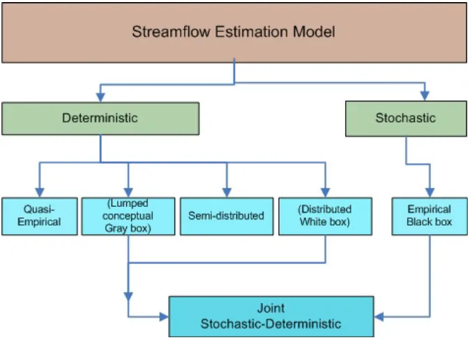
The classification of streamflow estimation models has started as early as 1970s (Woolhiser, 1973; Fleming, 1975). Later, Singh (1995) proposed a classification scheme for the existing streamflow estimation models based on their building process. Based on this idea, all streamflow estimation models were classified into six categories, namely; process description, time scale, space scale, land-use, model use and technique of solution. Since this classification is derived from the model building process, it has only one hierarchical level, with all six categories being equally important. The American Society of Civil Engineers (ASCE) (1996) proposed an alternative classification mechanism for flood analysis models under the headings of (i) event-based rainfall runoff models, (ii) continuous precipitation runoff models, (iii) steady flow routing models, (iv) unsteady flow routing models, (v) reservoir regulation models, and (v) flood frequency models (ASCE, 1996). Since this classification is based on the objective of flood condition simulation (Singh and Woolhiser, 2002), it neglected other existing streamflow estimation models which are used for planning and operating water resources systems.
2-5
2.3
Remote sensing
The emergence of remote sensing (RS) stemmed from the development of conventional, multispectral and infrared photography, non-photographic sensors and scanners, platforms for RS such as aircraft and satellites, launching vehicles, communication and data transmission, data processing and computer technology and other relevant infrastructure (Lillesand and Kiefer, 1999). Importantly, with the advent of RS, the observation regions of the electromagnetic spectrum have expanded far beyond the range of human. This has significant implications for data collection and subsequent predictive analysis.
The term ‘remote sensing’ was initially used by Evelyn L. Pruitt of the USA Office of Naval Research in the early 1960s to denote satellite images which were markedly different from conventional cameras. These images used both visible light and other parts of the electromagnetic spectrum, and as such represented a clear difference from the conventional photography which relies on visible light only. This led to the development of RS as a separate field in the science of data application. Lillesand and Kiefer (1999) defined RS as ‘the technique of obtaining information about an object without physical contact, as opposed to in-situ sensing in which the measuring device is in touch with the
2-6
object’. According to this definition, the emitted or reflected electromagnetic energy of an object is measured by a sensor as part of the RS process. However, this definition was narrowed down by Joseph (2005) following the UN general assembly resolution A/RS/41/65, at the 95th plenary meeting in 1986. According to this later definition, remote sensing is the ‘sensing of the earth’s surface from space by making use of the properties of electromagnetic wave emitted, reflected or diffracted by the sensed objects, for the purpose of improving natural resources management, landuse and the protection of environment’. This second definition successfully captures the aims of RS unlike the broader definition set forward by Lillesand and Kiefer (1999).
2.3.1
History of remote sensing
The history of RS is intricately linked to World Wars I and II. The rapid development of RS technology took place during World War I. After this war, the technology and corresponding experts were adapted and used for civilian applications. (Lillesand and Kiefer, 1999; Joseph, 2005). The launch of Earth Resources Technology Satellite-1 (ERTS 1) by NASA in 1972 which was the parts of work started in the 1960s, was the landmark in the history of RS, and is arguably the beginning of modern RS (Estes, 2005; Irons, 2011) with respect to the civilian applications. This series was later named ‘Landsat’, and was the first of several earth-orbiting satellites designed specifically for land observation for civil applications. The Landsat program provides systematic and repetitive observation of the oceans, atmosphere and land areas (Taylor, 2014). In the recent past, various stakeholders such as the Indian Space Research Organization (ISRO), European Space Agency (ESA), Centre national d'études spatiales – the French space agency (CNES) and Japan Aerospace Exploration Agency (JAXA) have developed numerous sensors with various capabilities and have launched satellites to provide better data for the user community.
2.3.2
The remote sensing system
2-7
passive. Sensors which carry electromagnetic radiation of specific wavelength or band of wavelengths to illuminate the earth’s surface are called active sensors, while sensors that capture natural radiation, which is emitted or reflected from the earth are called passive sensors (Joseph, 2005).
The next step involved in the RS system pertains to the fact that the energy either contained in or impinging on the object of interest is subsequently reflected, absorbed, scattered or emitted. Once this energy leaves the object, it is picked up by the remote sensor (collector). The remote sensor will then transforms the data and finally transmits signals to the receiving center. These remote sensors are embedded with four different resolutions (Joseph, 2005; Lillesand and Kiefer, 1999), namely they are:
• Spatial resolution – the ability of the sensor to separately identify two different objects. Therefore, the higher the spatial resolution, the smaller the object that can be identified.
• Spectral resolution – the spectral bandwidth within which data are collected.
• Temporal resolution (revisit time) – the ability to view the same target under similar conditions at regular intervals.
• Radiometric resolution – the ability to differentiate between two targets based on their reflectance/remittance difference.
The vehicle upon which the remote sensor is mounted is called the platform (i.e. satellite, air plane balloon).
The final step of the RS system is the acquisition of transmitted data by ground station/s. This data are recorded on hardware, and are released to data analysts for processing and interpretation. The level of processing and interpretation of RS data are directly linked with the applications.
2.3.3
Satellites and sensors on board
2-8
MTSAT and KALAPANA are geo-stationary satellites which acquire data on higher temporal resolution. Thus, they are more sensitive to the temporal changes, but have low spatial resolutions. MODIS and AVHRR are sun-synchronized, but have medium spatial and temporal resolution. Spatiotemporal characteristics and the applications of Landsat, MODIS and Tropical Rainfall Measuring Mission (TRMM) satellites are briefly discussed here, since they are important in this study.
Landsat
The Landsat series of satellites have the longest historical records in RS data collection, with these records starting in the early 1970s. The National Aeronautics and Space Administration (NASA) has successfully operated the Landsat series (Landsat 1, 2, 3, 4, 5, 6, 7 and 8) throughout the last 40 years, and has continually improved the sensor features from Landsat 1 to Landsat 8.
A variety of applications is possible with Landsat because of the diversity of sensors with different bands operating on board. The blue band has been used in the applications of water body penetration (Benny and Dawson, 1983; Harrington Jr et al., 1992), coastal water mapping (Gamage and Smakhtin, 2009), soil/vegetation discrimination (Gamage et al., 2009b) and forest feature identification (Oguro et al., 1999; Pax-Lenney et al., 2001). However, the blue band has its own limitations in terms of scattering due to the range of electromagnetic spectrum. Therefore incoming radiance to the sensor is often insufficient in intensity. To address this problem, the green band is used as an alternative for vegetation discrimination and vigor assessment. The red band has been used to measure chlorophyll absorption (Tucker, 1979) of vegetation. The Near Infrared (NIR) band is the most important band among all visible range bands, as it enables the determination of vegetation types, vigor and biomass (Tucker, 1979), and delineates water bodies (Islam et al., 2008). These bands have been prominent in the mapping of landuse/landcover in many studies (Pax-Lenney et al., 2001; Shupe and Marsh, 2004; Jackson et al., 2004; Gamage et al., 2007).
2-9
Sánchez et al., 2008; Oguro et al., 2011). Among all the applications mentioned earlier, those related to landuse/landcover and evapotranspiration can directly be used for streamflow estimation, and are consequently of interest in this study.
Terra and Aqua satellites
The Moderate Resolution Imaging Spectroradiometer (MODIS) is the primary sensor on board of the Terra and Aqua satellites. This sensor is used for monitoring the terrestrial ecosystem in the NASA’s Earth Observing System (EOS) program (Justice et al., 2002). The MODIS sensor is the predecessor of the Advanced Very High Resolution Radiometer (AVHRR). MODIS is very sensitive to the changes in vegetation dynamics (Huete et al., 2002), and was found to be a more accurate and versatile instrument to monitor global vegetation conditions than the AVHRR (Justice et al., 2002). The narrow bands that represent vegetation qualities facilitate this accuracy, and because of this ability, MODIS based vegetation indices give a better representation of landuse/landcover parameters.
2-10
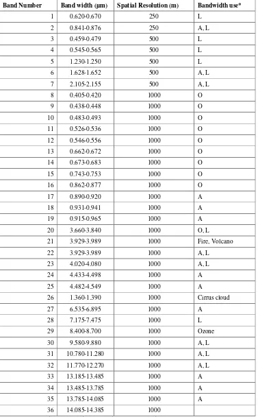
Table 2.1 Band widths and spatial resolution of the MODIS sensor
Band Number Band width (µm) Spatial Resolution (m) Bandwidth use*
1 0.620-0.670 250 L
2 0.841-0.876 250 A, L
3 0.459-0.479 500 L
4 0.545-0.565 500 L
5 1.230-1.250 500 L
6 1.628-1.652 500 A, L
7 2.105-2.155 500 A, L
8 0.405-0.420 1000 O
9 0.438-0.448 1000 O
10 0.483-0.493 1000 O
11 0.526-0.536 1000 O
12 0.546-0.556 1000 O
13 0.662-0.672 1000 O
14 0.673-0.683 1000 O
15 0.743-0.753 1000 O
16 0.862-0.877 1000 O
17 0.890-0.920 1000 A
18 0.931-0.941 1000 A
19 0.915-0.965 1000 A
20 3.660-3.840 1000 O, L
21 3.929-3.989 1000 Fire, Volcano
22 3.929-3.989 1000 A, L
23 4.020-4.080 1000 A, L
24 4.433-4.498 1000 A
25 4.482-4.549 1000 A
26 1.360-1.390 1000 Cirrus cloud
27 6.535-6.895 1000 A
28 7.175-7.475 1000 L
29 8.400-8.700 1000 Ozone
30 9.580-9.880 1000 A, L
31 10.780-11.280 1000 A, L
32 11.770-12.270 1000 A, L
33 13.185-13.485 1000 A
34 13.485-13.785 1000 A
35 13.785-14.085 1000 A
36 14.085-14.385 1000
2-11
The most common applications of MODIS relate to vegetation and seasonal dynamic assessments (Huete et al., 2002; Justice et al., 2002; Thenkabail et al., 2005; Huete et al., 2006; Colditz et al., 2007; de Silveira et al., 2007). MODIS data have also been widely used in evapotranspiration (ET) estimation on various scales from catchment to global level (Kuo et al., 2005; Mu et al., 2007; Guerschman et al., 2009; Zhang et al., 2009b). Such ET information have further been used in water productivity measurements (Gamage et al., 2009b), and have improved rainfall runoff modelling (Zhang et al., 2009b). Furthermore, calculated ET has widely been used in root zone soil moisture assessments (Schnur et al., 2010). More than this, MODIS has been widely used in oceanic, atmospheric and forestry applications.
The Landsat onboard sensors and the MODIS sensor are restricted to the visible, infrared and thermal regions of the electromagnetic spectrum. Therefore, acquiring information related to the internal structure of clouds is difficult, since they are unable to penetrate the cloud cover. This can be avoided by using microwave sensors, which have cloud penetration capabilities. Thus, Tropical Rainfall Measuring Mission (TRMM) Microwave Imager (TMI) and Precipitation Radar (PR) sensors onboard of the TRMM satellite can be used to acquire information of internal structure of clouds.
Tropical Rainfall Measuring Mission satellite
The Tropical Rainfall Measuring Mission satellite is a platform for a collection of sensors to acquire data from many aspects of the atmosphere and clouds in order to estimate precipitation in tropical regions. The group of sensors on board of this satellite includes the Precipitation Radar (PR), TRMM Microwave Imager (TMI), Visible and Infrared Scanner (VIRS), Cloud and Earth Radiant Energy Sensor (CERES) and Lightning Imaging Sensor (LIS) (Kummerow et al., 1988).
2-12
fire circles in tropical regions (Giglio, 2007) and in the retrieval of latent heating profiles of the atmosphere (Shoichi et al., 2009).
2.4
Streamflow estimation using remote sensing data
RS data are used in various forms in different modelling approaches to estimate streamflow. Indeed, both catchment process modelling and statistical modelling approaches have been used with RS data to estimate streamflows in various spatiotemporal scales (Ottlé et al., 1989; Hardy et al., 1989; Giacomelli et al., 1995; Minnas and Hall, 1996; Andersen et al., 2002; Boegh et al., 2004; Chen et al., 2005; Wesseling and Feddes, 2006; Campo et al., 2006; Asante et al., 2008; Stisen et al., 2008; Milzow et al., 2009; Yong et al., 2012).
2.4.1
Use of catchment process models
Catchment process models with various RS based inputs have been used to estimate streamflow in the past (Andersen et al., 2002; Boegh et al., 2004; Campo et al., 2006; McMichael et al., 2006). These inputs estimated from RS data are rainfall (Stisen et al., 2008; Yong et al., 2012), evapotranspiration (Droogers and Kite, 2002; Chen et al., 2005) landuse/landcover (LULC) and Leaf Area Index (LAI) (Andersen et al., 2002; Gamage et al., 2007), and soil moisture (Giacomelli et al., 1995). The application of rainfall, evapotranspiration and LULC to estimate streamflow in catchment process modelling is discussed in the remaining part of this section.
2-13
estimate streamflow, and found a minor improvement in runoff statistics when rainfall estimated from RS data was used as an input in a catchment in West Africa.
Andersen et al. (2002) used the MIKE SHE model (a fully distributed hydrological model) to estimate streamflow in West Africa with estimated rainfall based on GPI. They concluded that the introduction of estimated rainfall, and estimated rainfall complimented with ground measured rainfall did not improve the model’s results. They also concluded that the improvement of rainfall estimates from RS data could improve the accuracy of streamflow estimates.
The introduction of the TRMM satellite took place in late 90’s and the sensors onboard this satellite are dedicated to measuring rainfall from space. The data of these sensors not only cover the majority of the globe but they also give more information on clouds and hence to improve the accuracy of rainfall estimation compared to previous rainfall estimates that were based on visible and thermal infrared data. Especially, TRMM microwave sensor data empowered existing rainfall estimation procedures by adding structural information on clouds (Huffman et al., 1995; Huffman et al., 2007). Since then, TRMM data have been used to produce various precipitation products such as 3B42 (Huffman et al., 2007), and have been extensively applied in hydrology.
2-14
Collischonn et al. (2008) used ground measured and TRMM 3B42 rainfall data to simulate streamflow separately in a very large catchment (>460,000 km2). They compared the simulation results of both models with observed streamflow data, and concluded that the performance of the model based on TRMM 3B42 rainfall data is as good as that with the model with ground measured data at the most downstream gauge point of the catchment. In the same study, they tested several upstream gauge points in which case they found that the performance of estimated streamflow with TRMM 3B42 rainfall data was reduced towards the upstream of the catchment, i.e. with decreasing catchment area. Nikolopoulos et al. (2010) used TRMM 3B42, KIDD (a rainfall product that was estimated on the algorithm proposed by Kidd et al. (2003)), radar and ground measured rainfall data in streamflow estimation to investigate the relationship between the error of satellite based rainfall data and the size of the catchment. In this study, they concluded that the error in streamflow estimation increased while catchment size decreased. They highlighted that the use of rainfall products of higher spatial resolution could alleviate the error propagation in small catchments. In sum, above studies showed that the spatial representation of TRMM rainfall data is not sufficient enough to estimate streamflow accurately in medium and small size catchments.
2-15
Landuse/landcover classified using RS has also been widely used in streamflow estimation. These landuse/landcover maps have been extensively used in defining crops area, and the hydrological model has mainly been used to define the cropping pattern and the rest of the parameters (Boegh et al., 2004). The LULC information computed from RS data has been used as early as 1977 (Pluhowski, 1977) to improve estimates of streamflow characteristics. It was concluded that landuse/landcover information of RS provides an effective means of significantly improving estimates of streamflow. Even though landuse/landcover has widely been used in streamflow estimation as an input, landuse/landcover has been considered as a time constant variable in most of the applications.
Landuse/landcover has not only been used as input to streamflow estimation, but it has also been utilized to investigate the impact on hydrology due to LULC changes (Githui et al., 2009; Dadhwal et al., 2010; Gumindoga, 2010). Gumindoga (2010) used RS data to classify landuse/landcover over the Gilgal Abay catchment in Blue Nile in Ethiopia, and thereafter used it in the TOPMODEL hydrological model to investigate the impact of landuse/landcover changes on the hydrology of the catchment. Gumindoga (2010) concluded that RS data not only helped to achieve the objectives of the study, but also facilitated the derivation of vital information for planning and implementation of development projects, especially in ground measured data scarce areas like Ethiopia. Moreover, Vaze et al. (2011) used landuse/landcover information obtained from RS data to estimate regional model parameters of Sacramento and SIMHYD models. They then used these parameters to estimate streamflows in ungauged catchments in Australia.