Croton, Darren (2005): Galaxy Formation and Evolution: The Local Galaxy Population as a Cosmological Probe. Dissertation, LMU München: Fakultät für Physik

(1)

Galaxy Formation and Evolution:

the Local Galaxy Population as a

Cosmological Probe

Dissertation der Fakultät für Physik

der

Ludwig-Maximilians-Universität München

vorgelegt von Darren J. Croton

aus Melbourne, Australia

Datum der mündlichen Prüfung: 3. November 2005

(2)

(3)

Summary

We take a multi-faceted approach to study galaxy populations in the local universe, us-ing the completed Two Degree Field Galaxy Redshift Survey (2dFGRS), the “Millennium Run”ΛCDM N-body simulation, and a semi-analytic model of galaxy formation. Our in-vestigation covers both small and large scale aspects of the galaxy distribution. This work can be broken into three sections, outlined below.

Using the 2dFGRS we explore the higher-order clustering properties of local galaxies to quantify both (i) the linear and non-linear bias of the distribution relative to the under-lying matter field, and (ii) the nature of hierarchical scaling in the clustering moments of the galaxy distribution. This last point is the expected signature of an initially Gaussian distribution of matter density fluctuations that evolved under the action of gravitational instability. We show in Chapters 2, 3, and 4 that the 2dFGRS higher-order clustering mo-ments are indeed hierarchical, which we measure up to sixth order for galaxies brighter than MbJ −5 log10h = −17 and which sample the survey volume out to z ≈ 0.3. The moments are found to be well described by the negative binomial probability distribution function, and we rule out, at high significance, other models of galaxy clustering, such as the lognormal distribution. This result holds in redshift space on all scales where we obtain a good statistical signal, typically 0.5 < R (h−1Mpc) < 30 (i.e. from strongly non-linear to quasi-linear regimes). Interestingly, we find that the moments on larger scales can be significantly altered by two massive superclusters present in the 2dFGRS. The skewness of the galaxy distribution is found to have a weak dependence on galaxy luminosity. We show that a simple linear biasing model provides an inadequate description of the higher order results, suggesting that non-linear biasing is present in the clustering moments of the 2dFGRS.

(8)

(9)

1 Introduction

1.1 Motivation

Much of my work as a PhD student has centred on an attempt to understand two important aspects of the nature of galaxies in the local universe. The first considers a larger scale perspective of the galaxy population: (i) How are galaxies distributed across the billions of light years that we currently observe? (ii) How do these galaxies reflect the underlying dark matter density field? (iii) What does this tell us about the initial conditions of the universe, before all the structure that we currently see came into being? On the other hand, the second aspect of interest can be considered, by comparison, a rather small scale perspective of the galaxy population: (i) Can we explain the rich diversity of individual galaxies and galaxy associations seen in the local universe? (ii) Are there key aspects to our understanding of galaxy formation and evolution that we are missing? (iii) How important is the environment around a galaxy in determining its final properties, the so called nature or nurture question. This thesis represents a culmination from the past three years of my work on these problems. Perhaps not surprisingly, with such a broad range of questions to be investigated, this research remains ongoing and includes numerous collaborations, both locally and internationally. Extensions beyond this thesis are discussed in the final chapter. Any study of the large scale structure of the galaxy distribution and the evolution of galaxy populations inside this distribution must begin with an understanding of the inter-play between matter and gravity. Below I provide a brief overview of basic cosmology theory and the equations which govern it. The evidence for dark matter is presented along with its place in the larger scheme of structure formation. I give a short introduction to galaxy clustering and bias, followed by a discussion of the Two Degree Field Galaxy Redshift Survey and a basic overview of the state of current models of galaxy formation. Finally, I finish with a outline of the scientific objectives of each chapter in this thesis.

1.2 Essential cosmology

(10)

The strongest force by far in the universe on large scales is gravity, and any study of large scale behaviour must begin with an understanding of it. To formalise the mathematical theory of gravity, one is required to introduce the concept of a space-time interval between two events, ds, and look for stationary values of Rds, which correspond to the shortest

distance between any two points being a straight line. This space-time interval defines the metric, and in general relativity it describes the space-time geometry in which particles naturally move.

The most general space-time metric describing a universe in which the cosmological principal is obeyed is the Robertson-Walker metric (Coles & Lucchin 1995):

ds2 =c2dt2₋a(t)2 _dr2

1₋kr2 +r

2_(d_θ2₊_sin2_θ_d_φ2₎_, _(1.1)

where we have used standard spherical polar coordinates r,θ,φ(all co-moving), t is the proper-time, a(t) is the cosmic scale factor, and the constant k is the curvature parameter, which can be scaled to only take on the values -1, 0 or 1. This metric defines a metric tensor,gi j, with which the Robertson-Walker metric takes the form:

ds2=g_{i j}dxidxj, (1.2)

where the Einstein summation convention is implied.

Having the Robertson-Walker metric tensor allows us to use general relativity to obtain equations for the time evolution of the scale factor a(t). The basic Einstein field equations of general relativity are differential equations which relate the geometry of space-time (the metric) to the distribution of energy and momentum within it (the source terms for gravity). These equations can be written as:

Ri j− 1

2Rgi j =− 8πG

c2 Ti j−Λgi j , (1.3)

where Ti j is the total energy-momentum tensor, Ri j is the Ricci tensor (a function of the metricg_{i j}), R=Rii is a measure if the curvature of space-time, andΛis Einstein’s famous cosmological constant, which has become very important in recent years. If the Robertson-Walker metric tensor is substituted into the Einstein field equations, along with Ti j =

diag(ρ,₋p,₋p,₋p) assuming the simplest case of a perfect fluid, one obtains the following

equations for the time evolution of the scale factor a:

¨a

a =−

4πG

3

ρ+ 3p c2

+ Λ

3 , (1.4)

˙a a

2

= 8πG

3 ρ+

Λ

3 −

k

a2 . (1.5)

(11)

1.3 The “dark” universe

density parameter) where ρ_crit = 3H2/8πG (the critical density), the second Friedmann

equation can be recast as:

k

H2_a2 = Ωtot−1. (1.6)

In this form, it is easy to see that, since H2a2is always greater than zero, there is a corre-spondence between the sign of the curvature parameter k and the sign ofΩtot−1. If k equals 1, the density of the universe must exceed the critical density, and its ultimate fate is for gravity to win and for it to collapse back in on itself. On the other hand, if k equals ₋1, the density must be less than critical, and then the expansion must win. The case of k= 0 corresponds to an equilibrium between gravity and expansion, implying that the geometry of the universe is flat.

In this way, we see that the energy density of the universe describes its underlying ge-ometry, which in turn has a direct effect on its ultimate fate: expand forever in a big freeze or collapse back in on itself in a big crunch. The cosmological constant, Λ, adds an ex-tra element that decelerates or accelerates the expansion, depending on its sign. Current observations suggest that the universe is flat. We will discuss this and the effects of the cosmological constant shortly.

1.3 The “dark” universe

Given the importance of Ω_tot in understanding the global nature and ultimate fate of the universe, it is only natural that its accurate measurement is high on the priority list of astronomers. Numerous methods have been developed to do this, and their conclusions were as interesting as they were profound. We summarise a few of these below, and refer the reader to Longair (1998) and Peebles (1980) for a more detailed account.

Possibly the simplest way to determineΩtot comes from calculating the mean mass den-sity of galaxies in the universe,ρ_gal:

ρ_gal = _L_ρ_gal _M

L

, (1.7)

where_Lρgal is the mean luminosity density of galaxies, and<M/L>is the mean galaxy

mass-to-light ratio. A value of _Lρgal is obtainable from the galaxy luminosity function,

while < M/L> can be determined directly from the rotation curves of spiral galaxies. FromΩgal = ρgal/ρcrit, the result follows. Putting these measurements together, one finds thatΩgal ≈ 0.01−0.03 for varying galaxy samples, which is a very low result if we have any reason to expect a critical density universe.

A second method to determineΩ_totutilises observations of galaxy clusters. To measure the mass of a galaxy cluster, one firstly requires the velocity dispersion_hσ2_iof the galaxies within the cluster. If we assume that the cluster is gravitationally bound, then the mass of the cluster follows from the cosmic virial theorem:

2KE+PE = 3

2

σ2 Mvir−

GMvir

Rvir

(12)

An estimate ofρ_vir, and hence Ω_vir, can thus be obtained by simply summing the masses of a number of large clusters within some set distance. By this technique, the value of the density parameter is found to beΩvir ≈0.1−0.3, an order of magnitude higher thanΩgal, but still 3 to 10 times smaller than what is required for a flat universe.

Adding up the luminous matter in galaxies and balancing the energy equation for clus-ters are not the only indicators of a discrepancy in our accounting of the mass content of the universe. Strong evidence came in the late 1970’s when the rotation curves of spiral galaxies were accurately measured (e.g. Freeman 1970) for the first time. Interestingly, it was found that at large radii from the galactic centre the rotational velocity seemed to flatten, and by the measurement of gas surrounding the galaxy at radio wavelengths, this rotational flattening extendeds to greater radii than the visible mass of the galaxy. This is in contrast to the simplified expected Keplerian behaviour of the visible component, for which the velocity decreases as the inverse square root of the radius. Such rotation curve measurements indicate that virtually all spiral galaxies have a dark, diffuse halo associated with them that contributes at least 3 to 10 times the mass of the visible matter (Kormendy 1982). This conclusion is in line with that found by measuring the mass content of clusters. Two interesting conclusions follow from these results. First, it indicates that there is a large dark component dominating cluster and galaxy masses. Understanding the nature of this “dark matter” has spawned a whole new subfield of cosmology. Second, by the fact that we’re still a long way short ofΩ_tot _≈ 1, either the above measurements suggest that much more mass is hidden somewhere else in the universe away from groups and clusters, up to 10 times more, or it hints at the existence of a cosmological constant which acts such that the sum ofΩ_m+ ΩΛ≈1. There is much theoretical motivation (e.g. inflation), as well as detailed CMB observations (Spergel et al. 2003) and supernovae distance measurements (Riess et al. 1998), which all indicate that the universe is very nearly flat. This suggests that some form of “dark energy,” in addition to the dark matter, is required in order to fit the measured properties of the observable universe.

The theory for cold dark matter was worked out in response to these problems, and more generally to understand structure formation in the universe. The standard model for cold dark matter (CDM) typically includes: a cosmological component of dark matter with negligible thermal velocity, a scale free power spectrum of initial adiabatic density fluctuations, and a dark energy or cosmological constant component, chosen so as to make

(13)

1.4 Large scale structure, galaxy clustering and bias

Given the above standard model of cosmology, one can investigate the effects of gravita-tional instability and the evolution of large scale structure in the universe. This is achieved by tracing the time evolution of the initial matter density perturbation field, δI(x). Un-der the influence of its own gravity, an initial Gaussian density field will evolve into a strongly non-Gaussian one, resulting in a rich diversity of form that is characteristic of a highly evolved distribution of matter. In the favoured ΛCDM scenario discussed above, the formation of structure is expected to proceed hierarchically from the initial density perturbations, with galaxies forming first and larger structures following later from the merging of galaxies. The most striking feature revealed in all large-scale galaxy redshift surveys has been the way that galaxies are typically distributed along sheets and filaments, with empty voids between them. These structures have been seen to be as large as 50 to 100 Mpc. Understanding how such structures came to be is one of the primary goals of modern cosmology.

The observed structure in the universe can be characterised by the clustering moments of the distribution of density fluctuations,δ(x). Here we model the spatial distribution of galaxies as realizations of statistically homogeneous and isotropic random point processes. The 2-point correlation function, or second moment of the distribution, ξ2(R), is defined by the conditional probability of finding a galaxy in the volume element dV at a distance

R from a galaxy, beyond that expected for a Poisson distribution (Peebles 1993):

dP=N [1¯ +ξ₂(R)] dV, (1.9)

where ¯N is the mean density of galaxies. The 2-point correlation function can also be

understood as the Fourier transform of the power spectrum, P(k) = _h|δ(k)_|2_i. Note that the 2-point function is a complete description of the field only in the case of a Gaussian distribution. For more realistic cases, one requires the higher order p-point moments, ξp(R). We explore the higher order correlation function of the observed galaxy distribution in detail in Chapters 2, 3, and 4.

Interestingly, it was quickly realised that galaxies had to be a biased tracer of the under-lying density field. This can be seen by comparing the 2-point galaxy-galaxy correlation function and cluster-cluster correlation function. Such observations reveal that, although both correlation functions have the same power law slope, the cluster-cluster correlation function has an amplitude approximately 20 times larger. If both galaxies and clusters arise from the same gravitational instability and amplification of the initial density field, then this observation indicates that distinct samples of galaxies must trace the underlying mass distribution in different ways. This phenomenon is generally known as galaxy bias.

(14)

the most massive clusters can correspond to _∼ 4σ fluctuations, explaining the very low spatial density of such rare objects. Density fluctuations of lower amplitude, such as those which represent isolated galaxies, will collapse on longer timescales and be distributed in a way that is more representative of the overall mass distribution.

In the simplest picture, bias is usually quantified as the relative clustering strength of galaxies with respect to the underlying dark matter through the 2-point correlation func-tion:

ξ₂gal =b2ξDM₂ , (1.10)

where b is the ubiquitous linear biasing term. As always, the true picture is not quite this simple, however. Both linear and non-linear bias are possible in the galaxy distribution, and this is an effect we will explore using both the low and higher order clustering moments of the observed galaxy distribution.

1.5 Observed and mock galaxy populations

In this thesis we will exploit both observed and simulated galaxy catalogues. Both are of such quality that we can undertake statistical analyses of unprecedented accuracy. We now give a brief description of both.

The Two Degree Field Galaxy Redshift Survey

The Two Degree Field Galaxy Redshift Survey (2dFGRS) is an international collaboration which has had the ambitious aim of measuring the redshifts of approximately 250,000 galaxies in the local universe (Colless et al. 2001, 2003). This has been made possible with the use of the 2dF multi-fibre spectrograph on the Anglo-Australian Telescope, which is capable of observing 400 objects simultaneously over a 2 degree field. The catalogue is sourced from a revisited and extended version of the APM galaxy catalogue (Maddox et al. 1990), and the targets are galaxies with extinction corrected magnitudes brighter than bJ=19.45.

The main survey area covers approximately 2000 deg2 and has a median depth of z =

0.11. The area is centred on two declination strips, one in the southern galactic hemi-sphere spanning 80◦×15◦ close to the south galactic pole, and the other in the northern galactic hemisphere spanning 75◦_×10◦ along the celestial equator (Fig. 1.1). In this the-sis, catalogues will be built with galaxies from both regions. At the effective limit of the survey, z _≈0.3, the strips contain an approximate volume of 108h−1Mpc3(forΩ_m = 0.3,

ΩΛ = 0.7). An additional 99 random fields are distributed around the southern galactic cap but are not used in this work.

(15)

1.5 Observed and mock galaxy populations

Figure 1.1: An all sky plot of the APM/2dFGRS survey area. The individual 2dFGRS fields are marked as small circles, with the larger south galactic pole region lying to the right of the figure, and the smaller more north galactic pole region on the left.

parameter Q in the range of 1-5, with 5 being of highest quality and 1 being the poorest. An accurate statistical analysis of the final galaxy catalogue required spatial and magni-tude incompleteness to be compensated for. This was achieved in the standard way by defining three masks through which the data was processed: (1) a magnitude limit mask giving an extinction corrected apparent magnitude limit as a function of position on the sky, (2) a redshift completeness mask providing the fraction of measured redshifts at each position, and (3) a magnitude completeness mask linking redshift success rate with appar-ent magnitude. These masks also include holes, which define the excluded regions from the survey area due to effects such as foreground stars and plate flaws, for example. The overall average redshift completeness of the parent catalogue is found to be 91.8%.

(16)

un-wanted objects and badly sampled galaxies. To do this, we choose only galaxies with apparent magnitudes in the range 14.0 < m < mlim, where mlim varies as a function of angle on the sky (<mlim> = 19.37), redshifts within the range 0.002 < z < 0.5, to avoid selecting stray stars or quasars, and a redshift quality of at least Q_≥3, to ensure accurate distance estimation. From the 221,414 unique redshifts obtained, the above constraints provide 194,407 quality redshifts with which to do our analysis – 113,895 in from the SGP region and 80,512 from the NGP region. This galaxy catalogue forms the basis with which we undertake our analyses in Chapters 2, 3, 4 and 5.

Galaxy formation models

To understand many problems in astronomy, including those specific to galaxy formation and the galaxy population as a whole, astronomers have often turned to the exploration of potential solutions through computer simulations. In this field, two important and com-plimentary techniques have developed over the last 10 or so years. Hydrodynamic simu-lations follow the co-evolution of both gas and dark matter explicitly, and this approach has been integral to understanding many astrophysical phenomena. However, due to the heavy computational cost of hydrodynamic methods, they are usually limited in either size or resolution when compared with pure N-body techniques. To circumvent these short-comings one can instead take a ‘semi-analytic’ approach (e.g. White & Frenk 1991) based on the galaxy formation paradiam outlined by White & Rees (1978). In the semi-analytic picture, the physics important to galaxy formation is modelled analytically in parallel to the numerical evolution of pure N-body dark matter. Its power lies in the relatively minor computational cost of implementation, and this allows for speedy exploration of parameter space around many different models relating to the question at hand. We will follow this second approach.

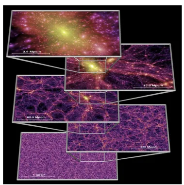
The galaxy formation model we use in Chapter 6 is implemented on top of a very large dark matter simulation of the concordanceΛCDM cosmology. We have dubbed this sim-ulation the ‘Millennium Run’ because of its size and resolution (Springel et al. 2005 – see Fig. 1.2). The Millennium Run follows the dynamical evolution of 21603 _'₁_.₀₀₇₈_×₁₀10 dark matter particles in a periodic box of 500 h−3Mpc3, which implies a mass resolution per particle of 8.6_×108h−1M. We adopt cosmological parameter values consistent with a combined analysis of the 2dFGRS (Colless et al. 2001) and first year WMAP data (Spergel et al. 2003; Seljak et al. 2004). They areΩm = Ωdm+ Ωb =0.25,Ωb =0.045, h =0.73,

ΩΛ=0.75, n=1, andσ8=0.9.

Friends-of-friends (FOF) halos are identified in the simulation using a linking length of 0.2 the mean particle separation, while sub-structure within each FOF halo is found with an improved and extended version of the SUBFINDalgorithm of Springel et al. (2001). Having determined all halos and subhalos at all output snapshots, we then build the hier-archical merging trees that describe in detail how structures grow as the universe evolves. These trees form the backbone onto which we couple our model of galaxy formation.

(17)

1.5 Observed and mock galaxy populations

Figure 1.2: The Millennium RunΛCDM N-body simulation. Each panel represents a magnification by factors of four, highlighting the rich structure the simu-lation can resolve. The colour coding is by local density and dark matter velocity dispersion.

(18)

1.6 Thesis overview

This thesis is a collection of five papers, four of which are published in the Monthly No-tices of the Royal Astronomical Society (MNRAS, Chapters 2–5), and the last of which has recently been submitted to the MNRAS. In this body of work we cover three main areas of research: (i) the higher order clustering of the large scale distribution of the lo-cal galaxy population (Chapters 2–4), (ii) the environmental dependence of the luminosity function for early and late type galaxy populations (Chapter 5), and (iii) the way in which the suppression of cooling flows shape the properties of the massive galaxy population (Chapter 6). We now give a brief overview of each of these chapters in turn.

Higher order clustering in the local universe

The first half of this thesis, Chapters 2, 3, and 4, describe a study of the higher-order clustering in the 2dFGRS. In Chapter 2 we measure the clustering moments of the local

L_∗ galaxy population using a volume limited sample contained a total of 44,931 galaxies within the magnitude range ₋19 > MbJ − 5 log10h > −20 and survey volume defined

by 0.02 < z < 0.13. Using this probe, we investigate if the p-point galaxy correlation functions, ¯ξp, can be written in terms of the two point correlation function or variance, ¯

ξ_p=Spξ¯₂p−1, for some constant hierarchical scaling values, Sp. This is the so-called hi-erarchical scaling hypothesis, and is expected if an initially Gaussian distribution of den-sity fluctuations evolves under the action of gravitational instability. The quality of our measurement is such that we can measure the moments up to sixth order across scales 0.3 < R (h−1Mpc) < 30. We compare our results with those from the Hubble Volume

ΛCDM N-body simulation to look for signatures of non-linear biasing between the galax-ies and underlying dark matter halo density field. In this chapter, we also discuss the impact of two rare, massive superclusters in the 2dFGRS volume on the higher order clustering moments of the L_∗galaxy distribution.

In Chapter 3 we take this analysis one step further by measuring the higher order mo-ments of the 2dFGRS galaxy distribution as a function of galaxy luminosity. We use the full survey, approximately 200,000 galaxies, and build volume limited catalogues in one magnitude bins covering the magnitude range₋17> MbJ −5 log10h>−22, sampling the

spatial distribution of galaxies out to scales of z≈0.3 (∼ 750h−1Mpc). With these galaxy samples, we investigate how hierarchical scaling in the clustering distribution varies with galaxy luminosity, again up to sixth order. Past analyses have shown that the hierarchical scaling coefficients, Sp = ξ¯p/ξ¯₂p−1, are approximately independent of scale, and we look for this behaviour as well. As in Chapter 2, the influence of two massive superclusters in the 2dFGRS is quantified, especially on large scales where their presence is most likely to be seen. Chapter 3 also provides a comprehensive analysis of both linear and non-linear biasing in the galaxy distribution. We investigate the relative bias in the 2dFGRS, with respect to the L_∗ population, as a function of luminosity using the clustering moments. The results of this chapter generalise those found in Chapter 2.

(19)

“re-1.6 Thesis overview

verse” approach to the previous method by measuring the reduced void probability function (VPF) of the galaxy distribution in volume limited catalogues covering magnitudes from

MbJ −5 log10h=−18 to−22. The VPF connects the distribution of voids to the moments of galaxy clustering of all orders. The reduced VPF can be used to both measure hierar-chical scaling in the clustering moments and to discriminate between different clustering models that make predictions for how this scaling should arise. Such models include the lognormal distribution and the negative binomial model, which we show we can discrimi-nate between at a high significance. Thus, the predictive power of the reduced VPF makes this chapter a valuable extension to the previous two. In addition, as the reduced VPF is weighted more by the lower and intermediate counts in the galaxy probability distribution function, we show that these results are insensitive to superclusters in the 2dFGRS volume, unlike the results of the previous two chapters. We also measure the reduced VPF for dark matter in aΛCDM universe and compare to that found for the galaxy population.

Environmental dependence of the galaxy luminosity function

In Chapter 5, we shift our focus from the spatial distribution of the local galaxy population to the properties of galaxies that lie within this distribution. Here we study the luminosity functions of galaxies in different large-scale density environments, from sparse voids to the densest cluster regions. To do this, we develop a new method to measure the environmental dependent luminosity function and demonstrate that it gives comparable results to previ-ous methods but with the added bonus of simultaneprevi-ously providing the luminosity function normalisation as well as shape. Our analysis includes the separation of the galaxy popu-lation into early and late spectral types. Using the Schechter function parameterisation of the luminosity function, we measure the characteristic luminosity and faint-end slope in each environment. This parametrisation allows us to demonstrate the smooth change in the galaxy population between extremes in density and, when examined as a function of spectral type, quantifies the differences between the galaxies in clusters, mean density, and void regions of the universe, for both early and late types. We finish with a discussion of our results in light of current galaxy formation models.

Cooling flows and the properties of massive galaxies

(20)

(21)

2 Hierarchical galaxy clustering in the

2dFGRS

1 Abstract

We use the two-degree field Galaxy Redshift Survey (2dFGRS) to test the hierarchical scaling hypothesis: namely, that the p-point galaxy correlation functions can be written in terms of the two point correlation function or variance. This scaling is expected if an initially Gaussian distribution of density fluctuations evolves under the action of gravita-tional instability. We measure the volume averaged p-point correlation functions using a counts-in-cells technique applied to a volume limited sample of 44,931 L_∗ galaxies. We demonstrate that L_∗ galaxies display hierarchical clustering up to order p = 6 in red-shift space. The variance measured for L_∗ galaxies is in excellent agreement with the predictions from a Λ-cold dark matter N-body simulation. This applies to all cell radii considered, 0.3 < (R/h−1Mpc) < 30. However, the higher order correlation functions of

L_∗galaxies have a significantly smaller amplitude than is predicted for the dark matter for

R < 10h−1Mpc. This disagreement implies that a non-linear bias exists between the dark matter and L_∗galaxies on these scales. We also show that the presence of two rare, mas-sive superclusters in the 2dFGRS has an impact on the higher-order clustering moments measured on large scales.

2.1 Introduction

Current theoretical models of structure formation in the Universe are based on the paradigm of gravitational instability. This process is believed to be responsible for driving the growth of small primordial density perturbations into the nonlinear collapsed structures such as galaxies and clusters that are evident in the Universe today.

The premise of gravitational instability has been tested indirectly by comparing the clus-tering predicted by numerical simulations of the formation of cosmic structures with the observed distribution of galaxies (e.g. Benson et al. 2001). A direct test of this fundamen-tal ingredient of structure formation models was made using the 2dFGRS by Peacock et al. (2001). The size of the 2dFGRS allowed the first accurate measurement of the two-point

1_{C.M. Baugh, D.J. Croton, E. Gaztañaga, P. Norberg, M. Colless, et al. (the 2dFGRS Team), MNRAS, 351,}

(22)

galaxy correlation function on large scales. Peacock et al. demonstrated that the two-point correlation function at large pair separations displays a form that is characteristic of the bulk motions of galaxies expected in the gravitational instability scenario.

We present an independent test of the gravitational instability paradigm. For a Gaus-sian distribution of density fluctuations, the volume averaged correlation functions, ¯ξ_p, are identically zero for p>2; the density field is completely described by its variance, ¯ξ2. The evolution of an initially Gaussian density field due to gravitational instability generates non-zero ¯ξ_p(Peebles 1980). A basic test of the gravitational origin of the higher order mo-ments is to determine their relation to the variance of the distribution. This is traditionally encapsulated in the hierarchical model:

¯

ξ_p=Spξ¯₂p−1. (2.1)

This model applies to real space clustering; however, in redshift space the scaling still tends to hold even on small scales where the “fingers-of-God” effect is prominent (Lahav et al. 1993; Hoyle, Szapudi & Baugh 2000). Perturbation theory predicts that the hier-archical amplitudes for the mass distribution are independent of the cosmological density parameter, the cosmological constant and cosmic epoch (Bernardeau et al. 2002).

We use the 2dFGRS (Colless et al. 2001, 2003) to measure the higher order correlation functions of the galaxy distribution, focusing on the clustering of L_∗galaxies. The size of the 2dFGRS is exploited to extract a volume limited sample of L_∗galaxies, which greatly simplifies our analysis (Section 2.2). The results for the volume averaged correlation func-tions, up to sixth order, are presented in Section 2.3, in which we also test how well the hierarchical scaling model works. Our conclusions are given in Section 2.4.

2.2 Data and analysis

The density of galaxies is a strong function of radial distance in a magnitude limited sur-vey. This needs to be compensated for in any clustering analysis by applying a suitable weighting scheme (e.g. Saunders et al. 1991). Alternatively, one may construct a volume limited sample by selecting certain galaxies from the full redshift survey. These galaxies are chosen so that they would appear inside the apparent magnitude range of the survey if displaced to any redshift within the interval defining the sample. The only radial vari-ation in galaxy number density in a volume limited sample is due to large scale structure in the galaxy distribution. This makes volume limited samples much more straightforward to analyse than flux limited samples. However, only a fraction of the galaxies from the full redshift survey satisfy the selection criteria in redshift and absolute magnitude. This reduction in the density of galaxies has curtailed the utility of volume limited subsamples constructed from earlier redshift surveys.

(23)

2.2 Data and analysis

Figure 2.1: The projected galaxy density in the L_∗ volume limited sample, smoothed on two different scales. The galaxy distribution is projected onto the right ascension–redshift plane and is then smoothed in circular cells of radius 15h−1_{Mpc (left) and 3h}−1_{Mpc radius (right). Redder colours denote higher}

densities as indicated by the key that accompanies each panel. Two “hot-spots” stand out clearly, particularly in the left hand coneplots; one in the NGP at z _≈0.08 and the other in the SGP at z _≈0.11. Right ascension is given in radians.

larger redshifts and thus sample larger volumes. However, brighter than L_∗, the space density of galaxies drops exponentially (e.g. Norberg et al. 2002b). Hence, the optimum balance between volume surveyed and intrinsic galaxy space density is achieved for L_∗ galaxies. In addition, the higher order clustering of L_∗ galaxies provides a benchmark or reference against which to compare trends in clustering strength with galaxy luminosity (see Norberg et al 2001; Croton et al. 2004b). We consider the two contiguous areas of the 2dFGRS, referred to as the NGP and SGP regions, which contain around 190,000 galaxies with redshifts and cover an effective area of approximately 1200 square degrees in total. After selecting galaxies with absolute magnitudes in the range₋19> MbJ−5 log10h>−20 (corrected to z =0 using the global k+e correction quoted by Norberg et al. 2002b), the

(24)

z = 0.021 to 0.130, corresponding to a volume of 7.97_×106h−3Mpc3for the combined NGP and SGP regions.

2.2.1 Counts-in-cells

The distribution of counts-in-cells is estimated by throwing down a large number of spher-ical cells, on the order of 107for each cell radius considered, within the L_∗volume limited 2dFGRS sample. Full details of how we deal with the spectroscopic incompleteness and the angular mask are given in Croton et al. (2004b); the corrections turn out to be small in any case (see figure 1 of Croton et al.).

The higher order correlation functions, ¯ξp, are the reduced pth order moments of the distribution of galaxy counts-in-cells. The estimation of the higher order correlation func-tions from the cell count probability distribution is explained in a number of papers (e.g. Gaztañaga 1994; Baugh, Gaztañaga & Efstathiou 1995; Croton et al. 2004b). The variance or width of the count distribution is given by the case p = 2. For p > 2, the correlation functions probe further out into the tail of the count probability distribution.

We use mock 2dFGRS catalogues to estimate the errors on the measured higher order correlation functions. Full details of the mocks can be found in Norberg et al. (2002b) and Croton et al. (2004b).

2.3 Results

The projected density of galaxies in the L_∗volume limited sample is shown in Fig. 2.1. The galaxy density projected onto the right ascension–redshift plane is smoothed using circu-lar windows. Two different smoothing radii have been used to produce these maps; the left-hand panel shows the density after smoothing with a circular cell of radius 15h−1_Mpc and the right hand panel shows the distribution as sampled with a cell of radius 3h−1Mpc. The redder colours indicate higher galaxy densities, as shown by the scale that accom-panies each cone plot. Two ‘hot-spots’ are readily apparent, particularly in the cone plot smoothed on the larger scale. These correspond to superclusters of galaxies that also ap-pear in the 2dFGRS Percolation Inferred Galaxy Group catalogue (Eke et al. 2004) and in the reconstructed density field of the 2dFGRS (Erdogdu et al. 2004). The presence of these superclusters has an impact on the extreme event tail of the count probability distri-bution. Later in this section, we will investigate the influence of these structures on our measurement of the higher order correlation functions by excising the volumes that con-tain the superclusters from our analysis. The ‘cosmic web’ of filamentary structures and voids is apparent in the cone smoothed on the smaller scale.

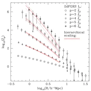
The higher order correlation functions measured for L_∗ galaxies are plotted in Fig. 2.2. The correlation functions are only plotted on scales for which a robust measurement is possible. The correlation functions show a dramatic steepening on small scales as the or-der p increases. For example, the ratio ¯ξ₆/ξ¯₂is 105 at R = 1h−1Mpc, falling to_∼ 100 at

(25)

dis-2.3 Results

Figure 2.2: The higher order correlation functions ¯ξp measured for L∗ galaxies in the 2dFGRS (symbols). The orders p = 2–6 are shown, as indicated by the key. The errorbars show the rms scatter estimated using mock 2dFGRS cata-logues. The lines show the ¯ξpmeasured for the dark matter in redshift space

in theΛCDM Hubble Volume simulation, for orders p=2 to 6 in sequence of increasing amplitude for R<10h−1Mpc.

tribution in theΛCDM Hubble Volume simulation (Evrard et al. 2002). These theoretical predictions include the effects of peculiar motions in the distant observer approximation. The variance of the dark matter in redshift space agrees spectacularly well with the mea-sured ¯ξ₂ for L_∗ galaxies. This confirms the conclusions reached in independent analyses of the clustering of L_∗ galaxies in the 2dFGRS (Lahav et al. 2002; Verde et al. 2002). However, for the case of theΛCDM Hubble Volume simulation, the p>2 moments of the dark matter differ from the measurements for L_∗galaxies for R<10h−1Mpc.

(26)

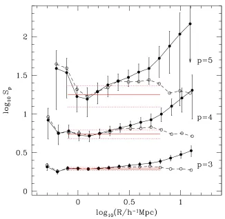
Figure 2.3: The hierarchical amplitudes, Sp, for p=3,4 and 5, plotted as a function of

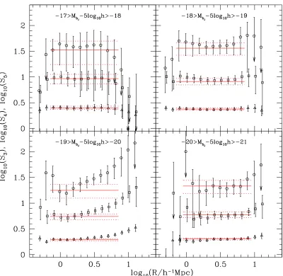
cell radius for the L_∗volume limited sample. The filled symbols connected by solid lines show the results obtained using the full volume. The best fit constant values of Spare shown by the horizontal solid lines, which are

plotted over the range of scales used in the fit. The dotted lines show the 1₋σerror on the fit. The open symbols connected by dashed lines show the hierarchical amplitudes recovered when the two largest superclusters are masked out of the volume.

(27)

2.3 Results

Figure 2.4: The higher order correlation functions, ¯ξp, measured for L∗galaxies in the 2dFGRS (symbols, as in Fig. 2) compared with the predictions of the hierar-chical model (Eq. 2.1; solid lines). The hierarhierar-chical predictions are plotted only on the scales used to fit Sp. The dotted lines indicate the errors on these

predictions, with contributions from the error on the fitted value of Sp and

on the measured variance ¯ξ2.

2002). We therefore attempt to fit a constant value of Sp to the ratios plotted in Fig. 2.3. We use a principal component analysis to take into account the correlation between the

¯

ξpin neighbouring bins (e.g. Porciani & Givalisco 2002; for further details of our imple-mentation see Croton et al. 2004b). The results of this analysis are given in Table 2.1. In Fig. 2.3, the horizontal lines show the best fit constant value for Sp, fitted over the scales 0.71 < (R/h−1Mpc) < 7.1. The same range of scales is used to fit the Sp for each order

(28)

order Sp ±2σ χ2/ndof 3 1.95 0.18 6.1 4 5.50 1.43 2.8 5 17.8 10.5 1.9 6 46.3 50 1.1

Table 2.1: The best fit values for Sp and the 2−σerror (∆χ2 = 4), obtained using the

measurements for cell radii in the range 0.71_≤(R/h−1Mpc)_≤7.1. The 2₋σ errors are approximately twice the size of the 1−σerrors. The final column gives the reducedχ2 using the number of degrees of freedom derived from the principal component analysis.

Sp are extremely correlated, with the principal component analysis showing that the first few eigenvectors contain the bulk of the variance, indicating that there are typically just 2 or 3 independent points. Sample variance leads to measurements which could be coher-ently shifted either low or high with respect to a fixed value. This therefore drives the best fit value of Sp to lie either below or above a sizeable fraction of the data points. For the

L_∗sample, we note that neither S3nor S4are particularly well described by a constant fit (see the reducedχ2values in Table 2.1).

For purely illustrative purposes, we have carried out the experiment of removing the two superclusters from the L_∗ volume limited sample and repeating our measurement of the higher order correlation functions. The corresponding results for the hierarchical ampli-tudes are plotted using open symbols in Fig. 2.3. The upturn in the Spvalues at large radii is no longer apparent. Rather than being considered as a correction, the results of this ex-ercise simply serve to show the influence of the supercluster regions on our measurements of the ¯ξ_p. Where the difference matters, it effectively indicates that the volume of even the 2dFGRS is too small to yield a robust higher-order clustering measurement. A further discussion of this test is given by Croton et al. (2004b).

(29)

2.4 Conclusions

We have measured the higher order correlation functions of L_∗galaxies up to sixth order in the 2dFGRS. Previous studies of galaxy clustering in redshift space have been lim-ited to fourth order (e.g. for optically selected samples: Gaztañaga 1992; Benoist et al. 1999; Hoyle et al. 2000: for infra-red selected samples: Bouchet et al. 1993; Szapudi et al. 2000). The volume limited sample of L_∗ galaxies analysed here contains 100 times more galaxies and covers 10 times the volume of the previous best measurements from an optically selected galaxy redshift survey (Hoyle et al. 2000). The measured correla-tion funccorrela-tions have a form that is in remarkably good agreement with the prediccorrela-tions of hierarchical scaling, and extend to smaller scales than those for which the perturbation theory predictions are expected to be valid (Bernardeau et al. 2002). A similar conclusion was reached by Croton et al. (2004a), who found hierarchical scaling in the reduced void probability function measured in the 2dFGRS.

On scales larger than about 4h−1Mpc, there is an upturn in the values of Sp, which we have demonstrated is influenced by the presence of two large superclusters in the 2dFGRS (see Fig. 2.3). This suggests that finite sampling affects our measurements on these scales. A similar feature was found in the angular Edinburgh-Durham Southern Galaxy Cata-logue (EDSGC). Szapudi & Gaztañaga (1998) found that the projected Spmeasured from the EDSGC displayed an up-turn for scales larger than 0.5 degrees, which corresponds to ≈ 4h−1Mpc at the characteristic depth of the survey. The EDSGC covers a similar part of the sky to the 2dFGRS. This feature in Sp was not found, however, in the APM Survey, which covers a four times larger solid angle than the EDSGC (Gaztañaga 1994). This behaviour is not seen in the mock catalogues drawn from theΛCDM Hubble Volume sim-ulation. Intriguingly, an upturn in the hierarchical amplitudes on large scales is expected in structure formation models with non-Gaussian initial density fields (Gaztañaga & Fosalba 1998; Bernardeau et al. 2002).

Finally, we note that the variance of the distribution of cell counts for L_∗ galaxies is in excellent agreement with the predictions for CDM, obtained from the Hubble Volume

ΛCDM simulation, which includes the effects of peculiar motions on the clustering pattern. However, for cells with radii R < 10h−1Mpc the higher order correlation functions of L_∗ galaxies have significantly lower amplitudes than the dark matter. This implies that the relation between the distribution of galaxies and the underlying dark matter may be more complicated than the popular linear bias model, suggesting that nonlinear contributions to the bias may be important on small and intermediate scales (Fry & Gaztañaga 1993; see also the analyses by Conway et al. 2005 and Wild et al. 2005). We note that on large scales (R > 10h−1Mpc), the ¯ξp measured for L∗ galaxies agree better with the ΛCDM

predictions, supporting the conclusion reached previously, that on these scales, L_∗galaxies approximately trace the mass distribution (Gaztañaga & Frieman 1994; Lahav et al. 2002; Verde et al. 2002).

(30)

(31)

3 Higher order clustering in the 2dFGRS

1 Abstract

We measure moments of the galaxy count probability distribution function in the two-degree field galaxy redshift survey (2dFGRS). The survey is divided into volume limited subsamples in order to examine the dependence of the higher order clustering on galaxy luminosity. We demonstrate the hierarchical scaling of the averaged p-point galaxy cor-relation functions, ¯ξ_p, up to p = 6. The hierarchical amplitudes, Sp=ξ¯p/ξ¯₂p−1, are ap-proximately independent of the cell radius used to smooth the galaxy distribution on small to medium scales. On larger scales we find the higher order moments can be strongly affected by the presence of rare, massive superstructures in the galaxy distribution. The skewness S3has a weak dependence on luminosity, approximated by a linear dependence on log luminosity. We discuss the implications of our results for simple models of linear and non-linear bias that relate the galaxy distribution to the underlying mass.

3.1 Introduction

The pattern of galaxy clustering can be quantified by measuring the galaxy count proba-bility distribution function (CPDF) on a range of smoothing scales. The CPDF gives the probability that a randomly chosen region of the universe will contain a particular num-ber of galaxies, and is typically expressed as a function of both the size of the region smoothed over and the galaxy number within that volume. Traditionally, most effort has been directed at measuring the second moment of the count distribution, the variance,

¯

ξ2, through the autocorrelation function or, equivalently, its Fourier transform, the power spectrum (e.g. Percival et al. 2001; Padilla & Baugh 2003; Tegmark et al. 2004). The higher order moments of the CPDF, expressed as volume averaged correlation functions,

¯

ξp (p=2,3, . . .), provide a much more detailed description of galaxy clustering, probing the shape of the low and high count tails of the distribution.

The higher order moments of the dark matter distribution are known to display a hier-archical scaling in which the p-point volume averaged correlation functions, ¯ξp, can be written in terms of the variance of the count distribution, ¯ξ₂: ¯ξ_p = Spξ¯₂p−1 (e.g. see Pee-bles 1980, Juszkiewicz, Bouchet & Colombi 1993, Bernardeau 1994, Baugh, Gaztañaga

1_{D.J. Croton, E. Gaztañaga, C.M. Baugh, P. Norberg, M. Colless, et al. (the 2dFGRS Team), MNRAS, 352,}

(32)

& Efstathiou 1995, Gaztañaga & Baugh 1995, Fosalba & Gaztañaga 1998). This scal-ing is a signature of the evolution under gravitational instability of an initially Gaussian distribution of density fluctuations. A remarkable feature of the scaling is that the values of the hierarchical amplitudes, Sp, on scales for which the density field evolves linearly or in a quasi-linear fashion, are insensitive to cosmic epoch and essentially independent of the cosmological density parameter or the value of the cosmological constant. For a comprehensive review of such results see Bernardeau et al. (2002) and references therein. Departures from the hierarchical scaling of the higher order moments could conceivably arise in three ways:

(i) A strongly non-Gaussian distribution of primordial density waves as could arise, for instance, due to a seed non-linear fluctuation such as a global texture (see Gaztañaga & Mahonen 1996, Gaztañaga & Fosalba 1998, Scoccimarro, Sefusatti & Zaldarriaga 2004 for examples of how the Sp scale in this case). This avenue now seems un-likely, following the clear detection of multiple acoustic peaks in the power spectrum of cosmic microwave background temperature fluctuations (Netterfield et al. 2002; Hinshaw et al. 2003; Mason et al. 2003; Scott et al. 2003; Kuo et al. 2004); such peaks are difficult to reconcile with models that include cosmological defects (Kamionkowski & Kowsowsky 1999). Moreover strongly non-Gaussian primordial fluctuations are ruled out by the first year WMAP results (Komatsu et al. 2003; Gaztañaga & Wagg 2003)

(ii) A weakly Gaussian distributed primordial density field, resulting from a non-linear perturbation to a Gaussian density field. This scenario is difficult to distin-guish from the evolution of an initially Gaussian field under gravitational instability, because the perturbation can introduce a shift to the amplitudes Spthat is also hierar-chical. This can happen even in the case where the non-linear perturbation produces a negligible effect on the power spectrum (Bernardeau et al. 2002).

(iii) The spatial bias between the galaxy distribution and the underlying distribution of dark matter. Fry & Gaztañaga (1993) demonstrated that, under a local biasing pre-scription, the hierarchical scaling of the higher order moments is preserved but the amplitudes Sp can change as a function of time or luminosity. This conclusion is also reached using more sophisticated, physically motivated semi-analytic models of galaxy formation (Kauffmann et al. 1999; Benson et al. 2000; Scoccimarro et al. 2001).

(33)

3.1 Introduction

& Gaztañaga 1994, Ghigna et al. 1996, Feldman et al. 2001). Such analyses were typ-ically limited to measuring the three and four point correlation functions. The nature of the dependence of the hierarchical amplitudes on luminosity has not been convincingly established. Recent work to investigate this in the optical (Hoyle et al. 2000) and in the far infrared (Szapudi et al. 2000) was restricted to probing fairly narrow ranges of luminosity due to the size of the redshift surveys then available.

The advent of multi-fibre spectrographs exploited by sustained observing campaigns has led to a new generation of redshift survey which represents order of magnitude advances over surveys completed in the last millennium. The Sloan Digital Sky Survey (York et al. 2000) and the Two-degree Field Galaxy Redshift Survey (2dFGRS, Colless et al. 2001) have provided maps of the clustering pattern of galaxies with unprecedented detail. Anal-ysis of the 2dFGRS clustering has suggested that the flux limited sample could be an essentially unbiased tracer of the dark matter in the Universe (Lahav et al. 2002; Verde et al. 2002) 2. These results confirmed previous deductions about galaxy bias (e.g. Gaz-tañaga 1994, Frieman & GazGaz-tañaga 1999, GazGaz-tañaga & Juszkiewicz 2001) reached using the parent angular catalogue of the 2dFGRS, the APM Galaxy Survey (Maddox et al. 1990, 1996). The 2dFGRS covers a volume that is an appreciable fraction of that sampled by the APM Survey, with full redshift coverage (modulo the relatively small redshift incomplete-ness that still remains). This means that for the first time, a measurement of the higher order moments is possible in three dimensions with comparable accuracy to that attain-able in two dimensions, but without the added complication of the effects of projection (Gaztañaga & Bernardeau 1998; Szapudi & Gaztañaga 1998).

The sheer number of galaxies in the 2dFGRS allows it to be subdivided in order to probe the dependence of the clustering signal on intrinsic galaxy properties in more detail. Norberg et al. (2001) found that the amplitude of the projected two point correlation function scales with luminosity, and characterised this trend using a relative bias factor with a linear dependence on luminosity. In this paper we extend the work of Norberg et al. to study the higher order clustering of galaxies in the 2dFGRS and its dependence on luminosity. Our approach is the same as that followed in Baugh et al. (2004), who measured the higher order correlation functions of a sample of L_∗galaxies and found that they follow a hierarchical scaling.

We provide a brief review of the measurement of the moments of the CPDF in Section 3.2. In Section 3.3, we discuss the specific application of this method to the 2dFGRS; an important feature of our analysis is the use of mock catalogues to estimate the errors on our measurements (see Section 3.3.3). Our results for the higher order correlation functions and the hierarchical amplitudes are given in Section 3.4. We quantify the variation of the higher order moments with luminosity in Section 3.5, and discuss the interpretation of these results in terms of a simple relative bias model. Our conclusions are set out in Section 3.6. Throughout, we adopt standard present day values of the cosmological parameters to compute comoving distance from redshift: a density parameter Ωm = 0.3

2_{Note that with the weighting scheme adopted to compensate for the radial selection function, the}

(34)

and a cosmological constantΩΛ=0.7.

3.2 Counts-in-cells statistics

The count probability distribution function (CPDF) and its moments have been used ex-tensively to quantify the clustering pattern of galaxies (e.g. White 1979; Peebles 1980). In this Section we give an outline of the counts-in-cells approach, explaining how the volume averaged p-point correlations are derived from the CPDF and give a brief theoretical back-ground. A more comprehensive discussion of the counts-in-cells approach can be found in Bernardeau et al. (2002).

3.2.1 Estimating thep-point volume averaged correlation functions

The p-point moment, or (un-reduced) correlation function, m3(r1,r2,r3)≡< δ(r1)...δ(rp)>, can be used to fully characterise the clustering of a fluctuating field δ(r). The reduced

p-point correlation function,ξp(r1, ...,rp), is defined as the connected part of the above p-point correlation in such a way that for p>2:ξ_p=0 for a Gaussian field (see Bernardeau et al. 2002 for more details). Following the standard convention, for the remainder of this paper when we talk about correlations we will always assume they are “reduced" correla-tions.

The p-point volume averaged galaxy correlation function, ¯ξ_p(V), can be written as the integral of the p-point correlation function, ξp, over the sampling volume, V (Peebles 1980):

¯

ξ_p(V)= 1 Vp

Z

V

d3r1 . . . d3rpξp(r1, . . . ,rp). (3.1)

A practical way in which to estimate ¯ξp(V) is to randomly throw cells down within the galaxy distribution, recording the number of times a cell contains N galaxies so as to build up the galaxy CPDF, PN(V). Since we adopt spherical cells, the CPDF is a function of the sphere radius, R,

PN(R)= NN NT

, (3.2)

where NN is the number of cells that contain N galaxies out of a total number of cells thrown down, NT. The volume averaged correlation functions ¯ξp(V) are then related to the moments of the CPDF, mp:

mp(R)=h(N−N)¯pi=

∞ X

N=0

PN(R)(N−N)¯p, (3.3)

where ¯N is the mean number of galaxies in a cell of volume V and is calculated directly

from the CPDF

¯

N = ∞ X

N=0

(35)

3.2.2 Scaling of the higher order moments

For the case of a continuous distribution, ¯ξ_pis related to the corresponding cumulant,µ_p, through ¯Npξ¯p=µp, where the cumulants are defined as (see Gaztañaga 1994 for details):

µ2=m2 ; µ3=m3,

µ₄=m4−3m22 ; µ5=m5−10m3m2. (3.5) If instead we are dealing with a discrete distribution, these relations must be corrected. A Poisson shot noise model is adopted (see Baugh et al. 1995 for a discussion of this point), to give corrected estimates of the moments, kp:

k2=µ2−N ;¯ k3 =µ3−3k2−N¯,

k4=µ4−7k2−6k3−N¯,

k5=µ5−15k2−25k3−10k4−N¯. (3.6)

The volume-averaged correlation functions, calculated from the galaxy CPDF, follow di-rectly from the relation ¯ξp=kp/N¯p.

3.2.2 Scaling of the higher order moments

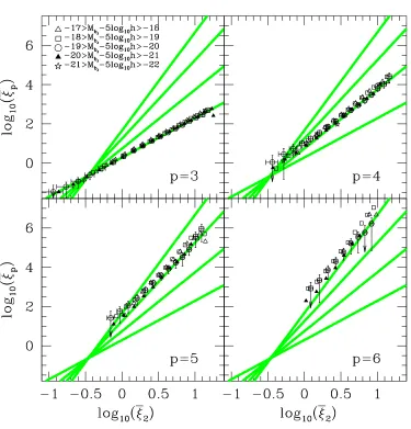
In the hierarchical model of clustering, all higher-order correlations can be expressed in terms of the 2-point function, ¯ξ2, and dimensionless scaling coefficients, Sp:

¯

ξp=Spξ¯₂p−1. (3.7)

Traditionally, S3 = ξ¯3/ξ¯2₂is referred to as the skewness of the distribution and S4 = ξ¯4/ξ¯3₂ as the kurtosis. The hierarchical scaling of the higher order moments arises from the evolution due to gravitational instability of an initially Gaussian distribution of density fluctuations (see Bernardeau et al. 2002 and references therein).

3.2.3 Systematic effects: biased estimators

In addition to sampling errors (see Section 3.3.3 below), the estimation of the hierarchi-cal amplitudes can be compromised by systematic effects, as discussed in some detail by Hui & Gaztañaga (1999). These authors identified two sources of error that could lead to a systematic bias in the inferred values of Sp. The first effect arises from biases in the estimates of the higher order correlation functions themselves, known as the “integral constraint bias” (see e.g. Bernstein 1994). The second effect originates in the nonlinear combination of ¯ξpand ¯ξ2to form Sp; this is called the “ratio bias”. The latter effect dom-inates on large scales and tends to cause the inferred values of the Sp to be biased low. Hui & Gaztañaga wrote down expressions for these biases which accurately reproduce the systematic effects seen upon estimating the hierarchical amplitudes from sub-volumes extracted from N-body simulations.

(36)

is made brighter, the volume of the sample increases. Thus the estimation biases tend to cause the Spto increase with sample luminosity. This spurious tendency has already been reported in the literature (see Hui & Gaztañaga 1999). For volumes of the size used in our analysis, it turns out that the predicted biases are smaller than the corresponding sampling errors (e.g. see figure 3 in Hui & Gaztañaga 1999). This is the first time that a redshift survey has been available which is large enough to overcome such systematic biases.

3.2.4 Galaxy biasing

Galaxy samples constructed using different selection criteria display different clustering patterns. This leads one to the conclusion that distinct samples of galaxies must trace the underlying mass distribution in different ways, a phenomenon that is generally known as galaxy bias.

A simple, heuristic scheme describing the impact of a local bias on the scaling of the higher order moments was proposed by Fry & Gaztañaga (1993). These authors demon-strated that in this case, the scaling of the higher order moments of the galaxy distribution should mirror that of the dark matter, though possibly with different values for the hierar-chical amplitudes Sp. Fry & Gaztañaga made the assumption that the density contrast in the galaxy distribution, δG, i.e. the fractional fluctuation around the mean density, could be written as a Taylor expansion of the density contrast of the dark matter,δDM:

δG= ∞ X

k=0

bk

k!(δ

DM₎k_. _(3.8)

On scales where the variance, ¯ξDM₂ , is small, the leading order contribution to the two-point volume averaged correlation function of galaxies has the form:

¯

ξ₂G=b2₁ξ¯DM₂ , (3.9)

where b1 is the ubiquitous linear bias b. The leading order forms for the hierarchical amplitudes, Sp, for the cases p=3 and p=4 are:

S₃G = 1 b1

SDM₃ +3c2

(3.10)

S₄G = 1 b2₁

SDM₄ +12c2SDM3 +4c3+12c22

, (3.11)

where we use the notation ck = bk/b1. Expressions for the hierarchical amplitudes are given up to p=7 in Fry & Gaztañaga (1993).

(37)

3.2.4 Galaxy biasing

(k=1 and 2) are given by:

b1=1+ ν2₋1

δ_c (3.12)

b2=2 1− 17 21

!

ν2₋1 δc

+ν

2

δ2_c(ν 2

−3) (3.13)

whereν_≡δc/σ(M),δcis the linear theory overdensity at the time of collapse (δc =1.686 forΩ = 1) andσ(M) is the linear rms fluctuation on the mass scale of the halos. This is a simple model but nevertheless it shows some tendencies that are correct. For example, a typical mass halo corresponding to ν= 1 displays an unbiased variance with b1 = 1, but introduces a bias in the skewness, since c2=b2=−0.7. As a further illustration, consider massive halos defined by ν2 > 3; in this case the Mo, Jing & White theory predicts that

c2 > 0, while less massive halos could produce c2 < 0. To get more realistic values of

bk for galaxy bias, a prescription has to be adopted for populating dark matter halos of a given mass with galaxies of a given luminosity (Benson et al. 2001; Scoccimarro et al. 2001; Berlind et al. 2003).

In the interpretation of the higher order moments presented in this paper we will make use of a relative bias, which describes the change in clustering compared with that mea-sured for a reference sample (Norberg et al. 2001, 2002a). Using Eq. 3.9 as a guide, we define the relative bias, br=b1/b∗₁, of a sample as the square root of the ratio of the 2-point correlation function measured for the sample over that measured for the reference sample, denoted by an asterisk (the reference sample will be defined explicitly in Section 3.5):

br≡

b1

b∗₁ = ξ¯G₂

¯ ξG₂∗

1/2

. (3.14)

Thus, we can obtain an estimate of the relative bias from the ratio of the variances. When the linear bias is a good approximation (ck ' 0 for k > 1), we can relate SGp in different galaxy samples regardless of the underlying DM value of Sp:

SG_p = S

G∗

p

bpr−2

. (3.15)

More generally, one can manipulate Eq. 3.10 to write down an expression comparing SG_p for two galaxy samples, eliminating SDM₃ for the underlying dark matter (e.g. see Eq. 9 in Fry & Gaztañaga 1993). For the skewness:

SG₃∗=brSG₃ −3

(c2−c∗₂)

b∗₁ , (3.16)

where an asterisk denotes a quantity describing the reference sample, and br = b1/b∗₁ is the relative bias defined above. Any second order relative bias effects are thus given by:

c0₂= (c2−c ∗ 2)

b∗₁ =

1 3

brSG₃ −SG₃∗