Self-calibration method without joint iteration for distributed small satellite SAR systems

R E S E A R C H

Open Access

Self-calibration method without joint iteration for

distributed small satellite SAR systems

Qing Xu

, Guisheng Liao, Aifei Liu and Juan Zhang

Abstract

The performance of distributed small satellite synthetic aperture radar systems degrades significantly due to the unavoidable array errors, including gain, phase, and position errors, in real operating scenarios. In the conventional method proposed in (IEEE T Aero. Elec. Sys. 42:436–451, 2006), the spectrum components within one Doppler bin are considered as calibration sources. However, it is found in this article that the gain error estimation and the position error estimation in the conventional method can interact with each other. The conventional method may converge to suboptimal solutions in large position errors since it requires the joint iteration between gain-phase error estimation and position error estimation. In addition, it is also found that phase errors can be estimated well regardless of position errors when the zero Doppler bin is chosen. In this article, we propose a method obtained by modifying the conventional one, based on these two observations. In this modified method, gain errors are firstly estimated and compensated, which eliminates the interaction between gain error estimation and position error estimation. Then, by using the zero Doppler bin data, the phase error estimation can be performed well independent of position errors. Finally, position errors are estimated based on the Taylor-series expansion. Meanwhile, the joint iteration between gain-phase error estimation and position error estimation is not required. Therefore, the problem of suboptimal convergence, which occurs in the conventional method, can be avoided with low computational method. The modified method has merits of faster convergence and lower estimation error compared to the conventional one. Theoretical analysis and computer simulation results verified the effectiveness of the modified method.

Keywords:Array signal processing, Distributed small satellite synthetic aperture radar (DSS-SAR) systems, Error estimation

1. Introduction

With the development of spaceborne synthetic aperture radar (SAR) systems, the functions, such as SAR image, ground moving target indication (GMTI), and SAR inter-ferometry (InSAR), have been well performed [1-4]. In the conventional spaceborne SAR systems, large antennas are required due to the minimum antenna area constraint [5]. However, it leads to the failure for the systems to obtain an image of wide area since the illumination area is in-versely related to the aperture size of the antennas [6]. Distributed small satellite synthetic aperture radar (DSS-SAR) systems [6-12] were developed to deal with the problem and have received considerable attention in re-cent years. In DSS-SAR systems, several small satellites

move in a special orbital configuration and function as a single “virtual satellite”. A small antenna covering wide area is placed on each satellite with the total antenna area constituted by all the small antennas satisfying the mini-mum antenna area requirement. Due to the flying forma-tion of DSS-SAR systems, along-track baselines and across-track baselines may exist synchronously. And the across-track baseline is needed for terrain height estima-tion [7] while the along-track baseline is suitable for the function of SAR and GMTI [8]. In [9], the SAR train con-figuration is analyzed and many scholars focus their attention on SAR imaging or GMTI based on this config-uration [10,11]. However, for the echo received by each small satellite, range or azimuth (Doppler) ambiguities will occur due to the use of small antennas. In order to image a wide swath unambiguously, the echoes of small antennas should be combined coherently in the DSS-SAR system.

* Correspondence:[email protected]

National Laboratory of Radar Signal Processing, Xidian University, Xi’an 710071, China

In [10,11], the low pulse repetition frequency (PRF) is chosen to avoid range ambiguity which results in Doppler ambiguity, and the approaches are also given to suppress Doppler ambiguity. However, their excellent performance is critically dependent on the knowledge of the array manifold (parameterized by many parameters, such as angle of arrivals, and antennas’position information). The array manifold is used in coherent combination of small antennas’echoes to suppress Doppler ambiguity [10]. In practice, there always exist various perturbations in the array manifold which are always called as array errors, such as gain, phase, and position errors. Since the array manifold cannot be exactly obtained because of the exist-ence of array errors, the performance of Doppler ambigu-ity suppression [11,12] can significantly be degraded. Therefore, it is necessary to estimate and calibrate array errors prior to carry out Doppler ambiguity suppression. In [12], the array error calibration method has also been discussed.In array error estimation of DSS-SAR systems, the existing array calibration methods [13-18] can be ap-plied to the systems only when proper calibration sources are chosen. In [12], spectrum components within one Doppler bin are used as calibration sources with known directions which are called “virtual calibration sources.” Since the number of spectrum components is more than one due to Doppler ambiguity, it is possible to apply array calibration methods with more than one calibration source [15-18] to DSS-SAR systems. In [12], a two-step it-erative auto-calibration method is presented to estimate gain-phase and position errors. In the first step, assuming that position errors are known, gain-phase errors are estimated by using the method in [16]. In the second step, based on the gain-phase error estimated in the former step, position errors can be obtained by the least squared method [17]. These two steps should be iterated alterna-tively to obtain final solutions. For convenience, the array error estimation method in [12] is named as the conven-tional method (the comparison in this article is limited in terms of array error estimation method).

In the conventional method, two kinds of errors, the gain-phase error and the position error, are respectively estimated under the assumption that other kinds of errors are known. The inherent relationship among gain, phase, and position errors is not considered and analyzed in the conventional method. In this article, by studying of the conventional method, the following two aspects are observed. First, gain error estimation and position error estimation can affect each other, which will influence the convergence rate. And the conven-tional method may even suffer from suboptimal conver-gence in large position errors. Second, if spectrum components within the zero Doppler bin are used as calibration sources to estimate the errors, phase error estimation can be performed independent of position

errors. Based on the above two aspects, a modified array error estimation method is proposed in this article. First, in order to eliminate the interaction between the gain and position error estimations, gain errors are first estimated and compensated. Then, phase errors are estimated by using the spectrum components within the zero Doppler bin as calibration sources. Finally, position errors are estimated based on Taylor-series expansion. However, since Taylor-series expansion causes approxi-mation errors, position error estiapproxi-mation should be iterated in order to obtain higher estimation accuracy. In comparison with the conventional method, the modified method can avoid the iteration between gain-phase error estimation and position error estimation, which guaran-tees that it can converge to optimal solutions with lower computational load and fast convergence speed. Simula-tion results verify that the modified method performs better than the conventional one.

The remainder of the article is arranged as follows. In Section 2, the modified method for DSS-SAR systems is described in detail. The performance of the modified method is verified by using Monte Carlo simulations in Section 3. The article ends with some conclusions given in Section 4.

2. Modified method for DSS-SAR systems 2.1. Signal model

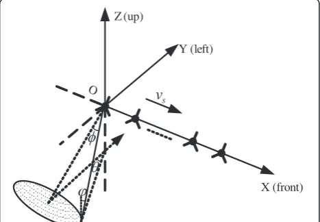
In this article, the signal model of DSS-SAR systems will be introduced briefly as follows [12]. The SAR train con-figuration in which all the satellites are arranged along the X-axis as an array is given in Figure 1. The (X,Y,Z) direction is referred to as (along-track, cross-track, and radial). The array operates in the side-looking strip mode and all satellites have an identical along-track velocity, denoted byvs.θ,φ, andϕrepresent azimuth angle, inci-dence angle, and cone angle, respectively. Azimuth angle θ(τ, fd) can be expressed asθ(τ,fd) =θo+Δθ(τ,fd), where

O

Z (up)

Y (left)

X (front)

s

v

θo and Δθ(τ, fd) are the azimuth angle and the offset from the beam center, respectively. τ denotes the fast time corresponding to the range bin and fd denotes the Doppler frequency which corresponds to the slow time.

True coordinates, measured coordinates, and corresponding position errors of themth satellite are denoted by (xm,ym,

zm), (xmo,ymo,zmo), and (Δxm,Δym,Δzm), respectively. The relationship among them is

xm;ym;zmÞ ¼ðxmo;ymo;zmoÞ þðΔxm;Δym;ΔzmÞ;

ð ð1Þ

where ymo= 0, zmo= 0. The first satellite is taken as reference, i.e., (Δx1,Δy1,Δz1) = (0, 0, 0) is imposed. Then

the clutter echo in the range-Doppler domain received by themth satellite after demodulation in the strip mode and broadside geometry can be written as [12]

Smðτ;fdÞ ¼gmejξm XI

i¼I ej4π

λdmðτ;fdþifrÞ_H

mðτ;fdþifrÞ þnmðτ;fdÞ;

ð2Þ

where gm andξ1are the gain and phase error of themth

array element relative to the first array element (as such,

g1= 1 andξ1= 0).λdenotes the wavelength of the carrier. nm(τ,fd) is the additive white Gaussian noise. 2I+ 1 is the number of spectrum components within one range-Doppler bin. The spectrum components have different azimuth anglesθ(τ,fd+ifr) and the same incidence angles φ(τ) which can be expressed as follows:

fdþifr¼ 2vs

λ sinθ τð ;fdþifrÞsinφð Þτ ; i¼ I;. . .;I: ð3Þ In the following, for simplicity, (•)iis used to denote the variable associated with (fd+ifr), such asθi denotes θ(τ, fd+ifr). dmi =xm sinθi sinφ(τ) +ym cosθi sinφ(τ) +zm cosϕ(τ). In the side-looking strip mode, θo= 0 and then θi

=Δθi. Moreover,Δθi is very small (|Δθi|≤0.43° for a small antenna with the azimuth length of 2 m atX-band) in practice. Thus, cosθi_{= cosΔθ}i_≈

1 can be obtained with small angle approximation. Sinceymo=zmo= 0,

di

m¼ðxmoþΔxmÞsinθisinφð Þ þτ ðymoþΔymÞcosθisinφð Þτ

þðzmoþΔzmÞcosφð Þτ ≈ðxmoþΔxmÞsinθisinφð Þτ

þΔymsinφð Þ þτ Δzmcosφð Þτ

ð4Þ

Hm(τ, fd) is the complex envelope of the clutter echo in the range-Doppler domain,

Hmðτ;fdÞ ¼∬σðx;yÞh τ2rmðx;y;z;fdÞ c

G fð ÞdejΨ 0_x;y;z;f

d ð Þ

dxdy

ð5Þ

where σ(x, y) is the complex surface scattering

coeffi-cient. Ψ0ðx;y;z;fdÞ ¼4π_λ

ffiffiffiffiffiffiffiffiffiffiffiffiffiffi y2þ_z2

p

πλpffiffiffiffiffiffiffiffiffiy2_þz2

2vs2 þ2πfd x vs. h

(τ) is a linear frequency modulated signal.G(fd) denotes the Fourier transform of the function which represents the antenna pattern and other time-variant characters (identical to all receiving antennas). rm(x,y, z, fd) is the slant range from themth satellite to the ground cell,

rmðx;y;z;fdÞ ¼

ffiffiffiffiffiffiffiffiffiffiffiffiffiffi y2þ_z2

p

þλ2

ffiffiffiffiffiffiffiffiffiffiffiffiffiffi y2þ_z2

p

f_d2

8v2 s

Δymcosθ τð ;fdÞsinφð Þτ Δzmcosφð Þτ :

ð6Þ

Since Δymcosθ(τ, fd)sinφ(τ) and Δzmcosφ(τ) can be

neglected inrm(x,y,z,fd), it can be obtained that r1(x,y, z,fd)≈ ⋯ ≈rM(x,y,z,fd)≜r(x,y,z,fd). So, asH1(τ,fd)≈

⋯ ≈HM(τ,fd)≜H(τ,fd).

Based on the previous analysis, (2) can be rewritten as

Smðτ;fdÞ ¼gmejξ 0

mX I

i¼I

ej4λπd0mi_Hiþ_n

mðτ;fdÞ ð7Þ

where

ξ0

m¼ξmþ 4π

λ ðΔymsinϕ τð Þ þΔzmcosφð ÞτÞ; d0mi¼ðxmoþΔxmÞsinθisinφð Þ ¼τ λ

2vs

fdþifr

ð ÞðxmoþΔxmÞ:

It is found that the contributions of position errors to array outputs can be separated into two parts. One part associated with cross-track and radial position errors is fixed for all clutter echoes and can be regarded as array phase errors. The other part related to along-track pos-ition errors changes with spectrum components. For simplicity, the total phase error ξ0m is called the phase error and the along-track position error is named as the position error in the following. The unknown errors considered here are the position errorΔxm(m= 2,. . .,M) and the gain-phase error gmejξ

0

m _{(m= 2,}. . ._{,M). Using} vector notation, Equation (7) can be rewritten as follows

S¼ΓAHþn ð8Þ

where S= [S1,. . ., SM]T, Γ¼diag 1;. . .;gMejξ 0 M

n o

, A=

[a−I

,. . .,aI], ai_{¼ 1;. . .;e}j4π λd0iM

h iT

; H= [H−I,. . .,HI]T, ( •)T denotes the transpose operation.

The covariance matrix ofSis denoted as RSS. Denote

eigenvalues and corresponding eigenvectors of the co-variance matrixRSSwithƛm(listed in descending order) and um(m= 1,. . ., M). Each column ofΓAis orthogonal to the matrix U= [u2I+2,. . .,uM]. And the orthogonality

2.2. The conventional method

According to [12], the cost function to estimate gain-phase errors is

Jp¼

XI

i¼I

jj

jj

where ( • )H represents the conjugate transpose oper-ation. The cost function is given based on the MUSIC approach. If the true Γand aiare obtained,Jpshould be zero. Minimizing Jp, the estimation of Γ and ai can be achieved. Thus, Δ (Δ= diag{Γ}), gain-phase errors, can be obtained by

^

Δ¼Q1w

=

where

w¼½1;0;. . .;0T; ð11Þ

Q¼XI i¼I

Di H_UUH_Di_{; ð12Þ}

Di_{¼diag a}i _{: ð13Þ}

To estimate position errors, ej4λπd0im _{(m= 1,}. . ._{,M) is} expanded using Taylor-series based on (3):

ej 4π

λd0 i m_≈

ej 4π

λxmosinΔθisinφð Þτ

1þj4π

λ ΔxmsinΔθisinφ

≈ej 2π

vs fdþifr

ð Þxmo

1þj2π vs

fdþifr

ð ÞΔxm

ð14Þ

Then, based on (3) and (14),aican be rewritten as

˜ai_¼ai

oþaiΔΔX ð15Þ

where

ai_o¼ 1;ej2vsπðfdþifrÞx2o;. . .;_ej2_vsπðfdþifrÞxMo

h iT

ð16Þ

ai

Δ¼ diag

0;j2π vs

fdþifr

ð Þej2vsπðfdþifrÞx2o;. . .;_j2π vs

fdþifr

ð Þej2vsπðfdþifrÞxMo

ð17Þ

ΔX¼½1;Δx2;. . .;ΔxMT ð18Þ

Therefore, the cost function (9) can be modified as

Jc¼ jjEFΔXjj2 ð19Þ

where E= [e−TI. . .eTI]T, F= [f−TI. . .fIT]T, ei=UHΓaoi, fi=− UH_Γa

Δ i

. The position errorΔXis the least squared solu-tion of (19)

ΔX¼real FFH1FHE

n o

ð20Þ

where real (•) takes the real part of the matrix. The phase error introduced by Taylor-series expansion above is within 4° atX-band under the assumption thatΔxm≤ 20 cm. And higher accuracy can be achieved after sev-eral iterations. However, from computer simulations, it is found that if Δxm> 30 cm, the estimate difference of position errors will be larger than 0.008 m. The conven-tional method can be summarized as joint iteration be-tween the following two steps.

Step1 Choose some Doppler bin to obtain

gain-phase errors based on (10).

Step2 Estimate position errors based on (20) and

compensatexmobyΔxm.

2.3. Formulation of the modified method

Lets consider the gain error estimation of the conven-tional method.

Based on (12) and (13), we obtain

Q¼XI

i¼I

Ci H

⊙UUH_⊙Ci_¼ XI i¼I

Ci H ⊙Ci

( )

⊙UUH ð21Þ

where Ci_¼ Di

11 ⋯ DiMM

⋮ ⋱ ⋮

Di

11 ⋯ DiMM

2 4

3

5, ⊙denotes dot product

(i.e., element-wise multiplication). With the definition of

Zi_{= (C}i

)H⊙Ci and Z¼X I

i¼I

Zi_¼X I

i¼I

Ci H_⊙Ci_{, (21)}

can be rewritten as

Q¼Z⊙UUH _ð22Þ

The element in thekth row and thelth column of the matrixZiandZcan be obtained, respectively, as

Zi

kl¼ Dikk

∗_⊙Di ll¼ej

4π

Zkl¼

XI i¼I

Zi kl¼e

j4π vsfd xlo

þΔxlxkoΔxk

ð Þ

XI i¼I e

j4π vs

ifrððxloxkoÞ þðΔxlΔxkÞÞ

¼e j4π

vs fd xlo

þΔxlxkoΔxk

ð Þ

1þX I i¼1

cos 4π vs

ifrððxloxkoÞ þðΔxlΔxkÞÞ

!

ð24Þ

Based on (24),Zis a function of the position errorΔX

Z¼fðΔXÞ: ð25Þ

AndQis also parameterized by the position errorΔX

Q¼fðΔXÞ: ð26Þ

In [12], Equation (10) is used to estimate gain errors, which means

^g¼abs Q1w

.

wTQ

1_w

; ð27Þ

where g= [1, g2,. . .,gM]T, abs (•) denotes the complex

modulus of the elements of a matrix. The gain error esti-mate, ĝ, will be inaccurate because of the existence of the position errorΔX(derived byQ). Moreover, the esti-mation differences of gain errors will be larger with the increase of position errors.

However, the estimate differences of gain errors can also influence the estimation accuracy of position errors during the second step in the conventional method. It is analyzed as follows.˜ai_{can be rewritten as}

˜ai_¼ρejη _ð28Þ

whereρ= [ρ1, . . ., ρM]Tandη= [η1,. . .,ηM]Tdenote the

amplitude and phase of˜ai_{, respectively.}

Since (15) is obtained through the Taylor-series expan-sion, ρm (m= 2,. . .,M) approaches one but not exactly equals one. Considering the ith “virtual calibration sources,”the following formula can be obtained

J_ci¼UHΓai2≈UHΓ˜ai2 ð29Þ

Based on the solution obtained by (10), the element in thekth row and thekth column ofΓ˜ai_{(which is a} diag-onal matrix) can be expressed as

Γ˜ai

kk ¼gke jξ0

kρ kejηk ¼ðg^k þΔgkÞej

^

ξ0 kþΔξ0k

ρkejηk ¼g^kej

^

ξ0 kρ

kg^k þΔgkg^kejηkþΔξ 0 k

ð Þ

¼g^kej ^

ξ0 kρ^

kejηk^ ð30Þ

where g^k and Δgk denote estimated values and differences of gain errors, ξ^0k and Δξ0k represent estimated values and differences of phase errors, respect-ively. Then^ρ_k¼ρ_k^ðgkþΔgkÞ=^gk and η^k ¼ηkþΔξ

0

k in-stead of ρk and ηk will be obtained if (29) is used to estimate position errors. Thus, Δgk will affect the pos-ition error estimation accuracy. Considering the fact that position errors have an effect on the gain error estima-tion during the first step while gain errors affect posiestima-tion error estimation during the second step, estimating differences of gain and position errors using (27) and (20) iteratively in the conventional method could con-verge to suboptimal solutions in large position errors.

So, gain errors should be estimated first and then compensated. Here, the method in [18] is used to esti-mate gain errors

^ gm ¼

1

P X

fd

ffiffiffiffiffiffiffiffiffiffiffiffiffiffiffiffiffiffiffiffiffiffiffiffiffiffiffiffiffiffiffiffiffiffiffi

RSSð Þfd

ð Þ_mmσ2

n RSSð Þfd

ð Þ₁₁σ2

n

s

m¼1;. . .;M

ð Þ;

ð31Þ

where P is the number of Doppler bins, σn2 can be obtained by averagingƛ2I+2toƛM.

After estimating gain errors, phase and position error estimations will be considered in the following. The con-ventional method requires joint iteration between phase and position error estimations. Through the following study, the joint iteration is avoided in the modified method.

In the certain Doppler bin fd= 0, there exist 2I+ 1 spectrum components which are ifr, i=−I, . . ., I, due to the existence of Doppler ambiguity. Based on (13), we obtain

Di_{¼ D}i _{: ð32Þ}

Hence,C−i= (Ci)∗is obtained and so as the following equation

Zi_¼CiH_⊙Ci_{¼ C}i ∗H_{⊙ C}i ∗

Thus,Zcan be obtained as

Z¼Xi i¼1

2 real Zi þreal Z0 ¼X i

i¼I

real Zi : ð34Þ

Based on (21) and (34), the phase of Qbehaves inde-pendently of position errors. Hence, using the data of the zero Doppler bin, phase errors can directly be obtained without the influence of existing position errors by the following estimator

^

ξ0¼ angle Q1w

.

wTQ

1_w

ð35Þ

where ξ^0 ¼½ξ01;ξ02;. . .;ξ0M T

, angle(·) returns the phase angles of a matrix. This result is consistent with the phenomenon mentioned in [12] that when fd= 0 is chosen, the estimation accuracy of phase errors can be satisfactory with position errors assumed to be zero. Since Δξ0k is induced without the effect of position errors, we do not discuss the influence ofΔξ0kon the es-timation of the position error,ΔX, described by (30).

Based on the analysis above, the modified method can be summarized as follows.

Step1 Estimate gain errors based on (31) and

compensate the received data using estimated gain errors.

Step2 Choose the zero Doppler bin to obtain phase

error estimateξ^0based on (35).

Step3 Useξ^0to reconstruct˜Γ ¼diag ej^ξ0

n o and estimate position errors based on (20).

Through the analysis above, phase error estimation method can perform robustly with the existence of pos-ition errors. Since the Taylor-series expansion is used in estimating position errors, Step 3 should be applied re-peatedly in order to obtain higher estimation accuracy withxmocompensated byΔxm(which is estimated in the former iteration) in each iteration.

In the modified method, gain errors are compensated first, hence the relationship between gain and position error estimations is eliminated, which guarantees the es-timation accuracy.

The change on the iterative fashion makes it possible for the modified method to work with less computa-tional load. Let L denote the iteration number for the conventional method, the computational load is 3LM3

which mainly arises from the matrix eigen-decomposition (equals M3) and the matrix inversion (equals M3). However, the computational load of the modified method is 2M3+L0M3in whichL0denotes the iteration number of Step 3. From the computer simulations, we find that the estimates of the gain, phase, and position errors through the conventional

method do not converge to the final solutions even when L equals to be 10 and the zero Doppler bin is chosen. And for the modified method,L0should be more than two to satisfy the estimation accuracy. For example, based on the assumptions that L= 10 and L0= 3, the computational load of the modified algorithm is 5M3, which is lower than that of the conventional method (30M3).

3. Simulation experiment

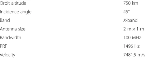
To verify the effectiveness of the modified method, com-puter simulations are given in this section. Experimental results are obtained based on 200 trials. The simulated DSS-SAR system in the side-looking mode is composed by seven satellites and all the satellites distribute uni-formly with the antenna spacing l=vsTr/M (Tr is the pulse repetition period) in the along-track direction [9,12]. The other parameters are listed in Table 1. The gain, phase, and position errors for each of the M

satellites, i.e., gm, ξ0m, and Δxm, are defined as uniform random variables in [1−α, 1 +α], [−π, π], and [−Δp, Δp], respectively. They are generated and maintained in-variant in each trial. The average root mean squared error (ARMSE) of gain, phase, and position errors are

defined as 1 M1

XM

m¼2

RMSEf ggm , _M1₁

XM

m¼2

RMSEfξ0mg ,

1 M1

XM

m¼2

RMSEfΔxmg, respectively.L andL0are set to be

10 and 3, respectively. The Doppler frequencyfdis fixed to be zero.

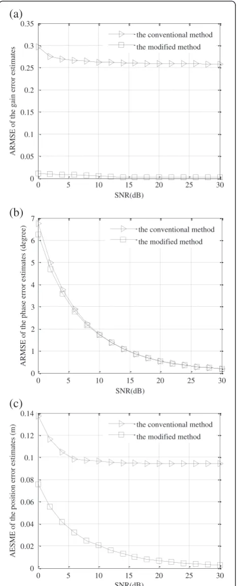
3.1. Effect of SNR

Suppose Δp= 0.25l and α= 0.2. The ARMSE curves of gain, phase, and position error estimates versus signal-to -noise ratio (SNR) are shown in Figure 2a–c, respect-ively. From Figure 2, it is observed that both the modi-fied method and the conventional method perform better as the SNR increases. From Figure 2a,c, it can be seen that gain and position error estimation performances of the conventional method are worse than those of the modified method. It is because gain

Table 1 Simulation parameters of DSS-SAR systems

Orbit altitude 750 km

Incidence angle 45°

Band X-band

Antenna size 2 m × 1 m

Bandwidth 100 MHz

PRF 1496 Hz

and position error estimations cannot be separated in the conventional method and they interfere with each other. However, in the modified method, because gain errors are corrected before estimating position errors, position error estimates can converge to optimal solutions. The position error estimate ARMSE is lower than 0.01 m when the SNR is larger than 15 dB. In addition, it is shown in Figure 2b that phase error estimations can work well for both methods. This is consistent with the analysis in modified method for DSS-SAR system, which shows that position errors have no influence on the phase error estimation when the zero Doppler bin is chosen. However, the computational load of the modified algorithm is lower than the conven-tional method.

0 5 10 15 20 25 30

0 0.05 0.1 0.15 0.2 0.25 0.3 0.35

SNR(dB)

ARMSE of the gain error estimates

the conventional method

the modified method

(a)

0 5 10 15 20 25 30

0 1 2 3 4 5 6 7

SNR(dB)

ARMSE of the phase error estimates (degree)

the conventional method

the modified method

(b)

0 5 10 15 20 25 30

0 0.02 0.04 0.06 0.08 0.1 0.12 0.14

SNR(dB)

AESME of the position error estimates (m)

the conventional method

the modified method

(c)

Figure 2ARMSE of gain, phase and position error estimates versus SNR. (a)ARMSE of gain error estimates versus SNR;(b)

ARMSE of phase error estimates versus SNR;(c)ARMSE of position error estimates versus SNR.

0 0.1 0.2 0.3 0.4

0.53 0.535 0.54 0.545 0.55 0.555 0.56 0.565 0.57

ARMSE of the phase error estimates (degree)

ARMSE of the position error estimates (degree)

before gain error calibrated

after gain error calibrated

(a)

0 0.1 0.2 0.3 0.4

0 0.05 0.1 0.15 0.2 0.25 0.3 0.35

before gain error calibrated

after gain error calibrated

(b)

0 0.07 0.14 0.21 0.28 0.35 0.42 0.49 0

1 2 3 4 5 6 7 8

p ( antenna spacing l units)

ARMSE of the gain error estimates

the conventional method

the modified method

(a)

0 0.07 0.14 0.21 0.28 0.35 0.42 0.49 0

10 20 30 40 50 60

p ( antenna spacing l units)

ARMSE of the phase error estimates (degree)

the conventional method

the modified method

(b)

0 0.07 0.14 0.21 0.28 0

0.2 0.4

0 0.07 0.14 0.21 0.28 0.5

0.55 0.6

0 0.07 0.14 0.21 0.28 0.35 0.42 0.49 0

2 4 6 8 10 12

p ( antenna spacing l units)

ARMSE of the position error estimates (m)

the conventional method

the modified method

(c)

0 0.07 0.14 0.21 0.28 0

0.1 0.2

Figure 4ARMSE of gain, phase and position error estimates versue position error. (a)ARMSE of gain error estimates versus position error;(b)ARMSE of phase error estimates versus position error;(c)ARMSE of position error estimates versus position error.

2 4 6 8 10

0.25 0.26 0.27 0.28 0.29 0.3 0.31

number of iterations

A

R

M

S

E o

f th

e g

ain

er

ro

r es

timaties

the conventional method (a)

2 4 6 8 10

0.5445 0.545 0.5455 0.546 0.5465 0.547

number of iterations

ARMSE of the phase erroe of estimates (degree)

the conventional method (b)

2 4 6 8 10

0 0.02 0.04 0.06 0.08 0.1 0.12

number of iterations

ARMSE of the position error estimates (m)

the conventional method

the modified method (c)

3.2. Effect of gain errors

In the simulation, α changes from 0 to 0.4. Δp= 0.25l. SNR is 20 dB. The other parameters in the simulation are the same as the former. The effect of gain estimation errors on the following phase and position error estimations in the modified method is given in Figure 3, where the curve gained without calibrating gain errors is denoted as “before gain error calibrated” while the other curve named “after gain error calibrated” is obtained by calibrating gain errors first. It can be seen that if gain errors cannot be well calibrated, the position error estima-tion difference becomes larger with the increment of α, while the change of phase error estimation can be ignored. By using the modified method, both of phase and position error estimations can work well. It is clear that gain errors have serious influence on the following position error esti-mation and it is necessary to estimate gain errors first.

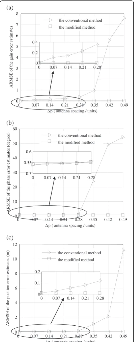
3.3. Effect of position errors

Fixing SNR to 20 dB. α= 0.2. ARMSE curves of gain, phase, and position error estimates versus position error are shown in Figure 4a–c, respectively. Local simulation results (small figures embedded in Figure 4) are also given for better explanation. Being consistent with the analysis in modified method for DSS-SAR system, gain and position error estimations interfere with each other, which make gain and position error estimations con-verge to suboptimal solutions in the conventional method. So, the estimation accuracy of the conventional method cannot satisfy the requirement. The gain error estimate ARMSE is larger than 0.1 while the position error estimate ARMSE is close to 0.03 whenΔp= 0.07l. In addition, phase error estimates obtained by both of the conventional method and the modified method are approximately equal to each other whenΔp≤0.28l. This is consistent with the previous analysis. By using the data of the zero Doppler bin, phase errors can be estimated with existing position errors. However, when Δp≥0.35l, the conventional method fails to work since gain and position error estimates deviate badly from the true values which has a strong impact on the phase error estimation.

3.4. Effect of iterations

Fix α= 0.2, Δp= 0.25l and suppose SNR to be 20 dB. The gain, phase, and position error estimation perform-ance of the conventional method versus the number of iterations is shown in Figure 5a–c, respectively. It is observed from Figure 5a,c that the conventional method converges slowly and even to suboptimal solutions since gain and position error estimations can interact with each other. However, it is noticed from Figure 5b that the phase error estimation can work well as we analyzed before.

For the modified method, only the position error esti-mate ARMSE versus the number of iterations is shown in Figure 5c since only the position error estimation is iterated in the modified method. It is noticed from Figure 5c that the position error estimation converges to the optimal solution with less than three iterations. To sum up, the computational load of the modified method is less than that of the conventional method. Meanwhile better performance can be obtained by the modified method.

4. Conclusions

In this study, we focus on gain, phase, and position error estimations of DSS-SAR systems. Based on the conven-tional method, a modified array error estimation method is proposed here. In the conventional method, the esti-mation of gain and position errors may converge to sub-optimal solutions especially when position errors are large and the joint iteration between the gain-phase and position error estimations are needed. That is because of the interaction between the estimations of gain and pos-ition errors. In the modified method, gain errors are first estimated and compensated before the other errors’ esti-mation, which guarantees the position error estimation accuracy to be higher than that in the conventional method. Meanwhile, by using the zero Doppler bin data, the phase error estimation can behave independently of position errors. Then the joint iteration strategy between the gain-phase and position error estimations in the conventional method can be avoided, which makes the modified method perform stably with low computational load. Theoretical analysis and simulation results demon-strate the effectiveness of the modified method.

Competing interests

The authors declare that they have no competing interests.

Acknowledgment

The authors would like to thank the anonymous reviewers for their constructive comments, which led to significant improvements in this study. Special thanks to Dr. Yinghua Wang and Xuefeng Zheng for improving the English usage and also for their valuable suggestions. This study was sponsored in part by the National Basic Research Program of China (973 Program) under Grant no. 2011CB707001, in part by the Natural Science Foundation of China under Grant no. 61101242, in part by the Fundamental Research Funds for the Central Universities under Grant no. K50511020009, and in part by the Program for Changjiang Scholars and Innovative Research Team in University under Grant no. IRT0954.

Received: 19 June 2012 Accepted: 7 December 2012 Published: 22 February 2013

References

1. D Zhen, C Bin, L Diannong, Detection of ground moving targets for two-channel spaceborne SAR-ATI. EURASIP J. Adv. Signal Process., Article ID 230785 (2010). doi:10.1155/2010/230785

2. F Lombardini, M Pardini, G Fornaro et al, Linear and adaptive spaceborne three-dimensional SAR tomography: a comparison on real data. IET Radar Sonar Navigat.3(4), 424–436 (2009)

4. S Chiu, MV Dragosevic, Moving target indication via RADARSAT-2 multichannel synthetic aperture radar processing. EURASIP. J. Adv. Signal Process., (2010). doi:10.1155/2010/740130

5. K Tomiyasu, Image processing of synthetic aperture radar range ambiguous signals. IEEE Trans. Geosci. Remote Sens.32(5), 1114–1117 (1994) 6. NA Goodman, SC Lin, D Rajakrishna, JM Stiles, Processing of multiple

receiver, spaceborne arrays for wide-area SAR. IEEE Trans. Geosci. Remote Sens.40(4), 841–852 (2002)

7. S Li, HP Xu, LQ Zhang, An advanced DSS-SAR InSAR terrain height estimation approach based on baseline decoupling. Prog. Electromagn. Res.

119, 207–224 (2011)

8. CH Gierull, D Cerutti-Maori, J. Ender, Ground moving target indication with tandem satellite constellations. IEEE Geosci. Remote. Sens. Lett.5(4), 710–714 (2009) 9. JP Aguttes, The SAR train concept: required antenna area distributed over N

smaller satellites, increase of performance by N, inProceedings of the IGARSS’03, Toulouse, France(, 2003), pp. 542–544

10. ZF Li, HY Wang, T Su, Z Bao, Generation of wide-swath and high-resolution SAR images from multichannel small spaceborne SAR Systems. IEEE Geosci. Remote. Sens. Lett.2(1), 82–86 (2005)

11. Z Lei, Q Cheng-Wei, X Mengdao, B Zheng, SAR imaging and Doppler ambiguity removal with distributed microsatellite arrays. Int. J. Remote. Sens.

31(24), 6441–6458 (2010)

12. ZF Li, Z Bao, HY Wang, GS Liao, Performance improvement for constellation SAR using signal processing techniques. IEEE Trans. Aerosp. Electron. Syst.

42(2), 436–451 (2006)

13. AJ Weiss, B Friedlander, DOA and steering vector estimation using a partially calibrated array. IEEE Trans. Aerosp. Electron. Syst.32(3), 1047–1057 (1996) 14. KV Stavropoulos, A Manikas, Array calibration in the presence of unknown

sensor characteristics and mutual coupling, inProceedings of the EUSIPCO, Toulouse, France(, 2000), pp. 1417–1420

15. L Aifei, L Guisheng, Z Cao et al, An eigenstructure method for estimating DOA and sensor gain-phase errors. IEEE Trans. Signal Process.

59(12), 5944–5956 (2011)

16. B Friedlander, AJ Weiss, Direction finding in the presence of mutual coupling. IEEE Trans. Antennas Propagat.39(3), 273–284 (1991) 17. AJ Weiss, B Friedlander, Array shape calibration using sources in unknown

locations-a maximum likelihood approach. IEEE Trans. Acoust. Speech Signal Process.37(12), 1958–1966 (1989)

18. MP Wylie, S Roy, RF Schmitt, Self-calibration of linear equi-spaced (LES) arrays, inProceedings of the ICASSP-93, Minneapolis, USA(, 1993), pp. 281–284

doi:10.1186/1687-6180-2013-31

Cite this article as:Xuet al.:Self-calibration method without joint iteration for distributed small satellite SAR systems.EURASIP Journal on Advances in Signal Processing20132013:31.

Submit your manuscript to a

journal and benefi t from:

7 Convenient online submission 7 Rigorous peer review

7 Immediate publication on acceptance 7 Open access: articles freely available online 7 High visibility within the fi eld

7 Retaining the copyright to your article