R E S E A R C H
Open Access
Unified tensor model for space-frequency
spreading-multiplexing (SFSM) MIMO
communication systems
André LF de Almeida
1*and Gérard Favier
2Abstract
This paper presents a unified tensor model for space–frequency spreading-multiplexing (SFSM) multiple-input multiple-output (MIMO) wireless communication systems that combine space- and frequency-domain spreadings, followed by a space–frequency multiplexing. Spreading across space (transmit antennas) and frequency (subcarriers) adds resilience against deep channel fades and provides space and frequency diversities, while orthogonal
space–frequency multiplexing enables multi-stream transmission. We adopt a tensor-based formulation for the proposed SFSM MIMO system that incorporates space, frequency, time, and code dimensions by means of the parallel factor model. The developed SFSM tensor model unifies the tensorial formulation of some existing
multiple-access/multicarrier MIMO signaling schemes as special cases, while revealing interesting tradeoffs due to combined space, frequency, and time diversities which are of practical relevance for joint symbol-channel-code estimation. The performance of the proposed SFSM MIMO system using either a zero forcing receiver or a semi-blind tensor-based receiver is illustrated by means of computer simulation results under realistic channel and system parameters.
Keywords: Blind receiver, MIMO–OFDM communications, Parallel factor analysis, Space–frequency spreading-multiplexing, Tensor modeling
1 Introduction
Wireless communication systems employing multiple antennas at both ends of the link, commonly known as multiple-input multiple-output (MIMO) systems, are being considered as one of the key technologies to be deployed in current and upcoming wireless com-munication standards [1]. In this context, the inte-gration of multiple-antenna systems with code-division multiple-access (CDMA) transmission and/or orthogo-nal frequency division multiplexing (OFDM) has also been the subject of several works over the past few years [2-4].
Different combinations of OFDM and CDMA have been reported in a number of works. Multi-carrier (MC)-CDMA performs spreading of the information symbols across the different subcarriers [5,6], but suffers from lim-ited frequency diversity gains like conventional CDMA
*Correspondence: [email protected]
1Department of Teleinformatics Engineering, Federal University of Ceará, Fortaleza, Brazil
Full list of author information is available at the end of the article
systems. MC direct-sequence (MCDS)-CDMA differs from MC-CDMA by performing the spreading operation in the time-domain at each subcarrier [7]. For combat-ing frequency-selective fadcombat-ing, MCDS-CDMA requires forward error-correction coding and frequency-domain interleaving. In [8], a hybrid of MC-CDMA and OFDM systems with orthogonal transmission in the frequency-domain was proposed, which ensures interference-free transmission/reception regardless of the multipath chan-nel profile. A related approach, called multicarrier block-spread (MCBS)-CDMA, was introduced in [9] by cap-italizing on redundant block spreading and frequency-domain linear precoding to preserve orthogonal multiple-accessing and to enable full multipath diversity gains. The receiver is based on a low-complexity single-user equalization.
By introducing the spatial dimension at the trans-mit processing, jointly with time and/or frequency dimensions, a number of different space–frequency MIMO transceivers were proposed to enable orthogonal multiple-access in multiuser systems combining OFDM
and CDMA techniques. A spread spectrum-based trans-mission framework was proposed in [10], therein called multicarrier spread space spectrum multiple access (MC-SSSMA), with the idea of fully spreading each user symbol over space, time, and frequency. MC-SSSMA is a gen-eralization of its single-carrier counterpart proposed in [11]. Despite the achieved spectral efficiency gains, the design of [10] was restricted to the case where the number of transmit and receive antennas is equal to the spread-ing gain. In [12], space–time–frequency spreadspread-ing was proposed for MC-CDMA based on the concatenation of a space–time spreading code with a frequency-domain spreading code.
A common characteristic of all these works is the assumption of perfect channel knowledge at the receiver. When the channel is not known, as it is the case in practice, the receiver design is generally based on subop-timum (linear or nonlinear) filtering/equalization/signal separation structures that use training sequences for channel acquisition and tracking, before decoding the transmitted data. However, practical limitations such as the receiver complexity and the training sequence overhead (which implies a reduction of the informa-tion rate) may be too restrictive and prohibitive in some cases.
Recently, tensor modeling has successfully been applied to the design of MIMO transceivers based on spatial mul-tiplexing and/or space–time coding [13-19]. Relying on the use of spreading codes, the common feature of these works is the fact that the received signal can be mod-eled as a third-order tensor, the dimensions of which are associated withspace,time, andcodediversities [20]. Due to the uniqueness properties of tensor models, these tensor-based MIMO–CDMA transceivers afford blind multiuser detection and channel estimation under more relaxed conditions compared with conventional matrix-based receivers. The approach of [13] relies on pure spatial multiplexing by means of a parallel factor (PARAFAC) model [21]. The work of [14] deals with a multiple-access MIMO antenna system relying on a block tensor model [22]. In [15], a constrained “block-structured” PARAFAC model is proposed for allowing multiuser space–time spreading in the uplink. The multiuser downlink case is treated in [16]. More general tensor-based space–time spreading and multiplexing structures were also pro-posed relying on the constrained factor (CONFAC) model [17,18] and on PARATUCK-type models [19,23].
In this article, we present a unified tensor model for space–frequency spreading-multiplexing (SFSM) MIMO wireless communication systems combining both space and frequency spreadings along with a space–frequency multiplexing. On one hand, spread-ing across space (transmit antennas) and frequency (subcarriers) potentially provides robustness against
frequency-selective fading and channel ill-conditioning while providing transmit diversity gains. On the other hand, an orthogonal space–frequency multiplexing enables interference-free multistream transmission. For this system, we adopt a tensorial formulation of the transmitted and received signals that jointly incorpo-rates space, frequency, time, and code dimensions by means of a PARAFAC tensor model. From this tensorial formulation, we show how several existing multiple-antenna CDMA-based systems can be derived by making appropriate simplifications on the unified tensor model structure.
We also address the problem of joint symbol-channel-code estimation for the proposed system by capitalizing on the uniqueness properties of the PARAFAC model. By exploiting the space, time, frequency, and code diversi-ties inherent to the unified SFSM tensor model, we obtain new results providing useful bounds on the required number of transmit and receive antennas, subcarriers, and spreading length for ensuring a unique recovery of users’ symbols, channels, and codes. A performance eval-uation of the SFSM MIMO system is also carried out considering a zero forcing (ZF) receiver and a semi-blind alternating least squares (ALS) receiver that only requires a single pilot symbol per transmitted data stream in order to remove the scaling factor introduced by the estimation process.
The remainder of this article is organized as follows. In Section 2, the main building blocks of the SFSM trans-mitter are detailed and the transmitted signal model is formulated. In Section 3, we present the received signal model and also derive the proposed unifying tensor model and its special cases. A ZF receiver with joint block-decoding and equalization is formulated in Section 4. Section 5 is dedicated to the problem of joint symbol-channel-code estimation for the unified SFSM MIMO system, where bounds on the required numbers of trans-mit/receive antennas, subcarriers, spreading length, and the number of symbols per data stream are provided. The semi-blind ALS receiver is also presented in this section. In Section 6, the performance of the SFSM MIMO system is evaluated by means of computer simulations under dif-ferent system parameter settings. The article is concluded in Section 7.
Notations: Some notations and properties are now defined. Scalars are denoted by lower-case letters (a,b,. . .), vectors are written as boldface lower-case let-ters (a,b,. . .), matrices as boldface capitals (A,B,. . .), and tensors as calligraphic letters (A,B,. . .). We use ai,j =[A]i,j to denote the entry (i,j) of matrix Awhile ai,j,k,l refers to the entry (i,j,k,l) of the tensor A ∈
CI×J×K×L. Theith row andjth column ofAare denoted
A† stand for transpose, inverse, and pseudo-inverse of
A, respectively. The operator diag(·) forms a diagonal matrix from its vector argument, whileblockdiag(·)forms a block-diagonal matrix from its matrix arguments. The operatorvecdiag(·)forms a column vector out of the main diagonal of its matrix argument, while1Rdenotes the
“all-ones” vector of dimensionR. The operator vec(·) forms a vector by stacking the columns of its matrix argument. Di(A)forms a diagonal matrix holding theith row ofA
on its main diagonal. The Kronecker and the Khatri-Rao products are denoted by⊗and, respectively:
AB=[A·1⊗B·1,. . .,A·R⊗B·R]= ⎡ ⎢ ⎣
BD1(A)
.. .
BDI(A) ⎤ ⎥
⎦∈CIJ×R
(1)
withA =[A·1. . .A·R]∈ CI×R,B =[B·1. . .B·R]∈ CJ×R.
We shall make use of the following properties of the Khatri-Rao product:
vec
Adiag(x)BT =(BA)x, (2)
withA∈CI×R,B∈CJ×Randx∈CR, and
(AB)H(AB)=AHA∗BHB, (3)
where ∗ denotes the Hadamard (element-wise) matrix product.
2 SFSM: transmitted signal model
We consider the uplink of a single-cell multicarrier mul-tiuser MIMO system with Q active co-channel users transmitting data across the same set of F subcarriers. Each user terminal is equipped withMttransmit
anten-nas and transmits R data streams. The base station is equipped withMrreceive antennas. The proposed SFSM
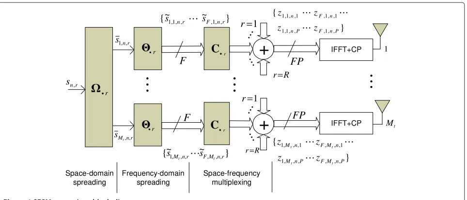
transmission structure is composed of three main oper-ations: (i) space spreading, (ii) frequency spreading, and (iii) space–frequency block-coding. Figure 1 depicts the block diagram of the transmitter structure by focusing on the transmission of thenth symbol of therth data stream. For notational simplicity, we begin by limiting ourselves to a single-user transmission model in order to facilitate the presentation. Later on, we show that the multiuser signal model is readily obtained with minor changes in notation.
2.1 Space-domain spreading
The input symbol sequence is serial-to-parallel converted intoRdata streams, each one being constituted byN sym-bols. For thenth symbol period, let us definesn,r as the nth symbol of therth data stream. The first operation is the space spreading, which consists in spreading each data
stream on theMttransmit antennas using a different code.
Let us define =.[·1,. . .,·r,. . .,·R]∈CMt×Ras the
matrix collecting the code vectors of theRdata streams. The space-domain spread signal is defined by the third-order tensorS¯ ∈ CMt×N×R, the (m
t,n,r)th element of
which is given by
¯
smt,n,r=ωmt,rsn,r, (4)
and represents thenth space spread symbol of therth data stream transmitted by themtth antenna.
For the space-domain spreading matrix, we choose a Vandermonde design with complex generatorsρmt =
e−j2π(mt−1)/max(Mt,R),m
t=1,. . .,Mt, i.e.
(ρ1,. . .,ρMt)=. √1 Mt
⎡ ⎢ ⎢ ⎢ ⎣
1 1 · · · 1 1 ρ2 · · · ρ2R−1
..
. ... · · · ... 1 ρMt · · · ρ
R−1 Mt
⎤ ⎥ ⎥ ⎥
⎦. (5)
As shown in [24], the Vandermonde structure mini-mizes an upper bound of the pairwise error probability at high signal-to-noise ratios (SNRs). Moreover, this struc-ture yields a good coding gain and makes the transmis-sion more robust to ill-conditioned/rank-deficient MIMO channels [25].
2.2 Frequency-domain spreading
The second operation consists in jointly spreading and coding each component¯smt,n,r in the frequency-domain.
This operation is implemented by means of linear precod-ing, which adds transmit redundancy in the frequency-domain before the multicarrier modulation. Each data symbol is transmitted simultaneously (in parallel) on dif-ferent subcarriers in a way similar to an MC-CDMA system with frequency-domain spreading [26]. In addition to provide frequency diversity gains, frequency-domain spreading adds resilience to symbol detection even in the presence of a deep channel fade over one or more subcarrier channels.
Let =.[·1,. . .,·r,. . .,·R]∈ CF×R be the
fre-quency spreading matrix. The output of this frefre-quency spreading operation is given by
˜
sf,mt,n,r =θf,r¯smt,n,r =θf,rωmt,rsn,r, (6)
which is the(f,mt,n,r)th element of the fourth-order
ten-sor S˜ ∈ CF×Mt×N×R representing the space–frequency
spread signalsn,r associated with thenth symbol period
Figure 1SFSM transmitter block-diagram.
The frequency spreading can be redundant (F > R) or not (F ≤R). As for the space-domain spreading, here we also choose as a Vandermonde matrix with complex generatorsνf =e−j2π(f−1)/max(F,R),f =1,. . .,F, i.e.
(ν1,. . .,νF)=.
1
√ F
⎡ ⎢ ⎢ ⎢ ⎣
1 1 · · · 1 1 ν2 · · · ν2R−1
..
. ... · · · ... 1 νF · · · νFR−1
⎤ ⎥ ⎥ ⎥
⎦. (7)
The reason for choosing the Vandermonde structure for the frequency spreading matrix follows that of the space spreading matrix. Some designs forhave been reported in the literature (we refer the interested reader to [27] for further details).
Note that spreading in the space-domain consists in multiplying the symbol sn,r by a complex code that
depends on the transmit antenna number mt while
spreading in the frequency-domain results in a multiplica-tion of the same symbol by a complex code that depends on the frequency numberf, as shown in (6).
2.3 Space-frequency multiplexing
The third operation of the SFSM transmitter consists in a multiplexing of theRspace–frequency spread sym-bols. Using conventional direct sequence (DS) spread-ing, each space–frequency symbol ˜sf,mt,n,r is spread by
a factor P using a specific spreading code. Due to spectrum spreading at the subcarrier level, each sub-carrier signal constitutes a DS spread signal. Conse-quently, the frequency spectrum associated with each subcarrier is allowed to overlap in order to achieve high spectral efficiency.
Denote C =.[C·1,. . .,C·r,. . .,C·R]∈ RP×R as the
spreading code matrix the columns/rows of which belong to a (possibly truncated) Walsh–Hadamard (WH) code matrix. WhenP ≤ R, we formCby selecting thePfirst rows of anR×RWH matrix. Each spreading code vec-tor is applied with the chip period Tc = T/P, where T corresponds to the OFDM symbol duration. The pro-posed space–frequency multiplexing operation consists in summing up RDS spread signals, each one of which being obtained by multiplying˜sf,mt,n,rby the
correspond-ing spreadcorrespond-ing codecp,r. Therefore, this operation yields a
multi-stream signal tensorZ∈CF×Mt×N×Pwhose typical
element is given by
zf,mt,n,p=
R
r=1 ˜
sf,mt,n,rcp,r. (8)
2.4 Multicarrier modulation
Before being transmitted, the space–frequency multi-plexed signal passes through the OFDM modulator. Con-sidering a frequency selective wireless link between each transmit-receive antenna pair, define Lmax as the
maxi-mum length of the impulse response of all the channels, including the effects of the physical channel, and pre-/post-filtering at transmitter and receiver. An inverse fast Fourier transform (IFFT) is applied and a cyclic prefix (CP) of Lmax chips is appended to the resulting
time-domain samples. Let = TcpFH ∈ CJ×F be a matrix representing the combined IFFT and CP-adding opera-tion, where F ∈ CF×F is an FFT matrix, with [F]k,f = e−j2π(k−1)(f−1)/F, Tcp =[ITcp,IF]T ∈ CJ×F is the
CP-adding matrix,J=F+Lmax, andIcpis the matrix formed
F. The output of the IFFT+CP-adding block correspond-ing to the transmitted signal is given by the followcorrespond-ing tensor transformation:
xj,mt,n,p=
F
k=1
ξj,kzk,mt,n,p, j=1,. . .,J. (9)
whereξj,k =[]j,k andxj,mt,n,pis a typical element of the
transmitted signal tensorX ∈CJ×Mt×N×P.
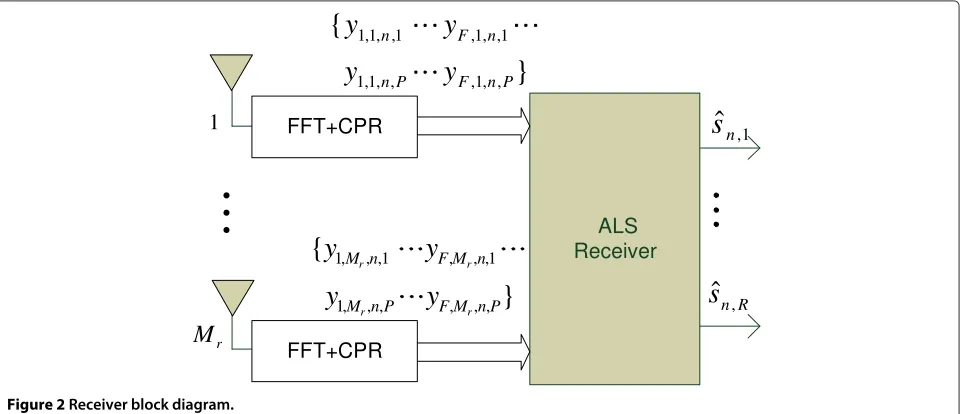
3 SFSM: received signal model
The block diagram of the receiver is depicted in Figure 2. We adopt a discrete-time baseband equivalent model for the received signal in the SFSM MIMO system, assum-ing perfect chip- and symbol-level synchronization at the receiver. Following the tensor notation used in the pre-vious section, the fourth-order tensor V ∈ CJ×Mr×N×P
representing the time-domain received signal in absence of noiseais defined as:
vj,mr,n,p=
Mt
mt=1
J
j=1 ˙
hj−j,mr,mtxj,mt,n,p
= Mt
mt=1
F
k=1 J
j=1 ˙
hj−j,mr,mtξj,kzk,mt,n,p, (10)
whereh˙j,mr,mt is an element of the tensorH˙ ∈CJ×Mr×Mt,
˙
H·mrmt ∈ CJ×1being the impulse response of the
chan-nel linking themrth receive antenna to themtth transmit
antenna.
The time-domain samples vj,mr,n,p pass through the
combined FFT and CP-removal (CPR) block, represented here by¯ = FRcp ∈ CF×J, whereRcp =[0F×Lmax,IF]∈
CF×Jis the CPR matrix. This yields the following received
signal tensorY∈CF×Mr×N×P:
yf,mr,n,p=
J
j=1 ¯
ξf,jvj,mr,n,p. (11)
Using (10), we can rewrite (11) as
yf,mr,n,p=
Mt
mt=1
F
k=1 ⎛ ⎝J
j=1 J
j=1 ¯
ξf,jh˙j−j,mr,mtξj,k
⎞ ⎠
hf,k,mr,mt
zk,mt,n,p,
(12)
where hf,k,mr,mt corresponds to the end-to-end
(frequency-domain) channel tensor H ∈ CF×F×Mr×Mt
that results from the combined FFT+CPR and IFFT+CP transformations at the receiver and transmitter, respec-tively. Note thathf,k,mr,mt is zero for allf = k. In matrix
notation, this can be seen by noting that the matrix slice
¨
H··mr,mt ∈CF×FofH¨, defined by [H¨··mr,mt]f,k
.
=hf,k,mr,mt,
has a diagonal structure [28]. Consequently, we can sim-plify (12) by eliminating the summation over index k, yielding
yf,mr,n,p=
Mt
mt=1
hf,f,mr,mtzf,mt,n,p. (13)
Finally, using (6) and (8), we can rewrite (13) as:
yf,mr,n,p=
Mt
mt=1
R
r=1
hf,f,mr,mtθf,rωmt,rsn,rcp,r. (14)
In the next section, we show how the tensor model (14) satisfied by the received signals can be cast into a PARAFAC model by contracting the first two modes of
the transmitted and received signal tensors. Our motiva-tion behind the use of PARAFAC modeling comes from the possibility of studying identifiability by resorting to the well-known results available in the literature.
3.1 PARAFAC model formulation
In its general form, the PARAFAC decomposition amounts to decomposing the third-order tensor X ∈ CI1×I2×I3 into a sum ofR rank-one third-order tensors [21]. It has the following scalar representation
xi1,i2,i3 =
R
r=1 a(i1)
1,ra
(2) i2,ra
(3)
i3,r (15)
wherea(inn,)ris the entry(in,r)of thenth mode matrix factor A(n) ∈CIn×R,n= 1, 2, 3. WhenRis minimal, it is called
the rank ofX.
Starting from the space–frequency block-coded signal (8), let us contract the first two modes of the coded sig-nal tensor Z ∈ CF×Mt×N×P as m = (f −1)M
t+ mt,
withM=FMt, and define the space–frequency spreading
matrixU∈CM×Rsuch as
um,r=ωmt,rθf,r↔U·r=·r·r↔U=.
(16)
Then, Equations (6), (8), and (16) lead to the following contracted signal tensor:
¯ zm,n,p=
R
r=1
um,rsn,rcp,r, (17)
which corresponds to a third-order PARAFAC model for the transmitted signal tensorZ¯ ∈ CM×N×P, with matrix
factors(U,S,C).
Following the same reasoning, let us now contract the first two modes of the received signal tensor Y ∈ CF×Mr×N×P by defining i = (f − 1)M
r + mr, with I =FMr. Combining this contraction with the one
intro-duced for the transmitted signal tensorZ¯ ∈CM×N×Pand using (17), we get the following contracted received signal tensorY¯ ∈CI×N×P:
¯ yi,n,p=
M
m=1 ¯
hi,mz¯m,n,p= R
r=1 M
m=1 ¯
hi,mum,rsn,rcp,r, (18)
where H¯ ∈ CI×M is a channel matrix obtained from a double contraction of the end-to-end chan-nel tensor H ∈ CF×F×Mr×Mt such as [H¯]
i,m=
[H¯](f−1)Mr+mr=h(f−1)Mt+mr= hf,f,mr,mt. Defining G ∈
CI×R with element g i,r =
M m=1
¯
hi,mum,r as the effective
MIMO channel linking the R multiplexed data streams
at the transmitter to the I = FMr equivalent
subchan-nel outputs at the receiver, the tensorY¯ can be rewritten element-wise as
¯ yi,n,p=
R
r=1
gi,rsn,rcp,r, (19)
which corresponds to a third-order PARAFAC model for the contracted received signal tensorY¯. The final step is to determine an adequate expression for the factorization of the effective MIMO channel matrixG. From the definition ofgi,rand the expression (16) ofU, we get
G= ¯HU= ¯H()∈CI×R. (20)
Note that the contracted received signal tensor Y¯ ∈ CI×N×P given by (19) follows a PARAFAC model with
matrix factors (H¯( ), S, C). In fact, models (17) and (19) for the transmitted and received signal tensors, respectively, differ only in their first-mode matrix factors, which are related by (20).
For the model (19), we have the following matrix repre-sentations:
¯
Y1=(CG)ST ∈CPI×N, (21)
¯
Y2=(GS)CT ∈CIN×P, (22)
¯
Y3=(SC)GT ∈CNP×I, (23)
where [Y1¯ ](p−1)I+i,n=[Y2¯ ](i−1)N+n,p=[Y3¯ ](n−1)P+p,i= ¯
yi,n,p.
3.2 Multiuser case
The extension of the transmitted and received signal mod-els to the multiuser MIMO case is straightforward. Let us assume thatQusers are transmitting to the base sta-tion (uplink transmission) and that all users have the same numberMtof transmit antennas,Mr denoting the
num-ber of receive antennas at the base station. The multiuser signal model follows that of the single-user case by consid-ering a block-partitioned notation. In the multiuser case, the total number of transmitted data streams (summed over all the users) is equal toR=R(1)+ · · · +R(Q), where R(q)denotes the number of space–frequency spread data streams transmitted by the qth user. With these defini-tions, the received signal model (19) can be rewritten as follows
¯ yi,n,p=
Q
q=1 R(q)
r(q)=1 gi(,qr()q)s
(q) n,r(q)c
(q)
In this case, the mode-1 unfolded matrix representation of (24) is given by
¯
Y1=
Q
q=1
(C(q)G(q))S(q)T
=C(1)G(1),. . .,C(Q)G(Q)
⎡ ⎢ ⎣
S(1)T
.. .
S(Q)T
⎤ ⎥
⎦=(CG)ST,
(25)
whereS=[S(1),. . .,S(Q)]∈ CN×R,C=[C(1),. . .,C(Q)]∈ CP×R, G =[G(1),. . .,G(Q)]∈ CI×R. Therefore, the
PARAFAC model (17) is equally valid for the multiuser case by simply interpreting its factor matrices as block-matrices.
3.3 Special cases
The proposed structured PARAFAC model (19) of the received signal is general in the sense that it incorporates several existing multiple-access/multiple-antenna signal-ing schemes. By maksignal-ing appropriate assumptions, the proposed model can gradually be simplified, so that we obtain different tensor-based transceiver models as spe-cial cases:
• Space–time spreading CDMA (STS-CDMA) : For
F=1, which corresponds to a single-carrier transmission over a flat-fading channel, we can abandon the frequency-dependent index and
eliminate the frequency spreading matrix=1TR, so thatG= ¯H. Thus, the trilinear model (21) reduces to classical space–time spreading using multiple spreading codes and can be written as:
¯
Y1=(C ¯H)ST ∈CPMr×N. (26)
This model is valid for modeling the multiple-antenna transmission systems proposed in [25,29].
• Spatial multiplexing CDMA (SM-CDMA) : In
SM-CDMA systems, the space spreading operation (which is responsible for spreadingR data streams acrossMttransmit antennas) is eliminated. In other words, each data stream is transmitted by a different transmit antenna. Still consideringF=1, in this case we haveR=Mt,=IMt, and=1TR, which impliesG= ¯H, and model (21) becomes:
¯
Y1=(C ¯H)ST ∈CPMr×N. (27)
This model covers a spatial multiplexing/multiple-access CDMA system using a different spreading code per transmit antenna [2], and is the same as the PARAFAC-CDMA model proposed in the seminal paper [20]. It also coincides with the Khatri-Rao space–time (KRST) coding model of [13].
• Multicarrier CDMA systems (MCBS-CDMA
/MCDS-CDMA/ MC-CDMA) : We consider the transmission model of a MCDS-CDMA system where frequency-domain spreading and orthogonal multiplexing take place (e.g. see [26,30]). This is a single-input single-output (SISO) antenna system (Mr=Mt=1), which means that the channel matrixH¯ reduces to anF×Fdiagonal matrix, and we can eliminate the space spreading matrix=1TR so thatG= ¯H ∈CF×R. Consequently, the general PARAFAC model (21) becomes:
¯
Y1=(C ¯H)ST ∈CPF×N. (28)
It is worth noting that this special model can be interpreted as the tensorial formulation of the MCBS-CDMA system proposed in [9]. In particular, if frequency-domain spreading is not used, we have =IRso that (28) reduces to a PARAFAC model for a MCDS-CDMA system with direct-sequence spectrum spreading at the subcarrier level [7]. In the SISO case, whereH¯ ∈CF×Fis diagonal, if
space–frequency block-coding is not used (P=1and C=1TR), then (28) reduces to traditional
MC-CDMA, and we have:
¯
Y1= ¯HST ∈CF×N. (29)
• Conventional spatial multiplexing: This is the well-known single-user single-carrier MIMO system with spatial multiplexing (such as the V-BLAST system of [31]). Then, we haveF=P=1,R=Mt, andC==1TR,=IMt. In this case, the general
PARAFAC model (21) simplifies to the conventional matrix-based model:
¯
Y1= ¯HST ∈CMr×N. (30)
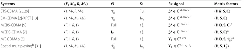
Table 1 summarizes the different special cases covered by the proposed tensor model. It allows us to deduce how the proposed tensor model parameters and the structure of the associated matrix factors are adjusted to model different existing systems in a tensorial form.
Table 1 Equivalent tensorial formulation for different systems
Systems (F,Mt,R,Mr) Rx signal Matrix factors
STS-CDMA [25,29] (1,Mt,R,Mr) 1TR Full Y∈CMr×N×P (H¯,S,C)
SM-CDMA [2]/KRST [13] (1,Mt,Mt,Mr) 1TR IMt Y∈CMr×N×P (H¯,S,C)
MCBS-CDMA [9] (F, 1,R, 1) Full 1T
R Y∈CF×N×P (H¯,S,C)a
MCDS-CDMA [7] (F, 1,R, 1) IR 1TR Y∈CF×N×P (H¯,S,C)a
MC-CDMAb [5] (F, 1,R, 1) Full 1T
R Y¯1∈CF×N (H¯,S,1TR)a
Spatial multiplexingb[31] (1,M
t,Mt,Mr) 1TR IMt Y¯1∈CMr×N (H¯,S,1TR)
aTensor models with diagonal channel matrixH¯∈CF×F.
bSystems in which the received signal model is reduced to a matrix (bilinear) decomposition.
subcarrier grouping in order to avoid unnecessary com-plicated mathematical notation in the formulation of the transmitted and received signal models.
4 ZF receiver
Assuming that the channel (H), code (C), and spread-ing (,) matrices are known at the receiver, we pro-pose a ZF receiver that simultaneously estimates all the R transmitted data streams by means of a joint block-decoding and an equalization without de-spreading. The ZF receiver is based on Equation (21). It minimizes the least squares (LS) criterion ¯Y1−(CG)ST2with respect to the symbol matrix, giving a simultaneous estimate of theRdata streams as:
ST =WY1¯ , (31)
where
W=(CG)†∈CR×PFMr. (32)
SinceCG ∈ CPFMr×Rmust be full column-rank to be
left-invertible, the ZF receiver requires thatPMrF≥R.
From the structure of (32), we can observe that the ZF receiver does not require code-orthogonality to jointly estimate the transmitted signals. In Section 5, we pro-pose a PARAFAC-based receiver that can blindly operate, i.e. without a priori knowledge of the space–frequency MIMO channel.
4.1 Space–frequency linear combiner
Note that, under the condition P ≥ R, the column-orthonormality of C turns the ZF receiver into a sim-pler space–frequency linear combiner that avoids matrix inversion and decodes each transmitted data stream sep-arately. Indeed, if C has orthonormal columns, we have
CHC = IR. By expandingWin (32) and using property
(3), we get
W=(CG)H(CG)−1(CG)H
=CHC∗GHG−1(CG)H
=(IR∗GHG)−1(CG)H
Since the Hadamard productIR∗GHGeliminates the
off-diagonal elements ofGHG, we have
W=
⎡ ⎢ ⎢ ⎢ ⎢ ⎢ ⎢ ⎣
GH·1G·1
γ1 . ..
GH·RG·R
γR
⎤ ⎥ ⎥ ⎥ ⎥ ⎥ ⎥ ⎦
−1
(CG)H, (33)
so that
ST·r= 1
γr(C·r⊗G·r)
HY1¯ , r=1,. . .,R. (34)
5 Semi-blind ALS receiver
The goal of the base station receiver is to separate the co-channel transmissions while recovering the data trans-mitted by each user. In our proposed SFSM MIMO sys-tem, co-channel transmissions are represented by theR data streams accessing simultaneously the space, time, and frequency channel resources. We are interested in a semi-blind receiver that neither requires prior knowledge, or estimation, of channel and antenna array responses, nor relies on statistical independence between the transmitted signals. These properties are distinguishing features of the PARAFAC modeling and constitute the main motivation for using the unified tensor model.
Moreover, the proposed receiver is called semi-blind in the sense that it relies only on a single pilot symbol inserted at the beginning of each data stream. This pilot symbol is used to remove the scaling factor introduced by the estimation process.
Let us rewrite the three unfolded matrices of the received signal in (21), (22), and (23), in the following manner
¯
Y1=Z(c,g)ST, Y¯2=Z(g,s)CT, Y¯3=Z(s,c)H¯T,
(35)
where Z(c,g) = C G ∈ CPFMr×R, Z(g,s) = G S ∈
CFMrN×R, and Z
(s,c) = (SC)()T ∈ CNP×FMt,
where we have used the factorization ofGdefined in (20). Identifiability of the symbol, code, and channel matrices in the LS sense from factorizations (35) requires thatZ(c,g), Z(g,s), andZ(s,c)be full column-rank, which implies
min(PFMr,FMrN)≥R, and NP≥R≥FMt. (36)
The first inequality comes from the full column-rank requirement ofCGandGS, while the second one comes from the full column-rank requirement of (S C)()T. These necessary conditions are useful when one is interested in eliminating system configurations leading to a non-identifiable model. We emphasize that conditions (36) do not imply model identifiability since it is not a sufficient condition.
In the following, we start from the Kruskal’s condition for the essential uniqueness of the PARAFAC decom-position [34] and then deduce simplified conditions by considering different special cases of practical interest. Directly applied to model (19), Kruskal’s condition states thatG,S, andCcan uniquely be estimated up to column permutation and scaling ambiguitiesb from the received data tensorY¯if
kG+kS+kC≥2R+2, (37)
wherek(·)denotes the Kruskal-rankcof a matrix.
Assume thatG = ¯HUis full rank. If the numberN of symbols is large enough compared to the numberRof data streams, the symbol matrixSis likely to be full rank. Note also that the space–frequency multiplexing matrixChas orthogonal columns and is full rank by definition. Taking these considerations into account, Kruskal’s condition can be written as [34,35]:
rank(G)+rank(S)+rank(C)≥2R+2. (38)
We now use the fact that G = ¯HU, with U given in (16) and consider particular cases leading to simpli-fications of (38) which are of practical relevance for the unified SFSM MIMO system. Interesting tradeoffs for joint symbol-channel-code estimation can explicitly be obtained.
5.1 Single-carrier transmission (F=1)
1. Mr≥Mt. We haveG= ¯H. Assuming thatH¯ is full column-rank andis full rank due to its
Vandermonde structure, it follows that
rank(G)=rank()=min(Mt,R), and (38) becomes:
min(Mt,R)+min(N,R)+min(P,R)≥2R+2.
(39)
2. R≥Mt. In this caseis full row-rank due to its Vandermonde structure. Assuming thatH¯ is modeled by i.i.d entries (which corresponds to scattering-rich propagation) and thus is full rank, it follows that rank(G)=rank(H¯)=min(Mr,Mt), which implies:
min(Mr,Mt)+min(N,R)+min(P,R)≥2R+2.
(40)
These two conditions (39) and (40) have interesting practical corollaries. Assuming that the number of sym-bols and the code spreading factors are large enough (i.e., bothS andC are full column-rank), they become, respectively,
min(Mt,R)≥2, (Mr≥Mt) (41)
and
min(Mr,Mt)≥2, (R≥Mt), (42)
and can be interpreted in the following way.
Corollary 1. For Mr ≥ Mt, spreading across Mt =
2 transmit antennas is sufficient for joint symbol-code-channel recovery, regardless of the numberR≥2 of data streams, for large enough number of symbols and code spreading factors.
Corollary 2. ForR ≥ Mt,Mr = 2 receive antennas are
sufficient for joint symbol-code-channel recovery, regard-less of the numberMt≥2 of transmit antennas, for large
enough number of symbols and code spreading factors.
5.2 Single-antenna transmission (Mt=1)
In this case,H¯ ∈ CFMr×F is full column-rank, and we
haveG= ¯H. Moreover, considering thatis full rank due to its Vandermonde structure, we have rank(G) = rank()=min(F,R), which implies:
min(F,R)+min(N,R)+min(P,R)≥2R+2. (43)
Now, assuming that S andC are full column-rank (i.e., N≥RandP≥R), condition (43) is equivalent to:
min(F,R)≥2 (44)
and we obtain:
Corollary 3. ForMt=1, spreading acrossF=2
subcar-riers is sufficient for joint symbol-code-channel recovery, regardless of the numberR≥2 of data streams, for large enough number of symbols and code spreading factors.
Note that this condition is independent on the number Mr of receive antennas, which means that joint
antenna. This clearly illustrates the tradeoff between fre-quency diversity and space diversity at the receiver, which is inherent to this trilinear PARAFAC model.
5.3 Small spreading lengths (P<R)
A different interpretation of (39) and (40) arises if S is full column rank, butP < R, i.e., the spreading length is smaller than the numberRof data streams. This is a chal-lenging situation, since most of the multiuser receivers (as well as the single-user one) needP≥Rin order to achieve multiuser interference rejection or de-spreading. In this case, for single-carrier transmissions (F = 1), conditions (39) and (40) reduce, respectively, to the following ones:
min(Mt,R)+P≥R+2, (45)
and
min(Mr,Mt)+P≥R+2. (46)
The simplified condition (45) results in the following corollary:
Corollary 4. ForMr ≥Mt ≥R, spreading acrossP = 2
chips is sufficient for joint symbol-code-channel recov-ery, regardless of the numberR ≥ 2 of data streams and receive antennas.
This condition establishes a tradeoff between code diversity (spreading length) and space diversity afforded by the proposed trilinear PARAFAC modeling.
Remark 2.When subcarrier grouping is used, receiver processing is parallelized into μ independent detection “layers”, each one associated withK = F/μsubcarriers. For this reason, identifiability can be studied group-wise (i.e., what matters for identifiability isK andnot F) since the results obtained for a given subcarrier group are equally valid for all the other groups.
It is worth mentioning that uniqueness conditions more relaxed than Kruskal’s one have been reported in [36,37], and can be applied to our PARAFAC model. For instance, it is common to assume that the symbol matrixSis full column-rank for sufficiently largeN. In this case, applying the sufficient condition derived in [37] to model (19) gives the following uniqueness condition:
PFMr(P−1)(FMr−1)≥2R(R−1). (47)
Note that this condition is more relaxed than Kruskal’s condition (37). In connection with [36], it is shown in [37] that this condition is valid ifGandCare randomly sampled from an(FMr+P)R-dimensional continuous
dis-tribution. In a recent work [38], a mathematical proof is provided to the case of non-randomGandCmatrices.
5.4 Receiver algorithm
The symbol-code-channel recovery is carried out by esti-mating each one of the three matrix factorsS,C, andGof the trilinear PARAFAC model (19) through the minimiza-tion of the following nonlinear cost funcminimiza-tion:
f(G,S,C)=
N
n=1 P
p=1 FMr
i=1 y¯i,n,p−
R
r=1
gi,rsn,rcp,r 2
. (48)
In this study, we propose the use of the ALS algorithm [20,39,40], which is the classical solution to minimize this cost function. It exploits the Khatri-Rao factoriza-tions (21)–(23) of the unfolded matrix representafactoriza-tions of the received signal tensor, by alternating among the esti-mation of G, S, and C. These estimates are found by, respectively, optimizing the three following LS criteria:
S=argmin
S
Y1−(CG)ST 2
F, (49)
C=argmin
C
Y2−(GS)CT2
F, (50)
G=argmin
G
Y3−(SC)GT2
F, (51)
where Yi = ¯Yi + Bi, i = 1, 2, 3, is the noisy
ver-sion of Y¯i, and Bi is a matrix representing the additive
complex-valued white Gaussian noise.dWe can rely on the knowledge of the space and frequency spreading matrices
and to directly obtain an LS estimate of H¯, pro-vided that the second inequality of (36) is satisfied, i.e.,
if R ≥ FMt. From (51), and using (20), we haveH¯ T
=
(SC)()T†Y3. On the other hand, ifR < FMt,
a unique estimation ofH¯ is not guaranteed, although we can still estimate S, C and G from (49), (50), and (51), respectively.
After convergence of the ALS algorithm, the estimated matrix factorsS,C, andH¯ are affected by unknown scaling factors. In order to eliminate the scaling ambiguity from the columns ofS, thus leading to an unambiguous sym-bol recovery, we assume that “all ones” pilot symsym-bols are introduced at the beginning of the transmission, i.e., at the first symbol of all the data streams. Mathematically speak-ing, this means that the first row of the symbol matrix is given byS1· =[ 1 1· · ·1]∈ C1×R. A final estimate of
the symbol matrix is therefore obtained in the following manner:
S=SD1(S) −1
,
whereD1(S)is the diagonal matrix formed from the first
row ofS.
In principle, the ALS receiver is capable of process-ing a higher number of users as long as condition (38) is satisfied. Regarding the computation complexity, three matrix inverses are performed at each iteration of the algorithm. The asymptotic complexity is thereforeO(R3)
per iteration. Consequently, a joint detection of a very large number of users can be prohibitive. This is gener-ally a common limitation of multiuser detection receivers. Note that the computational complexity can be reduced if users’ codes are mutually orthogonal. In this case, their symbol matrices can be estimated separately using (34).
6 Simulation results
We simulated a system operating at a transmission rate of Rc = 1/Tc = 4.096×10⁶chips per second (cps), using
a total ofF = 64 subcarriers divided intoμgroups ofK subcarriers each. Note thatF = 64 is a fixed parameter, whileK is a transmission design parameter (now repre-senting the frequency spreading length) that will be varied in our simulations. Due to subcarrier grouping, at each symbol period, Rsymbols belonging toR different data streams are transmitted usingμgroups ofKsubcarriers. In all simulations, we assume the transmission ofN =10 symbols per data stream. In order to avoid interference between adjacent subcarriers, a guard interval in the form of a CP is appended to each OFDM symbol [5]. Perfect time and frequency synchronization is assumed. Table 2 summarizes the SFSM MIMO system parameters.
Table 2 System parameters
Chip rate 4.096×10⁶cps
Number of subcarriers (F) 64
Number of subcarriers per group (K) 2 or 4
Number of subcarriers groups (μ) 32 or 16
CP length 5 (Chan. A)/20 (Chan. B)
Number of symbols per data stream (N) 10
Modulation QPSK
At each run, the transmitted symbols are randomly drawn from a quaternary phase shift keying (QPSK) alphabet. The channel is assumed quasi-static, which means that the channel impulse responses do not change during theNsymbol periods. Each plotted bit error rate (BER) curve is shown as a function of an overall SNR measure, given by
SNR=10 log10
Y2
F B2 F
whereB∈CF×Mr×N×Pis the additive noise tensor, whose
entries are circularly symmetric complex Gaussian ran-dom variables. Note that this SNR measure takes all the received signal dimensions into account, i.e., the number Fof subcarriers, the numberMr of receive antennas, the
number N of symbol periods, and the spreading length P. At each run, the additive noise power is generated according to this SNR measure. The BER curves represent the performance averaged over the R transmitted data streams and 1,000 independent Monte Carlo runs.
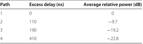
We adopt two frequency selective channel models for modeling the channel between each pair of transmit and receive antennas. Both are ITU’s outdoor-to-indoor mod-els, and are valid for typical urban propagation environ-ments: (i) the 4-ray pedestrian channel A and (ii) the 6-ray pedestrian channel B [44]. The channel parameters are summarized in Tables 3 and 4. Note that, for chan-nel A, the maximum multipath delay isτmax = 410 ns,
so that the maximum channel impulse response memory isLmax = τmax/Tc = 2 chip samples. We chose a CP
length of 5 chips when considering channel A. For chan-nel B, the maximum multipath delay isτmax = 3700 ns,
so that maximum channel impulse response memory has Lmax = τmax/Tc = 15 chip samples. We chose a CP
length of 20 chips when the channel B is simulated. In the following simulation results, the maximum num-ber of iterations allowed for the ALS algorithm is fixed to 1000. Thus, for each Monte Carlo run, we assume that the algorithm has converged at the tth iteration when
|e(t) −e(t−1)| < 10−4 fort ≤ 1000, wheree(t) is the
error between the received signal tensor and its recon-structed version obtained from the estimated matrices
S(t),C(t), and H¯(t). By exploiting the knowledge of the spreading codes, convergence is typically achieved within a few iterations. In a more challenging situation where
Table 3 Parameters of the ITU pedestrian channel A
Path Excess delay (ns) Average relative power (dB)
1 0 0
2 110 −9.7
3 190 −19.2
Table 4 Parameters of the ITU pedestrian channel B
Path Excess delay (ns) Average relative power (dB)
1 0 0
2 200 −0.9
3 800 −4.9
4 1200 −8.0
5 2300 −7.8
6 3700 −23.9
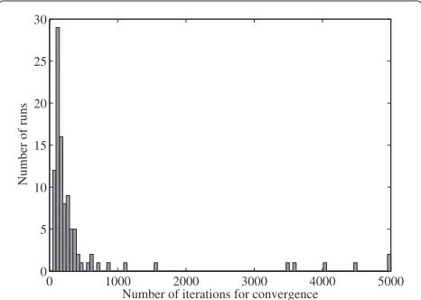
the spreading codes are unknown, the convergence speed is much slower. In this situation, we make use of eigen-analysis to initialize the ALS algorithm [20], and we have discarded 1% of the total number of runs for the BER calculation, corresponding to inevitable non-convergent runs, typical in ALS-type algorithms due to their sensi-tivity to initialization [40]. As an illustrative example, we have simulated a system withMt = Mr = 2,K =2,P =
8,N = 10,R = Q = 8 (i.e., R(q) = 1,q = 1,. . .,Q) and SNR = 30 dB. For this system configuration, Figure 3 depicts an histogram of the required number of iterations for convergence of the ALS algorithm. The histogram was based on 100 Monte Carlo runs. In this example, 92% of the runs have converged within the first 1,000 iterations.
6.1 Semi-blind ALS versus ZF receivers
The following simulation results illustrate the perfor-mance of the SFSM MIMO system using the ALS receiver described in Section 5.4. The main objectives are
1. To compare the performance of the semi-blind ALS receiver with that of the perfect ZF receiver; 2. To compare the SFSM MIMO system with other
CDMA–MIMO systems when ALS estimation is used;
0 1000 2000 3000 4000 5000
0 5 10 15 20 25 30
Number of runs
Number of iterations for convergence
Figure 3ALS algorithm: histogram of the number of iterations for convergence.
3 6 9 12 15 18 21
10−5 10−4 10−3 10−2 10−1 100
SNR (dB)
BER
M
t=2, Mr=2, K=2, R=8, Q=4, P=8, N=10
ALS (channel A) ZF (channel A) ALS (channel B) ZF (channel B)
Figure 4Comparison between semi-blind ALS and ZF receivers.
3. To evaluate the channel estimation accuracy as a function of the SNR.
All the simulations were performed assuming F = 64 subcarriers divided into groups of K = 2 or K = 4 subcarriers.
As a reference for comparison, in Figure 4, we compare the performance of the semi-blind ALS receiver with that of the ZF receiver described in Section 4, which assumes perfect channel and code knowledge. Our aim is to deter-mine the performance loss due to semi-blind receiver processing in the SFSM MIMO system. We assume Mt = Mr = 2,K = 2,P = 8,N = 10, Q = 4, and R(q) = 2,q = 1,. . ., 4. We can observe that the perfor-mance loss of the proposed receiver in comparison with the perfect ZF receiver is around 5 dB for channel A and 2 dB for channel B, for a BER equal to 10−3. In particu-lar, the slope of the BER curves is approximately the same, which means that the proposed receiver presents the same BER improvement as the ZF receiver as a function of the SNR. Also, both receivers perform better with channel B due to the increased multipath diversity.
6.2 Performance for different system loads
The next results illustrate the performance of the pro-posed receiver for different system loads. From now on, the ITU channel B is considered in all the simulations. We assumeMt = 2,K = 2,P = 16, andN = 20 while the
number of users is varied (Q = 4, 6, and 8). Each user transmits two data streams (R(q) = 2,q = 1,. . .,Q). We assumeMr = 1 or 2. Note that these configurations are
challenging in terms of receiver spatial diversity, sinceMr
condition (38) is satisfied in the chosen configurations. In fact, as can be observed from Figure 5, semi-blind recov-ery of symbol, channel, and codes is achieved even when Mr = 1. For instance, with Mr = 2 receive antennas,
increasing the number of users fromQ= 4 toQ= 6, or fromQ = 6 toQ = 8, implies nearly a 2-dB increase in the required SNR for a target BER of 10−2. We can also note that the BER performance is more sensitive to a vari-ation in the system load whenMr = 2 receive antennas
are used.
6.3 Comparison with the MCDS-CDMA system
The MCDS-CDMA system is a multicarrier extension of the classical DS-CDMA to frequency-selective chan-nels, by performing the spreading operation in the time-domain at each subcarrier [7]. As shown in Section 3.3, the PARAFAC modeling is also valid to model the MCDS-CDMA system, which is a special case of the proposed SFSM MIMO system, where space and frequency spread-ings are not used (i.e., Mt = 1 and K = 1). We now
compare the performance of both systems using the same PARAFAC-based ALS receiver with knowledge of the spreading codes. The perfect ZF receiver was also simu-lated for both systems as a reference for comparison. By comparing SFSM with MCDS-CDMA, we can verify the impact of space and frequency spreadings as a distinguish-ing feature of the SFSM MIMO system. Here, we assume Mr =2,P=8,N=50, andQ=8, each user transmitting
a single data stream (i.e.,R(q) = 1,q =1,. . ., 8). Figure 6 shows the substantial performance gain obtained with the proposed system, which corroborates the advantages of space and frequency spreadings. We can also note that the gap between ALS and ZF receivers is smaller when SFSM MIMO is used.
3 6 9 12 15 18 21
10−5 10−4 10−3 10−2 10−1 100
SNR (dB)
BER
Mt=2, K=2, P=16, N=20 Q=8 (Mr=1) Q=6 (Mr=1)
Q=4 (Mr=1) Q=8 (Mr=2)
Q=6 (Mr=2)
Q=4 (Mr=2)
Figure 5BER versus SNR with semi-blind ALS receiver(different system loads).
3 6 9 12 15 18 21
10−5 10−4 10−3 10−2 10−1 100
BER
Mr=2, R= Q=8, P=8, N=50
MCDS−CDMA+ALS (Mt =1, K=1) MCDS−CDMA + ZF (Mt =1, K=1) SFSM+ALS ( Mt =2, K=2) SFSM+ZF ( Mt =2, K=2)
SNR (dB)
Figure 6SFSM versus MCDS-CDMA (ALS versus ZF receivers).
6.4 Comparison with the SSSMA system
In [10], an MC-SSSMA system was proposed to provide space and frequency diversities in the forward link of a MIMO wireless system. The space–frequency spread-ing model proposed therein is a generalization of [45] to frequency-selective channels. The multicarrier SSSMA system has some similarity with the proposed SFSM MIMO system in the sense that space and frequency-domain spreadings are performed. In [10], a joint space– time spreading is used by means of Hadamard codes (its structure is detailed in [11]), while our approach uses separate space and frequency spreadings using Vander-monde codes. In Figure 7, the performances of SSSMA and SFSM MIMO are compared. We assume Mt = 2
transmit antennas,Mr = 1 or 2,F = 64 andK = 2. For
a fair comparison, we adjust the transmit parameters and
3 6 9 12 15 18 21
10−3 10−2 10−1 100
SNR (dB)
BER
M t=2, N=10
SSSMA, M
r=1 (known channel) SFSM, M
r=1 (semi−blind) SSSMA, M
r=2 (known channel) SFSM, M
r=2 (semi−blind)
3 6 9 12 15 18 21 24 27 30 10−2
10−1 100
SNR (dB)
RMSE
Mt=2, R=4, P=2, N=10 Mr=1 M
r=2
Figure 8RMSE of the estimated channel.
the modulation to keep the same data rate for both sys-tems. The SSSMA scheme assumesR = 8,P = 2, and BPSK. For the proposed SFSM scheme we haveR = 4, P = 4, and 16-QAM. In this case, both schemes have a rate of 2 bits per channel use. For the SSSMA system, a ZF receiver with perfect channel knowledge is used. For the proposed SFSM MIMO system, a semi-blind estimation without channel knowledge is used. The spreading codes are assumed to be known at the receiver for both systems. Note that for Mr = 1, SSSMA exhibits a poor
perfor-mance. This is due to the fact that multiuser detection in the SSSMA system requires Mr ≥ Mt. This
con-straint is not necessary in the SFSM MIMO system that makes an efficient use of the frequency diversity to sepa-rate the transmitted data streams when spatial diversity is not available at the receiver. ForMr = 2, SSSMA
outper-forms SFSM MIMO over the low-to-medium SNR range. For higher SNR values, the proposed system has superior performance. The slope of the BER curves indicates that the proposed SFSM scheme has a higher diversity gain.
6.5 Channel estimation performance
The channel estimation accuracy of the semi-blind ALS receiver is now evaluated from a root mean square error (RMSE) measure obtained from 100 Monte Carlo runs. The overall RMSE is calculated using the following formula:
RMSE=
! ! " 1
100MtMr 100
i=1
H¯(i)− ¯H 2
F,
where H¯(i) is the channel matrix estimated at the ith
Monte Carlo simulation. The following system configura-tion is considered for the SFSM MIMO system:Q = 1, Mt = 2,P = K = 2,R = 4,N = 10, andMr = 1
or 2. We can observe from Figure 8 that the RMSE has a linear decrease as a function of the SNR in both cases. UsingMr = 2 antennas provides a performance gain of
3 dB over the single receive antenna case. Such a gain obvi-ously comes from the increased receiver spatial diversity that helps the separation of the data streams, despite the larger number of parameters to estimate.
7 Conclusion
We have proposed a unified tensor model for MIMO communication systems with SFSM. The proposed model unifies several existing multiple-access/multiple-antenna communication systems. We have shown that the received signal can be formulated as a trilinear PARAFAC model, and capitalizing on its uniqueness property we have put in evidence lower bounds on the design parameters (num-ber of transmit/receive antennas, subcarriers, symbols per data stream, and spreading length) for a joint symbol-code-channel recovery. The obtained conditions help the understanding of the existing tradeoffs involving space, frequency, and code diversities that are inherent to the SFSM MIMO system. The performance of the proposed receiver using a semi-blind ALS algorithm has been illus-trated by means of computer simulations under realistic channel models and system parameters, and a comparison with other multiple-antenna CDMA-based systems has been made. Perspectives of this work include an investiga-tion of the impact of different transmit antenna, spreading code, and subcarrier allocation schemes on the design and performance of the proposed tensor-based receiver. We believe that these features could be integrated into the SFSM system by modeling the received signals using a CONFAC tensor model [18]. In this case, identifiability can be investigated using the recently established results on the partial uniqueness of constrained tensor decompo-sitions [46,47]. The impact of non-perfect users’ synchro-nization on the receiver performance is also a subject for a future work.
Endnotes
aFor notational convenience, we omit the noise terms
in the following developments. They will be added later, when the receiver algorithm is presented.
bThis means that any alternative triplet{ ˜G,S˜,C}˜
satisfy-ing model (19) is related to the true triplet{G,S,C}by the following equalities:G˜ =G1,S˜=S2,C˜ =C3,
whereis a permutation matrix andi,i = 1, 2, 3, are
diagonal (scaling) matrices such that123=IR. cThe Kruskal-rank ofAis equal toκif every subset ofκ
columns ofAis linearly independent.
dSee [20,40] for further details about the ALS algorithm.
Competing interests