Evaluating and optimizing the parameters
of an unsupervised graph-based WSD algorithm
Eneko Agirre, David Mart´ınez, Oier L´opez de Lacalle and Aitor Soroa
IXA NLP Group University of Basque Country
Donostia, Basque Contry [email protected]
Abstract
V´eronis (2004) has recently proposed an innovative unsupervised algorithm for word sense disambiguation based on small-world graphs called HyperLex. This paper explores two sides of the algorithm. First, we extend V´eronis’ work by opti-mizing the free parameters (on a set of words which is different to the target set). Second, given that the empirical compar-ison among unsupervised systems (and with respect to supervised systems) is sel-dom made, we used hand-tagged corpora to map the induced senses to a standard lexicon (WordNet) and a publicly avail-able gold standard (Senseval 3 English Lexical Sample). Our results for nouns show that thanks to the optimization of parameters and the mapping method, Hy-perLex obtains results close to supervised systems using the same kind of
bag-of-words features. Given the information
loss inherent in any mapping step and the fact that the parameters were tuned for an-other set of words, these are very interest-ing results.
1 Introduction
Word sense disambiguation (WSD) is a key en-abling technology. Supervised WSD techniques are the best performing in public evaluations, but need large amounts of tagging data. Existing hand-annotated corpora like SemCor (Miller et al., 1993), which is annotated with WordNet senses (Fellbaum,
1998) allow for a small improvement over the simple most frequent sense heuristic, as attested in the all-words track of the last Senseval competition (Sny-der and Palmer, 2004). In theory, larger amounts of training data (SemCor has approx. 500M words) would improve the performance of supervised WSD, but no current project exists to provide such an ex-pensive resource.
Supervised WSD is based on the “fixed-list of senses” paradigm, where the senses for a target word are a closed list coming from a dictionary or
lex-icon. Lexicographers and semanticists have long
warned about the problems of such an approach, where senses are listed separately as discrete enti-ties, and have argued in favor of more complex rep-resentations, where, for instance, senses are dense regions in a continuum (Cruse, 2000).
Unsupervised WSD has followed this line of thinking, and tries to induce word senses directly from the corpus. Typical unsupervised WSD sys-tems involve clustering techniques, which group
to-gether similar examples. Given a set of induced
clusters (which represent word uses or senses1),
each new occurrence of the target word will be com-pared to the clusters and the most similar cluster will be selected as its sense.
Most of the unsupervised WSD work has been based on the vector space model (Sch¨utze, 1998; Pantel and Lin, 2002; Purandare and Pedersen, 2004), where each example is represented by a
vec-tor of features (e.g. the words occurring in the
context). Recently, V´eronis (V´eronis, 2004) has
1Unsupervised WSD approaches prefer the term ’word uses’ to ’word senses’. In this paper we use them interchangeably to refer to both the induced clusters, and to the word senses from some reference lexicon.
proposed HyperLex, an application of graph mod-els to WSD based on the small-world properties
of cooccurrence graphs. Hand inspection of the
clusters (called hubs in this setting) by the author was very positive, with hubs capturing the main senses of the words. Besides, hand inspection of the disambiguated occurrences yielded precisions over 95% (compared to a most frequent baseline of 73%) which is an outstanding figure for WSD systems.
We noticed that HyperLex had some free param-eters and had not been evaluated against a public gold standard. Besides, we were struck by the few works where supervised and unsupervised systems were evaluated on the same test data. In this pa-per we use an automatic method to map the induced senses to WordNet using hand-tagged corpora, en-abling the automatic evaluation against available gold standards (Senseval 3 English Lexical Sam-ple S3LS (Mihalcea et al., 2004)) and the automatic optimization of the free parameters of the method. The use of hand-tagged corpora for tagging makes this algorithm a mixture of unsupervised and super-vised: the method to induce senses in completely unsupervised, but the mapping is supervised (albeit very straightforward).
This paper is structured as follows. We first
present the graph-based algorithm as proposed by V´eronis, reviewing briefly the features of small-world graphs. Section 3 presents our framework for mapping and evaluating the induced hubs. Section 4 introduces parameter optimization. Section 5 shows the experiment setting and results. Section 6 ana-lyzes the results and presents related work. Finally, we draw the conclusions and advance future work.
2 HyperLex
Before presenting the HyperLex algorithm itself, we briefly introduce small-world graphs.
2.1 Small world graphs
The small-world nature of a graph can be explained in terms of its clustering coefficient and
characteris-tic path length. The clustering coefficient of a graph
shows the extent to which nodes tend to form con-nected groups that have many edges connecting each other in the group, and few edges leading out of the group. On the other side, the characteristic path
length represents “closeness” in a graph. See (Watts and Strogatz, 1998) for further details on these char-acteristics.
Randomly built graphs exhibit low clustering co-efficients and are believed to represent something very close to the minimal possible average path
length, at least in expectation. Perfectly ordered
graphs, on the other side, show high clustering coef-ficients but also high average path length. According to Watts and Strogatz (1998), small-world graphs lie between these two extremes: they exhibit high clus-tering coefficients, but short average path lengths.
Barabasi and Albert (1999) use the term “scale-free” to graphs whose degree probability follow a
power-law2. Specifically, scale free graphs follow
the property that the probability P(k)that a vertex
in the graph interacts withkother vertices decays as
a power-law, following P(k) ∼ k−α. It turns out
that in this kind of graphs there exist nodes centrally located and highly connected, called hubs.
2.2 The HyperLex algorithm for WSD
The HyperLex algorithm builds a cooccurrence graph for all pairs of words cooccurring in the con-text of the target word. V´eronis shows that this kind of graph fulfills the properties of small world graphs, and thus possess highly connected components in the graph. The centers or prototypes of these com-ponents, called hubs, eventually identify the main word uses (senses) of the target word.
We will briefly introduce the algorithm here, check (V´eronis, 2004) for further details. For each word to be disambiguated, a text corpus is collected, consisting of the paragraphs where the word occurs. From this corpus, a cooccurrence graph for the tar-get word is built. Nodes in the graph correspond to
the words3in the text (except the target word itself).
Two words appearing in the same paragraph are said to cooccur, and are connected with edges. Each edge is assigned with a weight which measures the rela-tive frequency of the two words cooccurring.
Specif-ically, letwij be the weight of the edge4connecting
2
Although scale-free graphs are not necessarily small worlds, a lot of real world networks are both scale-free and small worlds.
3Following V´eronis, we only work on nouns for the time being.
nodesiandj, then
wij = 1−max[P(i|j), P(j |i)]
P(i|j) = freqij
freqj and P(j|i) = freqij
freqi
The weight of an edge measures how tightly con-nected the two words are. Words which always
oc-cur together receive a weight of 0. Words rarely
cooccurring receive weights close to1.
Once the cooccurrence graph is built, a simple it-erative algorithm is executed to obtain its hubs. At each step, the algorithm finds the vertex with
high-est relative frequency5 in the graph, and, if it meets
some criteria, it is selected as a hub. These criteria are determined by a set of heuristic parameters, that will be explained later in Section 4. After a vertex is selected to be a hub, its neighbors are no longer eli-gible as hub candidates. At any time, if the next ver-tex candidate has a relative frequency below a cer-tain threshold, the algorithm stops.
Once the hubs are selected, each of them is linked
to the target word with edges weighting 0, and the
Minimum Spanning Tree (MST) of the whole graph
is calculated and stored.
The MST is then used to perform word sense dis-ambiguation, in the following way. For every in-stance of the target word, the words surrounding it are examined and confronted with the MST. By con-struction of the MST, words in it are placed under exactly one hub. Each word in the context receives
a set of scoress, with one score per hub, where all
scores are0except the one corresponding to the hub
where it is placed. If the scores are organized in a
score vector, all values are 0, except, say, the i-th
component, which receives a score d(hi, v), which
is the distance between the hubhiand the node
rep-resenting the wordv. Thus,d(hi, v)assigns a score
of 1 to hubs and the score decreases as the nodes
move away from the hub in the tree.
For a given occurrence of the target word, the score vectors of all the words in the context are added, and the hub that receives the maximum score is chosen.
5In cooccurrence graphs, the relative frequency of a vertex and its degree are linearly related, and it is therefore possible to avoid the costly computation of the degree.
Base corpus
hyperLex_wsd hyperLex_wsd hyperLex
Evaluator Tagged
corpus
Test corpus Mapping
corpus
MST
matrix Mapping
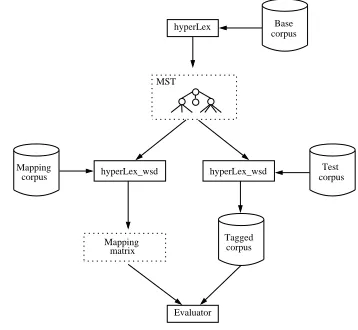
Figure 1: Design for the automatic mapping and evaluation
of HyperLex algorithm against a gold standard (test corpora).
3 Evaluating unsupervised WSD systems
All unsupervised WSD algorithms need some addi-tion in order to be evaluated. One alternative, as in (V´eronis, 2004), is to manually decide the correct-ness of the hubs assigned to each occurrence of the words. This approach has two main disadvantages. First, it is expensive to manually verify each occur-rence of the word, and different runs of the algo-rithm need to be evaluated in turn. Second, it is not an easy task to manually decide if an occurrence of a word effectively corresponds with the use of the word the assigned hub refers to, especially consid-ering that the person is given a short list of words linked to the hub. We also think that instead of judg-ing whether the hub returned by the algorithm is cor-rect, the person should have independently tagged the occurrence with hubs, which should have been then compared to the hub returned by the system.
A second alternative is to evaluate the system ac-cording to some performance in an application, e.g. information retrieval (Sch¨utze, 1998). This is a very attractive idea, but requires expensive system devel-opment and it is sometimes difficult to separate the reasons for the good (or bad) performance.
Ped-Default p180 p1800 p6700
value Range Best Range Best Range Best
p1 5 2-3 2 1-3 2 1-3 1
p2 10 3-4 3 2-4 3 2-4 3
p3 0.9 0.7-0.9 0.7 0.5-0.7 0.5 0.3-0.7 0.4
p4 4 4 4 4 4 4 4
p5 6 6-7 6 3-7 3 1-7 1
p6 0.8 0.5-0.8 0.6 0.4-0.8 0.7 0.6-0.95 0.95 p7 0.001 0.0005-0.001 0.0009 0.0005-0.001 0.0009 0.0009-0.003 0.001
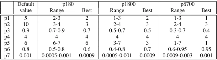
Table 1:Parameters of the HyperLex algorithm
ersen, 2004; Niu et al., 2005). See Section 6 for more details on these systems.
Yet another possibility is to evaluate the induced senses against a gold standard as a clustering task. Induced senses are clusters, gold standard senses are classes, and measures from the clustering literature like entropy or purity can be used. As we wanted to focus on the comparison against a standard data-set, we decided to leave aside this otherwise interesting option.
In this section we present a framework for au-tomatically evaluating unsupervised WSD systems against publicly available hand-tagged corpora. The framework uses three data sets, called Base corpus, Mapping corpus and Test corpus:
• The Base Corpus: a collection of examples of
the target word. The corpus is not annotated.
• The Mapping Corpus: a collection of examples
of the target word, where each corpus has been manually annotated with its sense.
• The Test Corpus: a separate collection, also
an-notated with senses.
The evaluation framework is depicted in Figure 1. The first step is to execute the HyperLex algorithm over the Base corpus in order to obtain the hubs of a target word, and the generated MST is stored. As stated before, the Base Corpus is not tagged, so the building of the MST is completely unsupervised.
In a second step (left part in Figure 1), we assign a hub score vector to each of the occurrences of target word in the Mapping corpus, using the MST calcu-lated in the previous step (following the WSD al-gorithm in Section 2.2). Using the hand-annotated sense information, we can compute a mapping
ma-trixM that relates hubs and senses in the following
way. Suppose there aremhubs andnsenses for the
target word. Then, M = {mij} 1 ≤i ≤ m,1 ≤
j ≤n, and eachmij =P(sj|hi), that is,mij is the
probability of a word having sensejgiven that it has
been assigned hub i. This probability can be
com-puted counting the times an occurrence with sense
sjhas been assigned hubhi.
This mapping matrix will be used to transform
any hub score vector ¯h = (h1, . . . , hm) returned
by the WSD algorithm into a sense score vector
¯
s = (s1, . . . , sn). It suffices to multiply the score
vector byM, i.e.,s¯= ¯hM.
In the last step (right part in Figure 1), we apply the WSD algorithm over the Test corpus, using again the MST generated in the first step, and returning a hub score vector for each occurrence of the target word in the test corpus. We then run the Evaluator,
which uses theM mapping matrix in order to
con-vert the hub score vector into a sense score vector. The Evaluator then compares the sense with high-est weight in the sense score vector to the sense that was manually assigned, and outputs the precision figures.
Preliminary experiments showed that, similar to other unsupervised systems, HyperLex performs better if it sees the test examples when building the graph. We therefore decided to include a copy of the training and test corpora in the base corpus (discard-ing all hand-tagged sense information, of course). Given the high efficiency of the algorithm this poses no practical problem (see efficiency figures in Sec-tion 6).
4 Tuning the parameters
As stated before, the behavior of the HyperLex algo-rithm is influenced by a set of heuristic parameters, that affect the way the cooccurrence graph is built, the number of induced hubs, and the way they are extracted from the graph. There are 7 parameters in total:
word train test MFS default p180 p1800 p6700 argument 221 111 51.4 51.4 51.4 51.4 51.4
arm 266 133 82.0 82.0 80.5 82.0 82.7
atmosphere 161 81 66.7 67.9 70.4 70.4 67.9 audience 200 100 67.0 69.0 71.0 74.0 77.0
bank 262 132 67.4 69.7 75.0 76.5 75.0
degree 256 128 60.9 60.9 60.9 62.5 63.3
difference 226 114 40.4 40.4 41.2 46.5 49.1
difficulty 46 23 17.4 30.4 30.4 39.1 26.1
disc 200 100 38.0 66.0 75.0 70.0 76.0
image 146 74 36.5 63.5 62.2 67.6 64.9
interest 185 93 41.9 49.5 41.9 47.3 51.6
judgment 62 32 28.1 28.1 28.1 53.1 50.0 organization 112 56 73.2 73.2 73.2 71.4 73.2
paper 232 117 25.6 42.7 39.3 47.9 53.8
party 230 116 62.1 67.2 64.7 65.5 67.2
performance 172 87 32.2 44.8 46.0 54.0 59.8
plan 166 84 82.1 81.0 79.8 81.0 83.3
shelter 196 98 44.9 45.9 49.0 48.0 54.1
sort 190 96 65.6 64.6 64.6 65.6 64.6
source 64 32 65.6 59.4 56.2 62.5 62.5
Average: 54.5 59.9 60.3 63.0 64.6
(Over S2LS) 51.9 56.2 57.5 58.7 60.0
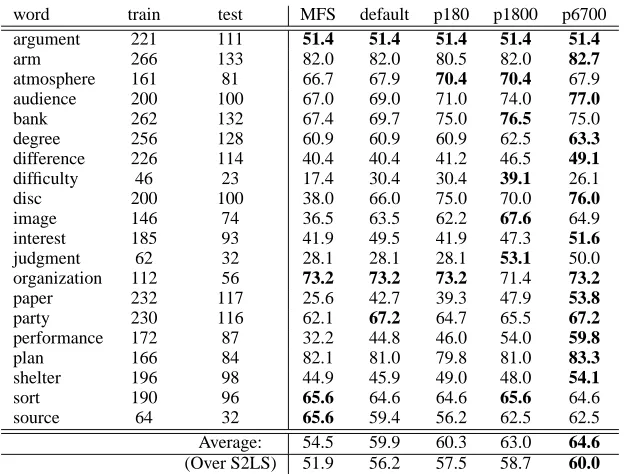
Table 2:Precision figures for nouns over the test corpus (S3LS). The second and third columns show the number of occurrences
in the train and test splits. The MFS column corresponds to the most frequent sense. The rest of columns correspond to different parameter settings: default for the default setting, p180 for the best combination over180, etc.. The last rows show the
micro-average over the S3LS run, and we also add the results on the S2LS dataset (different sets of nouns) to confirm that the same trends hold in both datasets.
p5 Minimum number of adjacent vertices a hub must have p6 Max. mean weight of the adjacent vertices of a hub p7 Minimum frequency of hubs
Table 1 lists the parameters of the HyperLex al-gorithm, and the default values proposed for them in the original work (second column).
Given that we have devised a method to efficiently evaluate the performance of HyperLex, we are able to tune the parameters against the gold standard. We first set a range for each of the parameters, and eval-uated the algorithm for each combination of the pa-rameters on a collection of examples of different words (Senseval 2 English lexical-sample, S2LS). This ensures that the chosen parameter set is valid for any noun, and is not overfitted to a small set of
nouns.6 The set of parameters that obtained the best
results in the S2LS run is then selected to be run against the S3LS dataset.
We first devised ranges for parameters amounting to 180 possible combinations (p180 column in Ta-ble 2), and then extended the ranges to amount to 1800 and 6700 combinations (columns p1800 and p6700).
6In fact, previous experiments showed that optimizing the parameters for each word did not yield better results.
5 Experiment setting and results
To evaluate the HyperLex algorithm in a standard
benchmark, we applied it to the20 nouns in S3LS.
We use the standard training-test split. Following the design in Section 3, we used both the training and test sets as the Base Corpus (ignoring the sense tags, of course). The Mapping Corpus comprised the training split only, and the Test corpus the test split only. The parameter tuning was done in a simi-lar fashion, but on the S2LS dataset.
In Table 2 we can see the number of examples of each word in the different corpus and the results of the algorithm. We indicate only precision, as the coverage is 100% in all cases. The left column, named MFS, shows the precision when always as-signing the most frequent sense (relative to the train split). This is the baseline of our algorithm as our algorithm does see the tags in the mapping step (see Section 6 for further comments on this issue).
The default column shows the results for the Hy-perLex algorithm with the default parameters as set by V´eronis, except for the minimum frequency of
the vertices (p2in Table 1), which according to some
preliminary experiments we set to3. As we can see,
0.55 0.56 0.57 0.58 0.59 0.6 0.61 0.62
0.5 0.55 0.6 0.65 0.7 0.75 0.8 0.85 0.9 0.95 1
Precision
Similarity Parameter space
Best fitting line
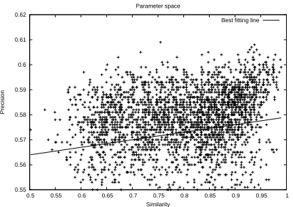
Figure 2: Dispersion plot of the parameter space for6700
combinations. The horizontal axis shows the similarity of a pa-rameter set w.r.t. the best papa-rameter set using the cosine. The vertical axis shows the precision in S2LS. The best fitting line is also depicted.
the MFS baseline by5.4points average, and in
al-most all words (except plan, sort and source).
The results for the best of180combinations of the
parameters improve the default setting (0.4overall),
Extending the parameter space to1800and6700
im-proves the precision up to63.0 and64.6, 10.1 over
the MFS (MFS only outperforms HyperLex in the best setting for two words). The same trend can be seen on the S2LS dataset, where the gain was more modest (note that the parameters were optimized for S2LS).
6 Discussion and related work
We first comment the results, doing some analysis, and then compare our results to those of V´eronis. Fi-nally we overview some relevant work and review the results of unsupervised systems on the S3LS benchmark.
6.1 Comments on the results
The results show clearly that our exploration of the parameter space was successful, with the widest pa-rameter space showing the best results.
In order to analyze whether the search in the pa-rameter space was making any sense, we drew a dis-persion plot (see Figure 2). In the top right-hand cor-ner we have the point corresponding to the best per-forming parameter set. If the parameters were not conditioning the good results, then we would have expected a random cloud of points. On the contrary, we can see that there is a clear tendency for those
default p180 p1800 p6700 hubs defined 9.2±3.8 15.3±5.7 38.6±11.8 77.7±18.7
used 8.4±3.5 14.4±5.3 30.4±9.3 45.2±13.3
senses defined 5.4±1.5 5.4±1.5 5.4±1.5 5.4±1.5
used 2.6±1.2 2.5±1 3.1±1.1 3.2±1.2
senses in test 5.1±1.3 - -
-Table 3: Average number of hubs and senses (along with the
standard deviation) for three parameter settings. Defined means the number of hubs induced, and used means the ones actually returned by HyperLex when disambiguating the test set. The same applies for senses, that is, defined means total number of senses (equal for all columns), and used means the senses that were actually used by HyperLex in the test set. The last row shows the actual number of senses used by the hand-annotators in the test set.
parameter sets most similar to the best one to obtain better results, and in fact the best fitting line shows a clearly ascending slope.
Regarding efficiency, our implementation of
Hy-perLex is extremely fast. Doing the1800
combina-tions takes 2 hours in a 2 AMD Opteron processors at 2GHz and 3Gb RAM. A single run (building the MST, mapping and tagging the test sentences) takes only 16 sec. For this reason, even if an on-line ver-sion would be in principle desirable, we think that this batch version is readily usable.
6.2 Comparison to (V´eronis, 2004)
Compared to V´eronis we are inducing larger num-bers of hubs (with different parameters), using less examples to build the graphs and obtaining more modest results (far from the 90’s). Regarding the lat-ter, our results are in the range of other S3LS WSD systems (see below), and the discrepancy can be ex-plained by the way V´eronis performed his evaluation (see Section 3).
Table 3 shows the average number of hubs for the four parameter settings. The average number of hubs for the default setting is larger than that of V´eronis (which ranges between 4 and 9 per word), but quite close to the average number of senses. The exploration of the parameter space prefers parame-ter settings with even larger number of hubs, and the figures shows that most of them are actually used for disambiguation. The table also shows that, after the mapping, less than half of the senses are actu-ally used, which seems to indicate that the mapping tends to favor the most frequent senses.
Regarding the actual values of the parameters
of some parameters (e.g. the minimum frequency of vertices) due to the smaller number of of exam-ples (V´eronis used from 1900 to 8700 examexam-ples per word). In theory, we could explore larger parame-ter spaces, but Table 1 shoes that the best setting for the 6700 combinations has no parameter in a range boundary (except p5, which cannot be further re-duced).
All in all, the best results are attained with smaller and more numerous hubs, a kind of micro-senses. A possible explanation for this discrepancy with V´eronis could be that he was inspecting by hand the hubs that he got, and perhaps was biased by the fact that he wanted the hubs to look more like stan-dard senses. At first we were uncomfortable with this behavior, so we checked whether HyperLex was degenerating into a trivial solution. We simulated a clustering algorithm returning one hub per
exam-ple, and its precision was40.1, well below the MFS
baseline. We also realized that our results are in accordance with some theories of word meaning, e.g. the “indefinitely large set of prototypes-within-prototypes” envisioned in (Cruse, 2000). We now think that the idea of having many micro-senses is very attractive for further exploration, especially if we are able to organize them into coarser hubs.
6.3 Comparison to related work
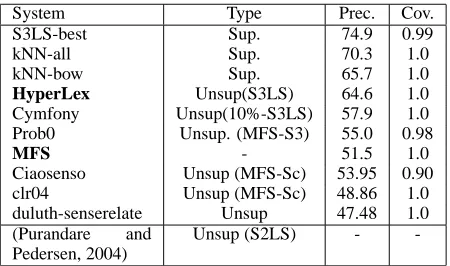
Table 4 shows the performance of different systems on the nouns of the S3LS benchmark. When not re-ported separately, we obtained the results for nouns running the official scorer program on the filtered results, as available in the S3LS web page. The sec-ond column shows the type of system (supervised, unsupervised).
We include three supervised systems, the winner of S3LS (Mihalcea et al., 2004), an in-house system (kNN-all, CITATION OMITTED) which uses opti-mized kNN, and the same in-house system restricted to bag-of-words features only (kNN-bow), i.e. dis-carding other local features like bigrams or trigrams (which is what most unsupervised systems do). The table shows that we are one point from the bag-of-words classifier kNN-bow, which is an impressive result if we take into account the information loss of the mapping step and that we tuned our parameters on a different set of words. The full kNN system is state-of-the-art, only 4 points below the S3LS
win-System Type Prec. Cov.
S3LS-best Sup. 74.9 0.99
kNN-all Sup. 70.3 1.0
kNN-bow Sup. 65.7 1.0
HyperLex Unsup(S3LS) 64.6 1.0
Cymfony Unsup(10%-S3LS) 57.9 1.0 Prob0 Unsup. (MFS-S3) 55.0 0.98
MFS - 51.5 1.0
Ciaosenso Unsup (MFS-Sc) 53.95 0.90 clr04 Unsup (MFS-Sc) 48.86 1.0 duluth-senserelate Unsup 47.48 1.0 (Purandare and
Pedersen, 2004)
Unsup (S2LS) -
-Table 4:Comparison of HyperLex and MFS baseline to S3LS
systems for nouns. The last system was evaluated on S2LS.
ner.
Table 4 also shows several unsupervised systems, all of which except Cymfony and (Purandare and Pedersen, 2004) participated in S3LS (check (Mi-halcea et al., 2004) for further details on the sys-tems). We classify them according to the amount of “supervision” they have: some have have access to most-frequent information (MFS-S3 if counted over S3LS, MFS-Sc if counted over SemCor), some use 10% of the S3LS training part for mapping (10%-S3LS), and some use the full amount of S3LS train-ing for mapptrain-ing (S3LS). Only one system (Duluth) did not use in any way hand-tagged corpora.
Given the different typology of unsupervised sys-tems, it’s unfair to draw definitive conclusions from a raw comparison of results. The system coming closer to ours is that described in (Niu et al., 2005). They use hand tagged corpora which does not need to include the target word to tune the parameters of a rather complex clustering method which does use local information (an exception to the rule of unsu-pervised systems). They do use the S3LS training corpus for mapping. For every sense the target word, three of its contexts in the train corpus are gathered (around 10% of the training data) and tagged. Each cluster is then related with its most frequent sense. Only one cluster may be related to a specific sense, so if two or more clusters map to the same sense, only the largest of them is retained. The mapping method is similar to ours, but we use all the avail-able training data and allow for different hubs to be assigned to the same sense.
order bag-of-word context features to represent each instance of the corpus. They apply several clustering algorithms based on the vector space model, limiting the number of clusters to 7. They also use all avail-able training data for mapping, but given their small number of clusters they opt for a one-to-one map-ping which maximizes the assignment and discards the less frequent clusters. They also discard some difficult cases, like senses and words with low fre-quencies (10% of total occurrences and 90, respec-tively). The different test set and mapping system make the comparison difficult, but the fact that the best of their combinations beats MFS by 1 point on average (47.6% vs. 46.4%) for the selected nouns and senses make us think that our results are more robust (nearly 10% over MFS).
7 Conclusions and further work
This paper has explored two sides of HyperLex: the optimization of the free parameters, and the empir-ical comparison on a standard benchmark against other WSD systems. We use hand-tagged corpora to map the induced senses to WordNet senses.
Regarding the optimization of parameters, we used a another testbed (S2LS) comprising different words to select the best parameter. We consistently improve the results of the parameters by V´eronis, which is not perhaps so surprising, but the method allows to fine-tune the parameters automatically to a given corpus given a small test set.
Comparing unsupervised systems against super-vised systems is seldom done. Our results indicate that HyperLex with the supervised mapping is on par with a state-of-the-art system which uses bag-of-words features only. Given the information loss inherent to any mapping, this is an impressive re-sult. The comparison to other unsupervised systems is difficult, as each one uses a different mapping strategy and a different amount of supervision.
For the future, we would like to look more closely the micro-senses induced by HyperLex, and see if we can group them into coarser clusters. We also plan to apply the parameters to the Senseval 3 all-words task, which seems well fit for HyperLex: the best supervised system only outperforms MFS by a few points in this setting, and the training cor-pora used (Semcor) is not related to the test corcor-pora
(mainly Wall Street Journal texts).
Graph models have been very successful in some settings (e.g. the PageRank algorithm of Google), and have been rediscovered recently for natural lan-guage tasks like knowledge-based WSD, textual en-tailment, summarization and dependency parsing. We would like to test other such algorithms in the same conditions, and explore their potential to inte-grate different kinds of information, especially the local or syntactic features so successfully used by supervised systems, but also more heterogeneous in-formation from knowledge bases.
References
A. L. Barabasi and R. Albert. 1999. Emergence of scal-ing in random networks. Science, 286(5439):509–512, October.
D. A. Cruse, 2000. Polysemy: Theoretical and Com-putational Approaches, chapter Aspects of the Micro-structure of Word Meanings. OUP.
C. Fellbaum. 1998. WordNet: An Electronic Lexical Database. MIT Press.
R. Mihalcea, T. Chklovski, and A. Kilgarriff. 2004. The senseval-3 english lexical sample task. In R. Mihal-cea and P. Edmonds, editors, Senseval-3 proceedings, pages 25–28. ACL, July.
G.A. Miller, C. Leacock, R. Tengi, and R.Bunker. 1993. A semantic concordance. In Proc. of the ARPA HLT workshop.
C. Niu, W. Li, R. K. Srihari, and H. Li. 2005. Word independent context pair classification model for word sense disambiguation. In Proc. of CoNLL-2005. P. Pantel and D. Lin. 2002. Discovering word senses
from text. In Proc. of KDD02.
A. Purandare and T. Pedersen. 2004. Word sense dis-crimination by clustering contexts in vector and simi-larity spaces. In Proc. of CoNLL-2004.
H. Sch ¨utze. 1998. Automatic word sense discrimination. Computational Linguistics, 24(1):97–123.
B. Snyder and M. Palmer. 2004. The english all-words task. In Proc. of SENSEVAL.
J. V´eronis. 2004. HyperLex: lexical cartography for in-formation retrieval. Computer Speech & Language, 18(3):223–252.