R E S E A R C H
Open Access
Denumerably many positive solutions for
a
n
-dimensional higher-order singular
fractional differential system
Ping Li and Meiqiang Feng
**Correspondence: [email protected] School of Applied Science, Beijing Information Science & Technology University, Beijing, People’s Republic of China
Abstract
This paper investigates the existence of denumerably many positive solutions and two infinite families of positive solutions for then-dimensional higher-order fractional differential systemDα
0+x(t) +
λ
g(t)f(t,x(t)) = 0, 0 <t< 1. The vector-valued functionxis defined byx= [x1,x2,. . .,xn],g(t) = diag[g1(t),g2(t),. . .,gn(t)], wheregi∈Lp[0, 1] for somep≥1,i= 1, 2,. . .,n, and has infinitely many singularities in [0,12). Our methods employ the fixed point theorems combined with the partially ordered structure of a Banach space.Keywords: Denumerably many positive solutions;n-dimensional higher-order fractional differential system; Infinitely many singularities; Matrix theory; Fixed point theorems in cones
1 Introduction
Fractional differential equations, which provide a natural description of memory and hereditary properties of various materials and processes, are regarded as an important mathematical tool for better understanding of many real world problems in applied sci-ences, such as physics, chemistry, aerodynamics, Bode’s analysis of feedback amplifiers, capacitor theory, electrical circuits and so on. This is the main advantage of fractional differential equations in comparison with classical integer-order models. For applications and explanations of fractional differential equations, we refer the reader to the texts [1–4]. In particular, many authors have shown great interest in the subject of fractional-order boundary value problems (BVPs), and many excellent results for BVPs equipped with dif-ferent kinds of boundary conditions have been obtained, for more details and examples, see [5–23] and the references cited therein.
Moreover, Alsulami, Ntouyas, Agarwal, Ahmad and Alsaedi [24] pointed out that frac-tional differential system constitute an important and interesting field of investigation because of their applications in many real world problems such as anomalous diffu-sion [25], disease models [26–28], ecological models [29], synchronization of chaotic systems [30–32] and so forth. For some theoretical work on the fractional differential system, we refer the reader to [33–41]. However, it is not difficult to see that there are only a few results onn-dimensional fractional differential systems; for example, see
[42, 43], especially for n-dimensional higher-order singular fractional differential sys-tems.
At the same time, we notice that a class of boundary value problem with integral bound-ary conditions have attracted the attention of Boucherif [44], Zhang et al. [45, 46], Hao et al. [47], Jiang et al. [48, 49], Kong [50], Feng et al. [51], Ahmad et al. [52], Mao et al. [53], and Liu et al. [54, 55].
To the best of our knowledge, in the literature there are not articles on denumer-ably many positive solutions for the analogous ofn-dimensional higher-order singular fractional differential with integral boundary conditions. More precisely, the study of
gi∈Lp[0, 1] for somep≥1,i= 1, 2, . . . ,n, and having infinitely many singularities in [0,12),
is still open for the followingn-dimensional higher-order singular fractional differential system:
Dα0+x(t) +λg(t)f
t, x(t)= 0, 0 <t< 1 (1.1)
with the following boundary conditions:
⎧ ⎨ ⎩
x(0) = x(0) =· · ·= x(n–2)(0) = 0,
ax(1) +bx(1) =01h(t)x(t)dt,
(1.2)
where Dα
0+is the standard Riemann–Liouville fractional derivative of ordern– 1 <α≤n,
n≥3,λis a positive parameter,a> 0,b≥0 anda> (α– 1)b. In addition,
x= [x1,x2, . . . ,xn],
g(t) =diagg1(t),g2(t), . . . ,gn(t) ,
f(t, x) =f1(t, x),f2(t, x), . . . ,fi(t, x), . . . ,fn(t, x)
,
h(t) =diagh1(t),h2(t), . . . ,hn(t) ,
where
fi(t, x) =fi(t,x1,x2, . . . ,xi, . . . ,xn).
Therefore, system (1.1) means that
⎧ ⎪ ⎪ ⎪ ⎪ ⎪ ⎨ ⎪ ⎪ ⎪ ⎪ ⎪ ⎩
–Dα
0+x1(t) =λg1(t)f1(t,x1(t),x2(t), . . . ,xn(t)), 0 <t< 1,
–Dα
0+x2(t) =λg2(t)f2(t,x1(t),x2(t), . . . ,xn(t)), 0 <t< 1,
· · · ·,
–Dα0+xn(t) =λgn(t)fn(t,x1(t),x2(t), . . . ,xn(t)), 0 <t< 1,
(1.2) means that ⎧
⎪ ⎪ ⎪ ⎪ ⎪ ⎪ ⎪ ⎪ ⎪ ⎪ ⎪ ⎪ ⎪ ⎪ ⎨ ⎪ ⎪ ⎪ ⎪ ⎪ ⎪ ⎪ ⎪ ⎪ ⎪ ⎪ ⎪ ⎪ ⎪ ⎩
x1(0) =x1(1) =· · ·=x(1n–2)(t) = 0,
ax1(1) +bx1(1) =
1
0 h1(t)x1(t)dt,
x2(0) =x2(1) =· · ·=x(2n–2)(t) = 0,
ax2(1) +bx2(1) =
1
0 h2(t)x2(t)dt,
· · ·,
xn(0) =xn(1) =· · ·=x(nn–2)(t) = 0,
axn(1) +bxn(1) =
1
0 hn(t)xn(t)dt.
(1.4)
Here we emphasize that our problem is new in the sense of then-dimensional higher-order singular fractional differential systems introduced here. To the best of our knowl-edge, the existence of single or multiple positive solutions forn-dimensional higher-order singular fractional differential system (1.1)–(1.2) has not yet to be studied, especially for the existence of denumerably many positive solutions and two infinite families of positive solutions for system (1.1)–(1.2). In consequence, our main results of the present work will be a useful contribution to the existing literature on the topic ofn-dimensional higher-order singular fractional differential systems. The existence of denumerably many posi-tive solutions and two infinite families of posiposi-tive solutions for the given problem are new, though they are proved by applying the well-known method based on the fixed theory in cones and the partially ordered structure of Banach space.
Throughout this paper, we usei= 1, 2, . . . ,n, unless otherwise stated. Let the components of g and f satisfy the following conditions:
(H1) gi∈Lp[0, 1]for somep∈[1, +∞), and there existsNi> 0such thatgi(t)≥Nia.e. on J= [0, 1];
(H2) there exists a sequence{tj}∞j=1such thatt1<12,tj↓t0> 0andlimt→tjgi(t) = +∞for
allj= 1, 2, . . .;
(H3) fi(t, x)∈C(J×R+n,R+), whereR+= [0, +∞)andRn+=
n
i=1R+;
(H4) hi∈L1[0, 1]is nonnegative withμi∈[0,a– (α– 1)b), whereμiis defined in (2.18).
The plan of this paper is as follows. We shall introduce some basic definitions and lem-mas of fractional calculus in the rest of this section. In Sect. 2, we give the expression and new properties of Green’s function associated with system (1.1)–(1.2). In Sect. 3, we present some characteristics of the integral operator associated with system (1.1)–(1.2) and state two fixed point theorems in cones. In Sect. 4, we discuss the existence of denu-merably many positive solutions of system (1.1)–(1.2). In Sect. 5, we will prove the exis-tence of two infinite families of positive solutions of system (1.1)–(1.2). In Sect. 6, we give some interesting comments and remarks associated with system (1.1)–(1.2).
In the rest of this section, we introduce some basic definitions and lemmas of fractional calculus.
Definition 1.1([2]) The integral
Iα
0+f(x) =
1
(α) x
0
f(t)
(x–t)1–αdt, x> 0,
Definition 1.2([2]) For a functionf(x) given in the interval [0, 1), the expression
Dα0+f(x) = 1
(n–α)
d dx
n x
0
f(t) (x–t)α–n+1dt,
wheren= [α]+1, [α] denotes the integer part of numberα, is called the Riemann–Liouville fractional derivative of orderα.
Lemma 1.1([7]) Assume that u∈C(0, 1)∩L(0, 1)with a fractional derivative of order α> 0that belongs to u∈C(0, 1)∩L(0, 1).Then
I0+αDα0+u(t) =u(t) +C1tα–1+C2tα–2+· · ·+ +CNtα–N,
for some Ci∈R,i= 1, 2, . . . ,N,where N is the smallest integer greater than or equal toα.
2 Green’s function associated with system (1.1)–(1.2)
In this section, we discuss the expression and properties of the Green’s function associated with system (1.1)–(1.2).
Let y = [y1,y2, . . . ,yn]. Consider the fractional differential system
Dα0+x(t) + y(t) = 0, 0 <t< 1, (2.1)
with the boundary conditions (1.2). Equation (2.1) means that
⎧ ⎪ ⎪ ⎪ ⎪ ⎪ ⎨ ⎪ ⎪ ⎪ ⎪ ⎪ ⎩
–Dα
0+x1(t) =y1(t), 0 <t< 1,
–Dα
0+x2(t) =y2(t), 0 <t< 1,
· · · ·, –Dα
0+xn(t) =yn(t), 0 <t< 1.
(2.2)
Lemma 2.1 If01hi(t)tα–1dt=a– (α– 1)b and yi∈C[0, 1],i= 1, 2, . . . ,n,then system(2.1)–
(1.2)has a unique solutionx= [x1,x2, . . . ,xn]∈Rn+in which xi(t)is given by
xi(t) =
1
0
Gi(t,s)yi(s)ds, (2.3)
where
Gi(t,s) =G1(t,s) +G2i(t,s), (2.4)
G1(t,s) =
1
(α)(a+ (α– 1)b) ⎧ ⎪ ⎪ ⎪ ⎪ ⎪ ⎨ ⎪ ⎪ ⎪ ⎪ ⎪ ⎩
atα–1(1 –s)α–1+b(α– 1)tα–1(1 –s)α–2
– (a+ (α– 1)b)(t–s)α–1, 0≤s≤t≤1,
atα–1(1 –s)α–1+b(α– 1)tα–1(1 –s)α–2,
0≤t≤s≤1,
(2.5)
G2i(t,s) =
tα–1
(a– (α– 1)b) –01hi(t)tα–1dt
1
0
Proof By the fact that system (2.1)–(1.2) is equivalent to system (2.2)–(1.4). Therefore system (2.1)–(1.2) has a unique solution x which is equivalent to the following sys-tem:
⎧ ⎪ ⎪ ⎨ ⎪ ⎪ ⎩
Dα
0+xi(t) +yi(t) = 0, 0 <t< 1, xi(0) =xi(0) =· · ·=x
(n–2)
i (0) = 0, axi(1) +bxi(1) =
1
0 hi(t)xi(t)dt
(2.7)
has a unique solutionxi, which is given by (2.3).
Next, by a proof which is similar to that of Lemma 2.1 in [8], we can show that (2.3)
holds. This finishes the proof of Lemma 2.1.
From (2.4), (2.5) and (2.6), we can prove thatGi(t,s),G1(t,s) andG2i(t,s) have the
fol-lowing properties.
Proposition 2.1 The function G1(t,s)defined by(2.5)satisfies
(i) G1(t,s)≥0is continuous for allt,s∈J,G1(t,s) > 0,∀t,s∈(0, 1);
(ii) For allt∈J,s∈(0, 1),we have
G1(t,s)≤G1
τ(s),s
=aτ(s)α–1(1 –s)α–1+b(α– 1)τ(s)α–1
(1 –s)α–2
–a+b(α– 1)τ(s) –sα–1/(α)a+b(α– 1), (2.8)
where
τ(s) = s 1 –e(s)(1 –s)αα–1–2
, e(s) =
a+b(α–1) 1–s a+b(α– 1)
1
α–2
. (2.9)
Proof (i) It is obvious thatG1(t,s) is continuous onJ×JandG1(t,s)≥0 whens≥t.
For 0≤s<t≤1, we have
atα–1(1 –s)α–1+b(α– 1)tα–1(1 –s)α–2–a+ (α– 1)b(t–s)α–1
= (1 –s)α–1a+b(α– 1)(1 –s)–1tα–1–a+b(α– 1)t–s 1 –s
α–1
≥0.
So, by (2.5), we have
G1(t,s)≥0, ∀t,s∈J.
(ii) Sincen– 1 <α≤n,n≥3, it is clear thatG1(t,s) is increasing with respect totfor
0≤t≤s≤1.
On the other hand, from the definition ofG1(t,s), for givens∈(0, 1),s<t≤1, we have
∂G1(t,s)
∂t =
α– 1
(α)(a+b(α– 1))
atα–2(1 –s)α–1+b(α– 1)tα–2(1 –s)α–2
–a+b(α– 1) (t–s)α–2.
Let
∂G1(t,s)
∂t = 0.
Then we have
atα–2(1 –s)α–1+b(α– 1)tα–2(1 –s)α–2=a+b(α– 1) (t–s)α–2,
and so
a+b(α– 1) 1 –s
(1 –s)α–1=a+b(α– 1) 1 –s
t
α–2
. (2.10)
Noticingα> 2, from (2.10), we have
t= s
1 –e(s)(1 –s)αα–1–2
=:τ(s), e(s) =
a+b(1–α–1)s
a+b(α– 1) 1
α–2
.
Then, for givens∈(0, 1), we haveG1(t,s) arriving at a maximum at (τ(s),s) whens<t.
From this, together with the fact that G1(t,s) is increasing on s≥t, we see that (2.8)
holds.
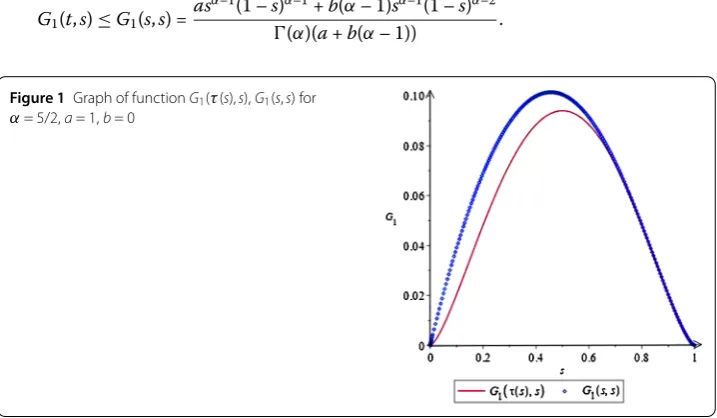
Remark2.1 From Fig. 1, we can seeG1(s,s)≤G1(τ(s),s) forα> 2. If 1 <α≤2, then
G1(t,s)≤G1(s,s) =
asα–1(1 –s)α–1+b(α– 1)sα–1(1 –s)α–2
(α)(a+b(α– 1)) .
Figure 1Graph of functionG1(τ(s),s),G1(s,s) for
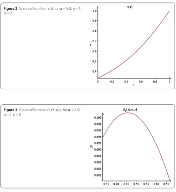
Figure 2Graph of functionτ(s), forα= 5/2,a= 1,
b= 0
Figure 3Graph of functionG1(τ(s),s), forα= 5/2,
a= 1,b= 0
Remark2.2 From Fig. 2, we can see thatτ(s) is increasing with respect tos.
Remark2.3 From Fig. 3, we can see thatG1(τ(s),s) > 0 fors∈Jθ = [θ, 1 –θ], whereθ ∈ (0,12).
Remark2.4 LetG¯1(τ(s),s) =a(τ(s))α–1(1 –s)α–1+b(α– 1)(τ(s))α–1(1 –s)α–2– (a+b(α–
1))(τ(s) –s)α–1. From (2.8), fors∈(0, 1), we have
dG¯1(τ(s),s)
ds = –a(α– 1)(1 –s)
α–2τ(s)α–1
+a(α– 1)(1 –s)α–1τ(s)α–1τ(s)
–b(α– 1)(α– 2)(1 –s)α–3τ(s)α–1
+b(α– 1)2(1 –s)α–2τ(s)α–2τ(s)
Remark2.5 From (2.11), we have
lim
s→0
dG¯1(τ(s),s)
ds = (α– 1)
–a+b(α– 2)α– 2
α– 1 α–1
+a+b(α– 1)α– 2
α– 1 α–2
=
α– 2
α– 1 α–2
a+b(2α– 3)
:=f(α).
Remark2.6 Noticing thatα> 2, it follows from Remark 2.5 thatf(α) > 0.
Remark2.7 It is interesting to point out thatf(α) is not decreasing with respect toαin the case witha> 0 andb> 0. Ifa> 0 andb= 0, thenf(α) is decreasing with respect toα.
Proposition 2.2 There existsγ > 0such that
min
t∈[θ,1–θ]G1(t,s)≥γG1
τ(s),s, ∀s∈J. (2.12)
Proof Fort∈Jθ, we divide the proof into the following three cases fors∈J.
Case 1.Ifs∈Jθ, then from (i) of Proposition 2.1 and Remark 2.3, we have
G1(t,s) > 0, G1
τ(s),s> 0, ∀t,s∈Jθ.
It is obvious thatG1(t,s) andG1(τ(s),s) are bounded onJθ. So, there exists a constantγ1> 0
such that
G1(t,s)≥γ1G1
τ(s),s, ∀t,s∈Jθ. (2.13)
Case 2.Ifs∈[1 –θ, 1], then from (2.5), we have
G1(t,s) =
atα–1(1 –s)α–1+b(α– 1)tα–1(1 –s)α–2
(α)(a+b(α– 1)) .
On the other hand, from the definition ofτ(s), we see thatτ(s) takes its maximum 1 at
s= 1. So
G1
τ(s),s=aτ(s)α–1(1 –s)α–1+b(α– 1)τ(s)α–1(1 –s)α–2
–a+b(α– 1)τ(s) –sα–1/(α)a+b(α– 1)
≤a(τ(s))α–1(1 –s)α–1+b(α– 1)(τ(s))α–1(1 –s)α–2 (α)(a+b(α– 1))
=(τ(s)) α–1
tα–1
a(1 –s)α–1tα–1+b(α– 1)(1 –s)α–2tα–1
(α)(a+b(α– 1))
≤ 1
θα–1G1(t,s). (2.14)
Therefore,G1(t,s)≥θα–1G1(τ(s),s). Lettingθα–1=γ2, we have
G1(t,s)≥γ2G1
Case 3.Ifs∈[0,θ], from (i) of Proposition 2.1, it is clear that
G1(t,s) > 0, G1
τ(s),s> 0, ∀t∈Jθ,s∈(0,θ].
In view of the Remarks 2.4–2.6, we have
lim
s→0
G1(t,s)
G1(τ(s),s)
=lim
s→0
atα–1(1 –s)α–1+b(α– 1)tα–1(1 –s)α–2– (a+b(α– 1))(t–s)α–1
a(τ(s))α–1(1 –s)α–1+b(α– 1)(τ(s))α–1(1 –s)α–2– (a+b(α– 1))(τ(s) –s)α–1
=lim
s→0
–a(α– 1)tα–1(1 –s)α–2–b(α– 1)tα–1(1 –s)α–3
+ (α– 1)a+b(α– 1)(t–s)α–2dG¯1(τ(s),s)
ds
> 0. (2.16)
From (2.16), there exists a constantγ3such that
G1(t,s)≥γ3G1
τ(s),s. (2.17)
Lettingγ =min{γ1,γ2,γ3}and using (2.13), (2.15) and (2.17), it follows that (2.12) holds.
This completes the proof.
Let
μi=
1
0
hi(t)tα–1dt. (2.18)
Proposition 2.3 Ifμi∈[0,a–b(α– 1)),then we have
(i) G2i(t,s)≥0is continuous for allt,s∈J,G2i(t,s) > 0,∀t,s∈(0, 1);
(ii) G2i(t,s)≤(a–b(α1–1))–μi
1
0 hi(t)G1(t,s)dt,∀t∈J,s∈(0, 1).
Proof Using the properties ofG1(t,s), definition ofG2i(t,s), it can easily be shown that (i)
and (ii) hold.
Theorem 2.1 Ifμi∈[0,a–b(α– 1)),the function Gi(t,s)defined by(2.4)satisfies
(i) Gi(t,s)≥0is continuous for allt,s∈J,Gi(t,s) > 0,∀t,s∈(0, 1);
(ii) Gi(t,s)≤Gi(s)for eacht,s∈J,and
min
t∈[θ,1–θ]Gi(t,s)≥γ
∗G
i(s), ∀s∈J, (2.19)
where
γ∗=minγ,θα–1, Gi(s) =G1
τ(s),s+G2i(1,s), (2.20)
Proof (i) From Proposition 2.1 and Proposition 2.3, we see thatGi(t,s)≥0 is continuous
for allt,s∈J, andGi(t,s) > 0,∀t,s∈(0, 1).
(ii) From (ii) of Proposition 2.1 and (ii) of Proposition 2.3, we haveGi(t,s)≤Gi(s) for
eacht,s∈J.
Now, we show that (2.19) holds. In fact, from Proposition 2.2, we have
min t∈Jθ
Gi(t,s)≥γG1
τ(s),s+ θ α–1
(a–b(α– 1)) –μi
1
0
hi(t)G1(t,s)dt
≥γ∗
G1
τ(s),s+ 1 (a–b(α– 1)) –μi
1
0
hi(t)G1(t,s)dt
=γ∗Gi(s), ∀s∈J.
Then the proof of Theorem 2.1 is completed.
Remark2.8 From the definition ofγ∗, it is clear that 0 <γ∗< 1.
3 Preliminaries
LetE=C[0, 1], X =E× · · · × E n
, and, for any x = [x1,x2, . . . ,xn]∈X,
X=
n
i=1
sup t∈J
xi(t). (3.1)
Then (X,·) is a real Banach space.
To establish the existence of positive solutions to system (1.1)–(1.2), for a fixedθ∈(t0,12), we construct the cone Kθin X by
Kθ=
x= (x1,x2, . . . ,xn)∈X:xi(t)≥0,i= 1, 2, . . . ,n,t∈J,
min t∈[θ,1–θ]
n
i=1
xi(t)≥γ∗x
, (3.2)
whereγ∗is defined in (2.20), and it is easy to see Kθis a closed convex cone of X. Let{θj}∞j=1be such thattj+1<θj<tj,j= 1, 2, . . . . So we get 0 <· · ·<tj+1<θj<tj<· · ·<t3<
θ2<t2<θ1<t1<12< 1. Then, for anyj∈N, we define the cone Kθjby
Kθj=
x∈X:xi(t)≥0,t∈J,i= 1, 2, . . . ,n, min t∈[θj,1–θj]
n
i=1
xi(t)≥γj∗x
, (3.3)
where
γj∗=minγj,θjα–1
, (3.4)
hereγj=min{γ1j,γ2j,γ3j},γ1,γ2andγ3is similarly defined in (2.13), (2.14) and (2.17),
Also, for a positive numberτ, define Kτ θjby
Kτ θj=
x∈Kθj:x<τ
.
Let Tλ: Kθj→Xbe a map with components (T
1
λ,Tλ2, . . . ,Tλi, . . . ,Tλn). We understand that Tλx= (Tλ1x,Tλ2x, . . . ,Tλix, . . . ,Tλnx), where
Tλix
(t) =λ
1
0
Gi(t,s)gi(s)fi
s, x(s)ds, i= 1, 2, . . . ,n. (3.5)
Remark3.1 It follows from Lemma 2.1 and the definition of Tλthat
x= [x1,x2, . . . ,xn]∈X
is a solution of system (1.1)–(1.2) if and only if x = [x1,x2, . . . ,xn]is a fixed point of
oper-ator Tλ. And then x = [x1,x2, . . . ,xn]∈Xis a solution of the system (1.1)–(1.2) if and only
ifxi(i= 1, 2, . . . ,n) is a fixed point of operatorTλi.
Lemma 3.1 Assume that(H1)–(H4)hold.ThenTλ(Kθj)⊂KθjandTλ: Kθj→Kθjis a com-pletely continuous.
Proof By the theory of matrix analysis, if we want to prove that Tλ(Kθj)⊂Kθj and Tλ:
Kθj→Kθjis a completely continuous, then, fori= 1, 2, . . . ,n, we only prove thatT i
λ(Kθj)⊂
Kθj andT i
λ: Kθj→Kθj is a completely continuous.
Firstly, we prove thatTi
λ(Kθj)⊂Kθj. Fort∈J, it follows from (ii) of Theorem 2.1 and
(3.5) that
Tλix
(t) =λ
1
0
Gi(t,s)gi(s)fi
s, x(s)ds
≤λ
1
0
Gi(s)gi(s)fi
s, x(s)ds. (3.6)
On the other hand, it follows from (2.19) and (3.5) that
min t∈[θj,1–θj]
Tλix
(t) = min t∈[θj,1–θj]
λ
1
0
Gi(t,s)gi(s)fi
s, x(s)ds
≥γj∗λ
1
0
Gi(s)gi(s)fi
s, x(s)ds
≥γj∗Tλix. (3.7)
This shows thatTλi(Kθj)⊂Kθj.
Next, by using similar arguments of Lemma 3.1 in [7] one can prove that the operator
Tλi: Kθj→Kθjis completely continuous. So the proof of Lemma 3.1 is complete.
Lemma 3.2(Hölder) Let e∈Lp[a,b]with p> 1,h∈Lq[a,b]with q> 1and1
p+
1
q= 1.Then
eh∈L1[a,b]and
eh1≤ ephq.
Let e∈L1[a,b],h∈L∞[a,b].Then eh∈L1[a,b]and
eh1≤ e1h∞.
Finally, we state the well-known fixed point theorems, which can be found in [56].
Lemma 3.3 Let E be a Banach space,K be a cone in E.Assume that 1, 2are bounded
open subsets in E withθ∈ 1and ¯1⊂ 2,whereθ denotes the zero operator.Suppose
A:K∩(¯2\ 1)→K is completely continuous such that either
(i) Ax ≤ x,∀x∈K∩∂ 1;Ax ≥ x,∀x∈K∩∂ 2;
(ii) Ax ≤ x,∀x∈K∩∂ 2;Ax ≥ x,∀x∈K∩∂ 1.
Then A has a fixed point in K∩(¯2\ 1).
Lemma 3.4 Let E be a real Banach space and let K be a cone in E.For r> 0,we define Kr={x∈K:x<r}.Assume that T:K¯r→K is completely continuous such that Tx=x for x∈∂Kr={x∈K:x=r}.
(i) IfTx ≥ xforx∈∂Kr,theni(T,Kr,K) = 0.
(ii) IfTx ≤ xforx∈∂Kr,theni(T,Kr,K) = 1.
Remark3.2 It is well known that Lemma 3.3 and Lemma 3.4 have been instrumental in proving the existence of positive solutions to various boundary value problems for integer-order or fractional-integer-order differential equations-for details; see Sect. 6.
4 The existence of denumerably many positive solutions
In this section, we establish the existence of the denumerably many positive solutions for system (1.1)–(1.2). We give our main results in the cases withgi∈LP[0, 1];p> 1,p= 1 and p=∞.
Firstly, we consider the casep> 1.
Theorem 4.1 Assume that(H1)–(H4)hold.Let{rj}∞j=1and{Rj}∞j=1be such that
Rj+1<γj∗rj<rj<Rj, j= 1, 2, . . . .
For each natural number j,we assume thatfsatisfies
(H5) For anyt∈J,x ∈[0,Rj],fi(t, x)≤LRj,where
0 <L≤max
1
nλGiqgip,
1
nλGi1gi∞,
1
nλMigi1
,
Mi=max
s∈J Gi(s); (4.1)
Then there existsλ0> 0,such that,forλ>λ0,system(1.1)–(1.2)has denumerably many
positive solutions{xj}∞j=1such that
rj≤ xj ≤Rj, j= 1, 2, . . . .
Proof Letλ0=sup{λj},λj= 1
γj∗Nil
1–θj θj Gi(s)ds
,i= 1, 2, . . . ,n,j= 1, 2, . . . . Then, for anyλ>λ0,
(3.5) and Lemma 3.1 imply that TλandTλi(i= 1, 2, . . . ,n) are all completely continuous. We consider the open subset sequences{ 1,j}∞j=1and{ 2,j}∞j=1of X
{ 1,j}∞j=1=
x∈X:x<Rj
;
{ 2,j}∞j=1=
x∈X:x<rj
.
Let{θj}∞j=1be as in Sect. 3 and note that 0 <tj+1<θj<tj<12,j= 1, 2, . . . .
For fixedj, we assume that x∈Kθj∩∂ 2,j, then for anyt∈J
rj=x= n
i=1
sup t∈J
xi(t)≥ min t∈[θj,1–θj]
n
i=1
xi(t)≥γj∗x=γj∗rj.
Noticing (2.19) and (3.5), for all x∈Kθj∩∂ 2,j, by (H1) and (H6), we have
Tλx ≥sup
t∈J
Tλix
(t)
=λsup t∈J
1
0
Gi(t,s)gi(s)fi
s, x(s)ds
≥ min t∈[θj,1–θj]
λ
1
0
Gi(t,s)gi(s)fi
s, x(s)ds
≥γj∗λNi
1
0
Gi(s)fi
s, x(s)ds
≥γj∗λNi
1–θj
θj
Gi(s)fi
s, x(s)ds
≥γj∗λNil
1–θj
θj
Gi(s)dsrj
>λ0γj∗Nil
1–θj
θj
Gi(s)dsrj
=rj=x,
which shows that
Tλx ≥ x, ∀x∈Kθj∩∂ 2,j. (4.2)
Noticing Theorem 2.1 and (3.5), for allt∈J, x∈Kθj∩∂ 1,j, by (H5), we have
Tλix
(t) =λ
1
0
Gi(t,s)gi(s)fi
s, x(s)ds
≤λ
1
0
Gi(t,s)gi(s)fi
s, x(s)ds
≤λ
1
0
Gi(s)gi(s)fi
s, x(s)ds
≤λ
1
0
Giqgipfi
s, x(s)ds
≤λGiqgip
1
0
fi
s, x(s)ds
≤λGiqgipLRj
≤ 1 nRj=
1
nx,
which shows that
Tλx=
n
i=1
sup t∈J
Tλix
(t)≤ x, ∀x∈Kθj∩∂ 1,j. (4.3)
Applying Lemma 3.3 to (4.2) and (4.3) yields that operator Tλ has a fixed point xj∈ Kθj∩(¯2,j/ 1,j) such thatrj≤ xj ≤Rj. And then it follows from Remark 3.2 that
sys-tem (1.1)–(1.2) has a solution xj= (x1j,x2j, . . . ,xnj). Sincej∈N was arbitrary, the proof is
complete.
The following theorem deals with the casep=∞.
Theorem 4.2 Assume that(H1)–(H4)hold.Let{rj}∞j=1and{Rj}∞j=1be such that
Rj+1<γj∗rj<rj<Rj, j= 1, 2, . . . .
For each natural number j,we assume thatfsatisfies(H5)and(H6),then there existsλ0> 0,
such that,forλ>λ0,system(1.1)–(1.2)has denumerably many positive solutions{xj(t)}∞j=1
such that
rj≤ xj ≤Rj, j= 1, 2, . . . .
Proof LetGi1gi∞replaceGiqgipand repeat the previous argument.
Finally, we consider the case ofp= 1.
Theorem 4.3 Assume that(H1)–(H4)hold.Let{rj}∞j=1and{Rj}∞j=1be such that
For each natural number j,we assume thatfsatisfies(H5)and(H6),then there existsλ0> 0,
such that,forλ>λ0,system(1.1)–(1.2)has denumerably many positive solutions{xj(t)}∞j=1
such that
rj≤ xj ≤Rj, j= 1, 2, . . . .
Proof LetMigi1replaceGiqgipand repeat the previous argument.
Corollary 4.1 Assume that(H1)–(H4)hold.Let{rj}∞j=1and{Rj}∞j=1be such that
Rj+1<γj∗rj<rj<Rj, j= 1, 2, . . . .
For each natural number j,we assume thatfsatisfies:
(H5) for anyt∈J,x ∈[0,rj],f(t, x)≤Lrj,whereLis defined in(4.1);
(H6) for anyt∈[θj, 1 –θj],x ∈[γj∗Rj,Rj],f(t, x)≥lRj,wherel> 0.
Then there existsλ0> 0,such that,forλ>λ0,system(1.1)–(1.2)has denumerably many
positive solutions{xj(t)}∞j=1such that
rj≤ xj ≤Rj, j= 1, 2, . . . .
5 The existence of two infinite families of positive solutions
In this section, we use Lemma 3.4 to establish the existence of two infinite families of positive solutions for system (1.1)–(1.2).
For ease of expression, we introduce the following notations:
f0τi=max
max t∈J
fi(t, x)
τ , 0≤ x ≤τ
, F0τ =max
1≤i≤n
f0τi,
fγτ∗
jτ
i
=min
min t∈[θj,1–θj]
fi(t, x) τ ,γ
∗
j τ≤ x ≤τ
, Fγτ∗
jτ =1min≤i≤n
fγτ∗
jτ
i
,
wherei= 1, 2, . . . ,n,j= 1, 2, . . . .
In this section, we also consider the following three cases forgi∈LP[0, 1]:p> 1,p= 1
andp=∞. Casep> 1 is treated in the following theorem.
Theorem 5.1 Assume that(H1)–(H4)hold.Let{rj}∞j=1,{ηj}∞j=1and{Rj}∞j=1be such that
Rj+1<σjrj<rj<σjηj<ηj<Rj, j= 1, 2, . . . . (5.1)
Furthermore,for each natural number j,we assume thatfsatisfies
(H7) F
rj
0 ≤LandF
Rj
0 ≤L,whereLis defined in(4.1);
(H8) F
ηj
γj∗ηj≥l,wherel> 0.
Then there existsλ0> 0such that,forλ>λ0,system(1.1)–(1.2)has two infinite families of
positive solutions{x(1)j (t)}∞j=1,{x(2)j (t)}∞j=1andxj(1)>γj∗ηj.
Proof Letλ0 be defined as in Theorem 4.1. Then, for anyλ>λ0, (3.5) and Lemma 3.1
Therefore, for any x∈∂Krjθj, it follows from (H7) that
Tλix
(t) =λ
1
0
Gi(t,s)gi(s)fi
s, x(s)ds
≤λ
1
0
Gi(t,s)gi(s)fi
s, x(s)ds
≤λ
1
0
Gi(s)gi(s)fi
s, x(s)ds
≤λ
1
0
Giqgipfi
s, x(s)ds
≤λGiqgip
1
0
fi
s, x(s)ds
≤λGiqgipLrj
≤ 1 nrj=
1
nx,
which shows that
Tλx=
n
i=1
sup t∈J
Ti
λx
(t)≤ x, ∀x∈∂Krjθj. (5.2)
And then, by Lemma 3.4, we get
i(Tλ, Krjθi, Kθj) = 1. (5.3)
Similarly, for x∈∂KRjθj, we haveTλx ≤ x, and it follows from Lemma 3.4 that
i(Tλ, KRjθj, Kθj) = 1. (5.4)
On the other hand, letting
x∈ ¯Kηγj∗
jηjθj=
x∈Kθj:x ≤ηj, min t∈[θj,1–θj]
n
i=1
xi(t)≥γj∗ηj
,
thenx ≤ηj. And hence, similar to the proof of (5.2), we have
Tλx ≤ηj. (5.5)
Furthermore, for x∈ ¯Kηγj∗
jηjθj, we have
x ≤ηj, t∈J, min t∈[θj,1–θj]
n
i=1
and then it follows from (H8) that
the homotopy invariance property of the fixed point index, we obtain
iTλ, K
Consequently, by the solution property of the fixed point index, Tλhas a fixed point x(1)j and x(1)j ∈ ¯Kηγj∗
jηjθj. By Remark 3.1, it follows that x
(1)
j is a solution to system (1.1)–(1.2), and
x(1)j ≥ min
Hence, by the solution property of the fixed point index, Tλhas a fixed point x(2)j and x(2)j ∈KRj/(K¯rj∪ ¯K
ηj
γj∗ηjθj). Sincej∈N was arbitrary, the proof is complete.
The following corollary deals with the casep=∞.
Corollary 5.1 Assume that(H1)–(H4)hold.Let{rj}j∞=1,{ηj}∞j=1and{Rj}∞j=1satisfy(5.1).
Fur-thermore,for each natural number j,we assume thatfsatisfies(H7)and(H8).Then there
exist λ0> 0such that,forλ>λ0, system(1.1)–(1.2)has two infinite families of positive
solutions{x(1)j (t)}∞j=1,{x(2)j (t)}∞j=1andxj(1)>γj∗ηj.
Proof LetGi1gi∞replaceGiqgipand repeat the argument above.
Finally, we consider the case ofp= 1.
Corollary 5.2 Assume that(H1)–(H4)hold.Let{rj}j∞=1,{ηj}∞j=1and{Rj}∞j=1satisfy(5.1).
Fur-thermore,for each natural number j,we assume thatfsatisfies(H7)and(H8).Then there
exist λ0> 0such that,forλ>λ0, system(1.1)–(1.2)has two infinite families of positive
solutions{x(1)j (t)}∞j=1,{x(2)j (t)}∞j=1andxj(1)>γj∗ηj.
Proof LetMigi1 replaceGiqgip and repeat the previous argument. Similar to the
proof of Theorem 5.1, we can get Corollary 5.2.
Corollary 5.3 Assume that(H1)–(H4)hold.Let{rj}j∞=1,{ηj}∞j=1and{Rj}∞j=1satisfy(5.1).
Fur-thermore,for each natural number j,we assume thatfsatisfies(H8).Then there existλ0> 0
such that,forλ>λ0,system(1.1)–(1.2)has one infinite family of positive solutions.
If we replace (H7) by the following condition:
(H7) F0rj≤LorF0Rj≤L, whereLis defined in (4.1), then we have the following corollary.
Corollary 5.4 Assume that(H1)–(H4)hold.Let{rj}j∞=1,{ηj}∞j=1and{Rj}∞j=1satisfy(5.1).
Fur-thermore,for each natural number j,we assume thatf satisfies(H7).Then for allλ> 0,
system(1.1)–(1.2)has one infinite family of nonnegative solutions.
6 Comments and remarks
In this section, we give some comments and remarks associated with system (1.1)–(1.2). It is well known that Lemma 3.3 and Lemma 3.4 have been instrumental in proving the existence of positive solutions to various boundary value problems for integer-order differential equations. See for instance [44–46, 51] and the references therein. Several au-thors have investigated boundary value problems of fractional differential equations; see for instance [8, 11, 13].
However, it is not difficult to see that if (H1)–(H4) hold, and f satisfies (H6), by using
Lemma 3.3, we can not obtain the results of Corollary 5.3.
At the same time, it is not difficult to see that (H2) plays an important role in the proof
that system (1.1)–(1.2) has two infinite families of positive solutions. However, if the con-dition (H2) does not hold, then we can only obtain the existence results of one and two
Theorem 6.1 Assume that(H1), (H3)and(H4)hold.Furthermore,we assume thatf
sat-isfies:
(H5) for anyt∈J,x ∈[0,R],fi(t, x)≤LR,whereLsatisfies(4.1);
(H6) for anyt∈[θ, 1 –θ],x ∈[γ∗r,r],fi(t, x)≥lr,wherel> 0.
Letting0 <r<R,then there existsλ0> 0,such that,forλ>λ0,system(1.1)–(1.2)has at
least one positive solutionxwith
r≤ x ≤R.
Theorem 6.2 Assume that(H1), (H3), (H4)hold and0 <r<η<R.Furthermore,we assume
thatfsatisfies
(H7) Fr
0≤LandF0R≤L,whereLis defined in(4.1);
(H8) Fη
σ η≥l,wherel> 0.
Then there existλ0> 0such that,forλ>λ0,system(1.1)–(1.2)has at least two positive
solutionsx(1), x(2)andn
i=1x
(1)
i (t) >γ∗η,∀t∈[θ, 1 –θ].
Remark6.1 If (H2) does not hold, we can also consider the other cases.
To this aim, we begin by introducing the notations
fi0=lim sup
y→0
max t∈J
fi(t, y) y , f
∞
i =lim sup y→∞maxt∈J
fi(t, y) y ,
Kr,R=
x|x∈Kθ,r<x<R
.
Theorem 6.3 Assume that(H1), (H3)and(H4)hold.Furthermore,let the following two
conditions hold: (i) f0
i = 0orfi∞= 0;
(ii) There existρ> 0,δ> 0,such thatfi(t, x)≥δforx ≥ρ,t∈J
be satisfied,then there existsλ0> 0such that,for allλ>λ0,system(1.1)–(1.2)has at least
one positive solutionx∗.
Proof Consideringfi0= 0, there exists 0 <r<ρ such thatfi(t, x)≤ε1r, for 0≤ x ≤r,
t∈J, whereε1> 0 satisfiesλε1Giqgip≤1n.
So, forx∈∂Krθ, we have from (3.5)
Tλix
(t) =λ
1
0
Gi(t,s)gi(s)fi
s, x(s)ds
≤λ
1
0
Gi(t,s)gi(s)fi
s, x(s)ds
≤λ
1
0
Gi(s)gi(s)fi
s, x(s)ds
≤λ
1
0
Giqgipfi
s, x(s)ds
≤λGiqgip
1
0
fi
≤λGiqgipε1r
≤ 1 nr=
1
nx,
which shows that
Tλx=
n
i=1
sup t∈J
Tλix
(t)≤ x, ∀x∈∂Krθ. (6.1)
Iffi∞= 0, similar to the proof of (4.1), there existsR>ρsuch thatfi(t, x)≤ε2x, for
x ≥R,t∈J, whereε2> 0 satisfiesλε2Giqgip≤1n, and, for x∈∂KRθ, we have
Tλx ≤ x. (6.2)
On the other hand, from (ii), when aρ> 0 is fixed, then there exists aλ0> 0 such that
fi(t, x)≥δ>1λ[γ∗δNi 1–θj
θj Gi(s)ds]
–1ρforλ>λ
0, x∈∂Kρθ. Therefore, for x∈∂Kρθ,t∈J, we have
Tλx ≥sup
t∈J
Tλix
(t)
=λsup t∈J
1
0
Gi(t,s)gi(s)fi
s, x(s)ds
≥ min t∈[θj,1–θj]
λδ
1
0
Gi(t,s)gi(s)ds
≥γ∗λδNi
1
0
Gi(s)ds
≥γ∗λδNi
1–θj
θj
Gi(s)ds
>ρ=x.
Consequently, forx∈∂Kρθ, we have
Tλx>x. (6.3)
By Lemma 3.3, for allλ>λ0, (6.1) and (6.3), (6.2) and (6.3), respectively, show that Tλ has a fixed point x∗∈ ¯Kr,ρ,r≤ x∗<ρand
n
i=1x∗i(t)≥γx∗,t∈[θ, 1 –θ] or x∗∈ ¯Kρ,R, ρ<x∗ ≤Randni=1x∗i(t)≥γx∗> 0,t∈[θ, 1 –θ]. Thus it follows that system (1.1)– (1.2) has at least one positive solution x∗for allλ>λ0.
Theorem 6.4 Assume that(H1)and(H3)hold.Furthermore,lett the following two
condi-tions hold:
(i) fi0= 0andfi∞= 0;
(ii) there existρ> 0,δ> 0,such thatfi(t, x)≥δforx ≥ρ,t∈J,
are satisfied,then there existsλ0> 0such that,for allλ>λ0,system(1.1)–(1.2)has at least
Proof The proof is similar to that of Theorem 6.3. By Lemma 3.3, (6.1)–(6.3) show that Tλ
Remark6.2 Results similar to Theorems 6.3–6.4 have been established by Wang [57] for other types ofn-dimensional system.
Remark6.3 Boundary value problem with infinitely many singularities has been studied by Kaufmann, Kosmatov, Wang and Feng. For more details on this study, we refer the reader to [58, 59] for a second order two point boundary value problem.
7 An example
In Example 7.1, we selectn= 3,α=52,a= 2,b= 1.
Example7.1 Consider the following system:
⎧
It follows from (7.2) that
On the other hand, it is not difficult to see that by means of the definition of f(t, x) con-dition (H3) holds. At the same time, it follows froma= 2,b= 1,α=52 andhi(t)≡5 that
μi=
1
0
hi(t)tα–1dt= 2 <a+b(α– 1) =
7
2, i= 1, 2, 3,
which shows that condition (H4) holds.
Next, we show that conditions (H5) and (H6) of Theorem 4.1 hold. In fact, for anyt∈J,
x ∈[0,Rj], we get
fi(t, x) =
1 6+
1 6t
Lx1+
1 3Lx2+ +
1
3Lx3≤LRj;
for anyt∈[θj, 1 –θj],x ∈[γj∗rj,rj], we get
fi(t, x) =
1 6+
1 6t
Lx1+
1 3Lx2+ +
1
3Lx3≥lrj, wherel=
1 3Lθjγ
∗
j +
1 3L+
1 3L
.
Therefore, it follows from Theorem 4.1 that there existsλ0> 0, such that, forλ>λ0,
system (7.1) has denumerably many positive solutions{xj}∞j=1satisfying
rj≤ xj ≤Rj, j= 1, 2, . . . .
Acknowledgements
The authors are grateful to anonymous referees for their constructive comments and suggestions, which have greatly improved this paper.
Funding
This work is sponsored by the National Natural Science Foundation of China (11401031), the Beijing Natural Science Foundation (1163007), the Scientific Research Project of Construction for Scientific and Technological Innovation Service Capacity (KM201611232017) and the teaching reform project of Beijing Information Science & Technology University (2018JGZD41).
Availability of data and materials
Not applicable.
Ethics approval and consent to participate
Not applicable.
Competing interests
The authors declare that there is no conflict of interest regarding the publication of this manuscript. The authors declare that they have no competing interests.
Consent for publication
Not applicable.
Authors’ contributions
The authors contributed equally in this article. They have all read and approved the final manuscript.
Publisher’s Note
Springer Nature remains neutral with regard to jurisdictional claims in published maps and institutional affiliations.
Received: 8 December 2017 Accepted: 16 April 2018
References
1. Miller, K.S., Ross, B.: An Introduction to the Fractional Calculus and Fractional Differential Equations. Wiley, New York (1993)
3. Podlubny, I.: Fractional Differential Equations. Mathematics in Sciences and Engineering, vol. 198. Academic Press, San Diego (1999)
4. Lakshmikantham, V., Leela, S., Vasundhara Devi, J.: Theory of Fractional Dynamic Systems. Cambridge Academic, Cambridge (2009)
5. Guan, Y., Zhao, Z., Lin, X.: On the existence of positive solutions and negative solutions of singular fractional differential equations via global bifurcation techniques. Bound. Value Probl.2016, 141 (2016)
6. Guo, L., Liu, L., Wu, Y.: Existence of positive solutions for singular fractional differential equations with infinite-point boundary conditions. Nonlinear Anal., Model. Control21, 635–650 (2016)
7. Bai, Z., Lü, H.: Positive solutions of boundary value problems of nonlinear fractional differential equation. J. Math. Anal. Appl.311, 495–505 (2005)
8. Feng, M., Zhang, X., Ge, W.: New existence results for higher-order nonlinear fractional differential equation with integral boundary conditions. Bound. Value Probl.2011, 720702 (2011)
9. Zhang, X., Liu, L., Wiwatanapataphee, B., Wu, Y.: The eigenvalue for a class of singularp-Laplacian fractional differential equations involving the Riemann–Stieltjes integral boundary condition. Appl. Math. Comput.235, 412–422 (2014) 10. Bai, Z., Sun, W.: Existence and multiplicity of positive solutions for singular fractional boundary value problems.
Comput. Math. Appl.63, 1369–1381 (2012)
11. Ahmad, B., Nieto, J.J.: Existence results for nonlinear boundary value problems of fractional integrodifferential equations with integral boundary conditions. Bound. Value Probl.2009, 708576 (2009)
12. Bai, Z.: On positive solutions of a nonlocal fractional boundary value problem. Nonlinear Anal.72, 916–924 (2010) 13. Wang, Y., Liu, L., Zhang, X., Wu, Y.: Positive solutions of a fractional semipositone differential system arising from the
study of HIV infection models. Appl. Math. Comput.258, 312–324 (2015)
14. Liu, X., Jia, M., Ge, W.: The method of lower and upper solutions for mixed fractional four-point boundary value problem withp-Laplacian operator. Appl. Math. Lett.65, 56–62 (2017)
15. Hao, X.: Positive solution for singular fractional differential equations involving derivatives. Adv. Differ. Equ.2016, 139 (2016)
16. Wang, Y., Liu, L., Wu, Y.: Positive solutions for a nonlocal fractional differential equation. Nonlinear Anal.74, 3599–3605 (2011)
17. Zhang, X., Liu, L., Wu, Y.: The eigenvalue problem for a singular higher order fractional differential equation involving fractional derivatives. Appl. Math. Comput.218, 8526–8536 (2012)
18. Salem, H.A.H.: On the fractional orderm-point boundary value problem in reflexive Banach spaces and weak topologies. J. Comput. Appl. Math.224, 565–572 (2009)
19. Kaufmann, E.R., Mboumi, E.: Positive solutions of a boundary value problem for a nonlinear fractional differential equation. Electron. J. Qual. Theory Differ. Equ.2008, 3 (2008)
20. Günendi, M., Yaslan, I.: Positive solutions of higher-order nonlinear multi-point fractional equations with integral boundary conditions. Fract. Calc. Appl. Anal.19, 989–1009 (2016)
21. Graef, J.R., Kong, L., Kong, Q., Wang, M.: Uniqueness of positive solutions of fractional boundary value problems with non-homogeneous integral boundary conditions. Fract. Calc. Appl. Anal.15, 509–528 (2012)
22. Jiang, J., Liu, L., Wu, Y.: Positive solutions for second-order differential equations with integral boundary conditions. Bull. Malays. Math. Sci. Soc.37, 779–796 (2014)
23. Cabada, A., Wang, G.: Positive solutions of nonlinear fractional differential equations with integral boundary value conditions. J. Math. Anal. Appl.389, 403–411 (2012)
24. Alsulami, H.H., Ntouyas, S.K., Agarwal, R.P., Ahmad, B., Alsaedi, A.: A study of fractional-order coupled systems with a new concept of coupled non-separated boundary conditions. Bound. Value Probl.2017, 11 (2017)
25. Sokolov, I.M., Klafter, J., Blumen, A.: Fractional kinetics. Phys. Today55, 48–54 (2002)
26. Petras, I., Magin, R.L.: Simulation of drug uptake in a two compartmental fractional model for a biological system. Commun. Nonlinear Sci. Numer. Simul.16, 4588–4595 (2011)
27. Ding, Y., Wang, Z., Ye, H.: Optimal control of a fractional-order HIV-immune system with memory. IEEE Trans. Control Syst. Technol.20, 763–769 (2012)
28. Carvalho, A., Pinto, C.M.A.: A delay fractional order model for the co-infection of malaria and HIV/AIDS. Int. J. Dyn. Control5, 168–186 (2017)
29. Javidi, M., Ahmad, B.: Dynamic analysis of time fractional order phytoplankton-toxic phytoplankton-zooplankton system. Ecol. Model.318, 8–18 (2015)
30. Ge, Z.M., Ou, C.Y.: Chaos synchronization of fractional order modified Duffing systems with parameters excited by a chaotic signal. Chaos Solitons Fractals35, 705–717 (2008)
31. Faieghi, M., Kuntanapreeda, S., Delavari, H., Baleanu, D.: LMI-based stabilization of a class of fractional-order chaotic systems. Nonlinear Dyn.72, 301–309 (2013)
32. Zhang, F., Chen, G., Li, C., Kurths, J.: Chaos synchronization in fractional differential systems. Philos. Trans. R. Soc. Lond. A371, 20120155 (2013)
33. Senol, B., Yeroglu, C.: Frequency boundary of fractional order systems with nonlinear uncertainties. J. Franklin Inst. 350, 1908–1925 (2013)
34. Henderson, J., Luca, R.: Nonexistence of positive solutions for a system of coupled fractional boundary value problems. Bound. Value Probl.2015, 138 (2015)
35. Ahmad, B., Ntouyas, S.K.: Existence results for a coupled system of Caputo type sequential fractional differential equations with nonlocal integral boundary conditions. Appl. Math. Comput.266, 615–622 (2015)
36. Wang, J., Zhang, Y.: Analysis of fractional order differential coupled systems. Math. Methods Appl. Sci.38, 3322–3338 (2015)
37. Tariboon, J., Ntouyas, S.K., Sudsutad, W.: Coupled systems of Riemann–Liouville fractional differential equations with Hadamard fractional integral boundary conditions. J. Nonlinear Sci. Appl.9, 295–308 (2016)
38. Ahmad, B., Ntouyas, S.K., Alsaedi, A.: On a coupled system of fractional differential equations with coupled nonlocal and integral boundary conditions. Chaos Solitons Fractals83, 234–241 (2016)
40. Su, X.: Boundary value problem for a coupled system of nonlinear fractional differential equations. Appl. Math. Lett. 22, 64–69 (2009)
41. Shah, K., Khan, R.A.: Existence and uniqueness of positive solutions to a coupled system of nonlinear fractional order differential equations with anti periodic boundary conditions. Differ. Equ. Appl.7, 245–262 (2015)
42. Yang, A., Ge, W.: Positive solutions for boundary value problems ofN-dimension nonlinear fractional differential system. Bound. Value Probl.2008, 437453 (2008)
43. BenmezaÏ, A., Saadi, A.: Positive solutions for boundary value problems ofN-dimension nonlinear fractional differential system with integral boundary conditions. Fract. Differ. Calc.7, 185–197 (2017)
44. Boucherif, A.: Second-order boundary value problems with integral boundary conditions. Nonlinear Anal.70, 364–371 (2009)
45. Zhang, X., Feng, M., Ge, W.: Existence result of second-order differential equations with integral boundary conditions at resonance. J. Math. Anal. Appl.353, 311–319 (2009)
46. Zhang, X., Ge, W.: Symmetric positive solutions of boundary value problems with integral boundary conditions. Appl. Math. Comput.219, 3553–3564 (2012)
47. Hao, X., Liu, L., Wu, Y.: Positive solutions for second order impulsive differential equations with integral boundary conditions. Commun. Nonlinear Sci. Numer. Simul.16, 101–111 (2011)
48. Jiang, J., Liu, L., Wu, Y.: Positive solutions for second order impulsive differential equations with Stieltjes integral boundary conditions. Adv. Differ. Equ.2012, 124 (2012)
49. Jiang, J., Liu, L., Wu, Y.: Second-order nonlinear singular Sturm-Liouville problems with integral boundary problems. Appl. Math. Comput.215, 1573–1582 (2009)
50. Kong, L.: Second order singular boundary value problems with integral boundary conditions. Nonlinear Anal.72, 2628–2638 (2010)
51. Feng, M., Ji, D., Ge, W.: Positive solutions for a class of boundary value problem with integral boundary conditions in Banach spaces. J. Comput. Appl. Math.222, 351–363 (2008)
52. Ahmad, B., Alsaedi, A.: Existence of approximate solutions of the forced Duffing equation with discontinuous type integral boundary conditions. Nonlinear Anal., Real World Appl.10, 358–367 (2009)
53. Mao, J., Zhao, Z.: The existence and uniqueness of positive solutions for integral boundary value problems. Bull. Malays. Math. Sci. Soc.34, 153–164 (2011)
54. Liu, L., Hao, X., Wu, Y.: Positive solutions for singular second order differential equations with integral boundary conditions. Math. Comput. Model.57, 836–847 (2013)
55. Liu, L., Li, H., Liu, C., Wu, Y.: Existence and uniqueness of positive solutions for singular fractional differential systems with coupled integral boundary value problems. J. Nonlinear Sci. Appl.10, 243–262 (2017)
56. Guo, D., Lakshmikantham, V.: Nonlinear Problems in Abstract Cones. Academic Press, New York (1988) 57. Wang, H.: On the number of positive solutions of nonlinear systems. J. Math. Anal. Appl.281, 287–306 (2003) 58. Kaufmann, E.R., Kosmatov, N.: A multiplicity result for a boundary value problem with infinitely many singularities.
J. Math. Anal. Appl.269, 444–453 (2002)