Abstract
VanBrunt, Daniel Kent. Modeling Stream Flow Using GIS. (Under the direction of Hugh A. Devine.)
The Delaware Water Gap National Recreation Area (DEWA) would like to utilize
hydrologic modeling coupled with GIS to help with the prediction of water quality
changes in the watersheds entering the upper Delaware River. The first step towards
completing this goal is to create a model that can accurately predict flow. The hydrologic
model SWAT was used to model flow in the Broadhead watershed for DEWA by the
Center for Earth Observation (CEO) at North Carolina State University (NCSU). The
Broadhead watershed is located in North Eastern Pennsylvania and flows through DEWA
on its way to the Delaware River.
Based on limited data and the criteria set forth by DEWA, SWAT was chosen from 11
different models as best suited to meet DEWA’s needs. The data used to run the SWAT
model included a 30-meter DEM, STATSGO soils data, a USGS landuse/ landcover map,
and daily weather data from January 1, 1993 through October 20, 1999. The data used to
calibrate the model consisted of flow data from two USGS gage stations, Minisink Hills
and Anamolink, which are located within the Broadhead basin. The flow data from the
two USGS gage stations were separated into surface flow and base flow using the USGS
model HYSEP.
Hydrologic Response Units (HRUs) were set to include soil types and landuse/
landcover types greater than or equal to 5% of the sub-watershed area. The calibration
period of the model was run from January 1, 1993 to December 31, 1995, and the
validation period was run from January 1, 1996 through October 20, 1999.
The model was run on both an annual and monthly time step. For the monthly time step
the model was tested for both winter and non-winter months. The model predicted total
flow on an annual time step within 16% of observed flow for the Anamolink basin, and
within 18% of observed flow for the Minisink basin. However, more data and calibration
MODELING STREAM FLOW USING GIS
by
DANIEL VANBRUNT
A thesis submitted to the Graduate Faculty of North Carolina State University
in partial fulfillment of the requirements for the Degree of
Master of Science
NATURAL RESOURCES,
SPATIAL INFORMATION SYSTEMS TECHNICAL OPTION
Raleigh
2002
APPROVED BY:
_________________________ _________________________ Dr. John E. Parsons Dr. Casson Stallings
DEDICATION
This work is dedicated to everyone who has been a part of my life. You have all helped
BIOGRAPHY
The author was born April 8,1974 in Baltimore, Maryland to Walter J. and Barbara G.
VanBrunt. His grade school years were spent in the town of Frederick, Maryland. After
graduating from Linganore High School he attended West Virginia University,
graduating in May of 1997. After graduating he moved to Raleigh, North Carolina to
work for the North Carolina State University Water Quality Group. He spent two years
working with the Water Quality Group before entering North Carolina State University’s
graduate school to obtain a Master’s of Science in Natural Resources with a Spatial
ACKNOWLEDGEMENTS
First and foremost I would like to thank my parents for always being there for me. I will
never be able to thank them enough. I would also like to thank my brother Greg and his
wife Patti. They have been great friends and I love them dearly.
Additionally, I would like to thank my advisory committee and all of the CEO family for
helping me obtain my degree.
Finally, I would like to thank all of my friends who have been there to listen and give
Table of Contents
List of Appendices vii
List of Equations ix
List of Figures x
List of Tables xi
Chapter 1: Introduction and Background Information 1
Introduction 1
Background 3
Project Objective 4
Chapter 2: Literature Review 5
Introduction to Literature Review 5
Model Types 5
Lumped Models 6
Distributed Models 6
Model Comparisons 7
Flow Models 7
Flow and Nutrient models 7
ANSWERS 2000 7
ESWAT 8
MIKE SHE coupled with MIKE 11 9
WEPP 10
WMS 10
BASINS 11
HSPF 11
SWAT 12
History of SWAT 14
Description of the SWAT Model 15
Subbasin Components 15
Hydrology 15
Weather 18
Sedimentation 19
Crop Growth 20
Nutrients 20
Pesticides 21
Agricultural Management 21
Routing Components 22
Channel Routing 22
Reservoir Routing 23
SWAT Projects 24
Chapter 3: Methodology 29
Comparisons 45
Calibrations 45
Validation 46
Chapter 4: Results and Discussion 47
Results of Anamolink and Minisink Annual Calibration 47
Surface Flow 47
Base Flow 49
Results of Anamolink and Minisink Monthly Calibration 51
Description of Separation 51
Surface Flow 51
Base Flow 54
Results of Anamolink and Minisink Annual Validation 56 Results of Anamolink and Minisink Monthly Validation 60
Conclusion 67
Discussion and Recommendations 68
Bibliography 71
Appendices
Appendix A: Command structure for SWAT Appendix B: Model components for SWAT Appendix C: Subbasin components for SWAT
Appendix D: Directions for the Creation of Broadhead Watershed Boundary Appendix E: Creation of the STATSGO Soil Tables for use in SWAT Appendix F: Example of the STATSGO Look Up Table
Appendix G: Example of a Precipitation Look Up Table Appendix H: Example of a Temperature Look Up Table Appendix I: Directions for Creating Input Files for HYSEP Appendix J: Instructions on Running the HYSEP Model
Appendix K: U.S. Geological Survey LULC Classification System for Level I. and II. Appendix L: HRU Distribution Report
Appendix M: Tables for Monthly Surface Flow Calibration Comparisons of Anamolink and Minisink Subbasins, All Months
Appendix N: Tables for Monthly Surface Flow Calibration Comparisons of Anamolink and Minisink Subbasins, Non-Winter Months
Appendix O: Tables for Monthly Surface Flow Calibration Comparisons of Anamolink and Minisink Subbasins, Winter Months
Appendix P: Tables for Monthly Base Flow Calibration Comparisons of Anamolink and Minisink Subbasins, All Months
Appendix Q: Tables for Monthly Base Flow Calibration Comparisons of Anamolink and Minisink Subbasins, Non-Winter Months
Appendix R: Table for Monthly Base Flow Calibration Comparisons of Anamolink and Minisink Subbasins, Winter Months
Appendix S: Annual Validation Comparisons for Anamolink and Minisink Subbasins, Total Flow
Appendix T: Annual Validation Comparisons for Anamolink and Minisink Subbasins, Surface Flow
Appendix W: Monthly Validation Tables of Comparisons for Total Flow of Anamolink and Minisink Subbasins, Non-Winter Months
Appendix X: Monthly Validation Tables of Comparisons for Total Flow of Anamolink and Minisink Subbasins, Winter Months
Appendix Y: Monthly Validation Tables of Comparisons for Surface Flow of Anamolink and Minisink Subbasins, All Months
Appendix Z: Monthly Validation Tables of Comparisons for Surface Flow of Anamolink and Minisink Subbasins, Non-Winter Months
Appendix AA: Monthly Validation Tables of Comparisons for Surface Flow of Anamolink and Minisink Subbasins, Winter Months
Appendix AB: Monthly Validation Tables of Comparisons for Base Flow of Anamolink and Minisink Subbasins, All Months
Appendix AC: Monthly Validation Tables of Comparisons for Base Flow of Anamolink and Minisink Subbasins, Non-Winter Months
List of Equations
List of Figures
Figure 1: The Upper Delaware River Basin... 2
Figure 2: The Broadhead River Basin... 3
Figure 3: Local Minimum Method Technique... 33
Figure 4: Example of Smoothing Base Flow... 34
Figure 5: Folder Structure... 35
Figure 6: Broadhead Outlet Locations... 37
Figure 7: Broadhead Subbasins... 38
Figure 8: Definition of LandUse and Soil Themes GUI... 39
Figure 9: Weather Data Definition GUI... 40
Figure 10: Set Up and Run SWAT Model GUI... 43
Figure 11: Calibration Set Up GUI... 46
Figure 12: Annual Validation for Anamolink Subbasin: Total Flow... 56
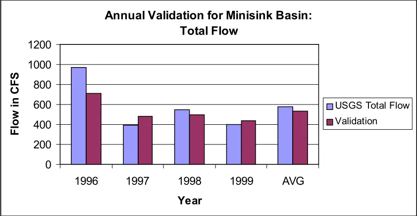
Figure 13: Annual Validation for Minisink Subbasin: Total Flow... 57
Figure 14: Annual Validation for Anamolink Subbasin: Surface Flow... 57
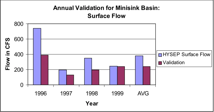
Figure 15: Annual Validation for Minisink Subbasin: Surface Flow... 58
Figure 16: Annual Validation for Anamolink Subbasin: Base Flow... 58
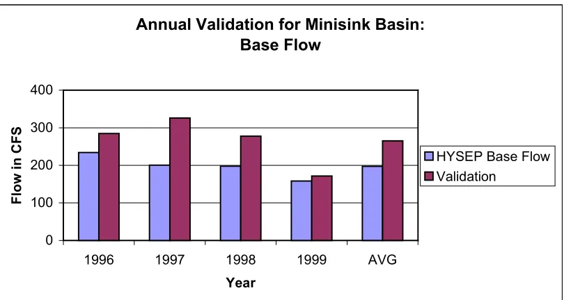
Figure 17: Annual Validation for Minisink Subbasin: Base Flow... 59
Figure 18: Results of Anamolink Monthly Validation, Total Flow... 63
Figure 19: Results of Anamolink Monthly Validation, Surface Flow... 64
Figure 20: Results of Anamolink Monthly Validation, Base Flow... 64
Figure 21: Results of Minisink Monthly Validation, Total Flow... 65
Figure 22: Results of Minisink Monthly Validation, Surface Flow... 66
List of Tables
Table 1: Run Descriptions for Annual Surface Flow Calibration... 47
Table 2: Surface Flow Comparisons for Anamolink, in CFS... 48
Table 3: Surface Flow Comparisons for Minisink, in CFS... 48
Table 4: Run Descriptions for Annual Base Flow Calibration... 49
Table 5: Base Flow Calibration Comparisons for Anamolink Subbasin... 50
Table 6: Base Flow Calibration Comparisons for Minisink Subbasin... 50
Table 7: Run Descriptions for Monthly Surface Flow Calibration... 52
Table 8: Statistics For Monthly Surface Flow Calibration Comparisons of Anamolink Subbasin, All Months... 52
Table 9: Statistics For Monthly Surface Flow Calibration Comparisons of Minisink Subbasin, All Months... 52
Table 10: Statistics For Monthly Surface Flow Calibration Comparisons of Anamolink Subbasin, Non-Winter Months... 52
Table 11: Statistics For Monthly Surface Flow Calibration Comparisons of Minisink Subbasin, Non-Winter Months... 52
Table 12: Statistics For Monthly Surface Flow Calibration Comparisons of Anamolink Subbasin, Winter Months... 53
Table 13: Statistics For Monthly Surface Flow Calibration Comparisons of Minisink Subbasin, Winter Months... 53
Table 14: Run Descriptions for Monthly Base Flow Calibration... 54
Table 15: Statistics For Monthly Base Flow Calibration Comparisons of Anamolink Subbasin, All Months... 54
Table 16: Statistics For Monthly Base Flow Calibration Comparisons of Minisink Subbasin, All Months... 54
Table 17: Statistics For Monthly Base Flow Calibration Comparisons of Anamolink Subbasin, Non-Winter Months... 55
Table 18: Statistics For Monthly Base Flow Calibration Comparisons of Minisink Subbasin, Non-Winter Months... 55
Table 19: Statistics For Monthly Base Flow Calibration Comparisons of Anamolink Subbasin, Winter Months... 55
Table 20: Statistics For Monthly Base Flow Calibration Comparisons of Minisink Subbasin, Winter Months... 55
Table 21: Monthly Validation Statistics For Anamolink Subbasin, All Months... 60
Table 22: Monthly Validation Statistics For Minisink Subbasin, All Months... 60
Table 23: Monthly Validation Statistics For Anamolink Subbasin, Non-Winter Months ... 61
Table 24: Monthly Validation Statistics For Minisink Subbasin, Non-Winter Months.. 61
Table 25: Monthly Validation Statistics For Anamolink Subbasin, Winter Months... 61
Table 29: Monthly Surface Flow Calibration Comparisons of Anamolink Subbasin,
Non-Winter Months... 94
Table 30: Monthly Surface Flow Calibration Comparisons of Minisink Subbasin, Non-Winter Months... 95
Table 31: Monthly Surface Flow Calibration Comparisons of Anamolink Subbasin, Winter Months... 96
Table 32: Monthly Surface Flow Calibration Comparisons of Minisink Subbasin, Winter Months... 96
Table 33: Monthly Base Flow Calibration Comparisons of Anamolink Subbasin, All Months... 97
Table 34: Monthly Base Flow Calibration Comparisons of Minisink Subbasin, All Months... 98
Table 35: Monthly Base Flow Calibration Comparisons of Anamolink Subbasin, Non-Winter Months... 99
Table 36: Monthly Base Flow Calibration Comparisons of Minisink Subbasin, Non-Winter Months... 100
Table 37: Monthly Base Flow Calibration Comparisons of Anamolink Subbasin, Winter Months... 101
Table 38: Monthly Base Flow Calibration Comparisons of Minisink Subbasin, Winter Months... 101
Table 39: Annual Validation Comparison for Anamolink Subbasin, Total Flow... 102
Table 40: Annual Validation Comparison for Minisink Subbasin, Total Flow... 102
Table 41: Annual Validation Comparison for Anamolink Subbasin, Surface Flow... 103
Table 42: Annual Validation Comparison for Minisink Subbasin, Surface Flow... 103
Table 43: Annual Validation Comparison for Anamolink Subbasin, Base Flow... 104
Table 44: Annual Validation Comparison for Minisink Subbasin, Base Flow... 104
Table 45: Monthly Validation Comparisons for Total Flow of Anamolink Subbasin, All Months... 105
Table 46: Monthly Validation Comparisons for Total Flow of Minisink Subbasin, All Months... 106
Table 47: Monthly Validation Comparisons for Total Flow of Anamolink Subbasin, Non-Winter Months... 107
Table 48: Monthly Validation Comparisons for Total Flow of Minisink Subbasin, Non-Winter Months... 108
Table 49: Monthly Validation Comparisons for Total Flow of Anamolink Subbasin, Winter Months... 109
Table 50: Monthly Validation Comparisons for Total Flow of Minisink Subbasin, Winter Months... 110
Table 51: Monthly Validation Comparisons for Surface Flow of Anamolink Subbasin, All Months... 111
Table 52: Monthly Validation Comparisons for Surface Flow of Minisink Subbasin, All Months... 112
Table 55: Monthly Validation Comparisons for Surface Flow of Anamolink Subbasin, Winter Months... 115 Table 56: Monthly Validation Comparisons for Surface Flow of Minisink Subbasin,
Winter Months... 116 Table 57: Monthly Validation Comparisons for Base Flow of Anamolink Subbasin, All
Months... 117 Table 58: Monthly Validation Comparisons for Base Flow of Minisink Subbasin, All
Months... 118 Table 59: Monthly Validation Comparisons for Base Flow of Anamolink Subbasin, Non-Winter Months... 119 Table 60: Monthly Validation Comparisons for Base Flow of Minisink Subbasin,
Non-Winter Months... 120 Table 61: Monthly Validation Comparisons for Base Flow of Anamolink Subbasin,
Winter Months... 121 Table 62: Monthly Validation Comparisons for Base Flow of Minisink Subbasin, Winter
Chapter 1: Introduction and Background Information
Introduction
The Delaware River is approximately 330 miles long and drains roughly 12,675 square
miles of Delaware, New Jersey, New York, and Pennsylvania. It flows from northwest to
southeast, transecting five topographic provinces: The Appalachian Plateau; the Ridge
and Valley Province; the Reading Prong; the Piedmont; and the Atlantic Coastal Plain.
The river’s main stem is unimpeded by dams or control structures as it flows across these
provinces, making it one of the few large free flowing rivers remaining in the contiguous
United States. This “free flowing” characteristic has allowed in excess of 100 miles of
the Delaware River to be designated as National Wild and Scenic Rivers System
(http://www.nps.gov/dewa).
The Delaware River is an irreplaceable natural resource. It provides nearly 10 percent of
the U.S. population with water while covering only 0.4 percent of the country’s land area.
The current water quality conditions of the river are considered above average, and to
maintain this standard the Delaware River Basin Commission (DRBC), the U.S. Army
Corps of Engineers, and state and local authorities have put heavy regulations on land
and water degradation (http://www.nps.gov/dewa).
Three parks encompass approximately 120 miles of the Delaware River: The Delaware
Water Gap National Recreation Area (DEWA), the Middle Delaware Scenic and
Recreational River, and the Upper Delaware Scenic and Recreational River. In
accordance with the regulations issued by the DRBC and the U.S. Army Corps of
an inherent problem with the parks’ ability to meet this mandate. There are over 4,000
square-miles of watersheds contributing flow to these “special protection waters”, of
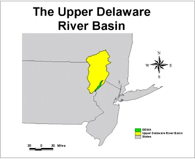
which the parks only manage 110 square-miles. (http://www.nps.gov/dewa). Figure 1
shows the relative size of the upper Delaware River basin compared to DEWA.
Figure 1: The Upper Delaware River Basin
Due to this overwhelmingly large portion of the Upper Delaware River Basin not under
federal or state protection, the personnel at DEWA would like to utilize Geographic
Information Systems (GIS) in conjunction with hydrologic modeling in an effort to help
Background
In the early 1990’s, North Carolina State University (NCSU) began working
cooperatively with DEWA to create a model of the Broadhead watershed. The
Broadhead basin drains approximately 290 square-miles of Monroe and Pike Counties in
North Eastern Pennsylvania. The majority of this watershed lies outside of the park
boundary and consists mainly of forested, rural, and agricultural land. However, there is
some development pressure on the East side of the basin that includes both commercial
and non-commercialization of private lands. Figure 2 shows the Broadhead basin relative
to the Upper Delaware basin and DEWA.
Sung-Min Cho, an NCSU doctoral student, developed the original hydrologic model for
the Broadhead. He tested a series of hydrologic models and concluded the SWAT model
run in ArcInfo to be the most suitable (Cho, 1995). Unfortunately, this program was not
user friendly and needed a great deal of training to be implemented. To try and alleviate
this problem Dr. Casson Stallings created a GUI interface that would allow the majority
of the model to run in ArcView (Stallings, 1998). This program was completed in June
of 1998 and was called SAVI. SAVI was given to the park, but due to changes in park
personnel and project priority the program was not widely utilized.
In the intervening four years, faster computer speeds, greater storage capacities, and more
robust software has raised the potential for more accurate and user-friendly hydrologic
modeling. In addition, personnel changes and more proposed development has led
DEWA to again becoming interested in integrating hydrologic models into the
management of the park’s watersheds.
Project Objective
The objective of this project is to attempt to produce a working model that can accurately
predict flow for the Broadhead basin. This is the first step in developing a complete
hydrologic model that DEWA can utilize to predict and monitor water quality of the
Chapter 2: Literature Review
Introduction to Literature Review
“Prior to the advent of the unit hydrograph by Sherman (1932), hydrologic modeling was
mostly empirical and based on limited data. [In] those days, graphs, tables, and simple
analytical solution were the standard models, and hand calculations, in conjunction with
sliderule, reflected computing prowess” (Singh and Fiorentino, 1996). Since the advent of
the hydrograph, hydrologic modeling has developed into a data intensive, computer
software driven science. Today, there are models covering every facet of water’s
interaction with the environment. As stated in the background section of this paper,
DEWA would like to posses a model that will reasonably predict flow and water quality
changes resulting from development or other land use changes within the basins that flow
into their park. The criteria the park has asked of the model are 1) the capability of
predicting long term effects of changes in land use, 2) fairly easy to use with a quick
learning curve, and 3) able to visually display outputs in map and table form. The
purpose of the literature review is to evaluate the different types of hydrologic models,
compare those models that could be used for the Broadhead basin, and then to provide a
detailed outline of the most appropriate model for the project.
Model Types
Lumped and Distributed models are the two basic types of models used for Hydrologic
Modeling. They can be deterministic or stochastic in nature, meaning the outputs are
for the Broadhead basin and not require any additional data collection and fieldwork,
such as drilling monitoring wells, collecting soil samples, and creating stream profiles.
Lumped Models
Lumped hydrologic models are those models that commonly ignore spatial variations of
precipitation, water flow, and other related processes, focusing instead on spatially
averaged inputs, outputs, and parameter values. Their usefulness is limited due to their
inability to account for the complexities of hydrologic processes and systems. Lumped
models therefore are usually limited to those catchments where spatial variability does
not dictate the outcome of an event (Muszik, 1996).
Distributed Models
“A truly distributed model of a process is possible only if the process can be described by
an equation having an analytical solution” (Muszik, 1996). These types of models are
physically based; meaning they are based on observed parameters rather then estimations.
While the majority of distributed models require some degree of lumping, their objective
is to account for spatial variations of hydrologic processes and parameters. Previously,
limitations of distributed models came from computing the vast amount of data required
to run the model. However, do to advancements in computers and modeling software, the
current limitation for distributed modeling is the lack of available distributed hydrologic
Model Comparisons
Based on the criteria set forth by the park, 11 models were compared.
Flow Models
The first three models, DR3M (Distributed Routing Rainfall-Runoff Model—version II),
GLSNET (Regional hydrologic regression and network analysis using generalized least
squares), and PRMS (Precipitation-Runoff Modeling System), have been grouped
together based on their designation as flow prediction models. All three models are
free-ware and can be downloaded through the USGS website. These models were eliminated
upon first review due to their inability in calculating nutrient predictions, which will
eventually be required.
Flow and Nutrient models
ANSWERS 2000
ANSWERS (Nonpoint Source Nutrient Planning Model) is an event based, distributed
non-point source pollution model. “The model was developed for use by nonpoint source
pollution managers to study the long-term effectiveness of best management practices
(BMPs) in reducing runoff, sediment, and nutrient losses from agricultural watersheds”
(Bouraoui and Dillaha, 1994). It simulates infiltration, evapotranspiration, percolation,
and runoff and losses of nitrate, adsorbed and dissolved ammonium, absorbed total
make up the catchment’s array may not exceed 1 ha, but can be made as small as the
designer wishes.
ANSWERS was run for 25-months on two small watersheds, 1.4 ha and 1.3 ha, near
Watkinsville, GA. It simulated runoff and nutrient loss well without any form of
calibration. The model was then validated on a large watershed, 1153 ha, in Fauquier
County, VA. It was run for five months after the calibration of two sediment detachment
parameters. Predictions of cumulative runoff along with sediment and nutrient losses
were within 39% of observed values. Predictions of individual runoff event losses were
considerably less accurate (Bouraoui and Dillaha, 2000).
While this model seems to predict long term effects reasonably well, its inability to create
cells larger than one ha and its use of an hourly time step exclude it from being used in
this project. ANSWERS is also better suited for strictly agricultural watersheds.
ESWAT
ESWAT (Extended Soil Water Assessment Tool) is an extension of SWAT (discussed in
detail later). Developed by A. van Griensven at the Vrije Universiteit Brussels, ESWAT
is meant to completely model water quality and quantity processes in river basins.
ESWAT models on an hourly time step, introduces reaeration at structures, and has a
multi-objective auto-calibration module. (van Griensven)
ESWAT was not chosen because the extended capabilities of SWAT were of no use to
MIKE SHE coupled with MIKE 11
MIKE SHE is distributed and physically based hydrologic modeling program produced
by the Danish Hydraulic Institute (DHI). Its goal is to allow the user to simulate water,
solutes and sediments in the entire land phase of the hydrological cycle. It has a modular
design that can be used to create an integrated model. Its individual components can be
used together or independently depending on data availability and project goals. Coupled
with MIKE 11, DHI’s one-dimensional model used for channel networks, MIKE SHE
has the power to create an integrated surface water / ground water or drainage system /
ground water model.
MIKE SHE’s basic modular components are pre and post processing (PP), and water
movement (WM). The WM module is the core of MIKE SHE containing several process
simulation modules that when put together describes the entire land phase of the
hydrologic cycle. The WM module components are: evapotranspiration (ET),
unsaturated zone flow (UZ), saturated zone flow (SZ), overland and channel flow (OC),
and irrigation (IR).
MIKE SHE also contains a number of add-on modules to make the program more robust.
The add-on modules are: linear reservoir (LR), advection/dispersion solute transport
(AD), particle tracking (PT), adsorption/degradation (SD), geochemistry (GM),
biological degradation (BM), crop yield and nitrogen consumption (DAISY), macro pore
flow (MP), soil erosion module (SE), soil plant system simulation (DAISY).
MIKE SHE coupled with MIKE 11 was originally chosen as one of the two models for
this program because of its recognition as leading modeling software and their
testing the MIKE SHE/ MIKE 11 software because of its robustness. However, after
attempting to create the input data sets it was realized that MIKE SHE required too much
data and was therefore excluded from the project. MIKE SHE and MIKE 11 are
explained in detail on DHI’s web-site http://www.dhi.dk/index.htm.
WEPP
WEPP (Water Erosion Prediction Project) is a distributed parameter, continuous
simulation, and erosion prediction model. The input parameters include rainfall amounts
and intensity, soil textural qualities, plant growth, plant growth parameters, residue
decomposition, effects of tillage implements, slope shape, steepness, and aspect, and soil
erodibility. WEPP’s strengths lie in modeling field areas that include only ephemeral
gullies and not those catchments that contain permanent channels such as perennial
streams (Becker et al., 1997).
Though WEPP has been validated and tested on numerous sites, it is meant for much
smaller watersheds than that of the Broadhead, and was therefore excluded from the
project.
WMS
The WMS (Watershed Modeling System) is a program containing a suite of hydrologic
models bundled into one user interface. It is produced by a private vendor and can be
Though WMS has a user-friendly interface that utilizes GIS data, its cost, along with its
sole use of HSPF (discussed later) as the complete watershed model, exclude it from
being used in this project.
BASINS
BASINS is also a suite of hydrologic models packaged into one program by the
Environmental Protection Agency (EPA). Its current release is 3.0 and can be
downloaded as free-ware from the EPA’s website, http://www.epa.gov/OST/BASINS/.
It was originally released in September, 1996 with the intention of facilitating the
examination of environmental data, providing an integrated watershed and modeling
framework, and supporting the analysis of point and non-point source management
alternatives. It contains a multitude of hydrologic models used for different aspects in
modeling. Among the models it contains, HSPF and SWAT are the only two relevant to
DEWA at this juncture and they are discussed in detail below.
HSPF
HSPF is a distributed model that is currently free-ware through the USGS. Developed in
the early 60’s, as the Stanford Watershed Model, its current release is version 11. Its goal
is to simulate a number of hydrological processes, listed below, for extended periods of
time. These processes include water quality issues involved with processes on pervious
and impervious land surfaces and in streams and well-mixed impoundments. It uses
records of meteorological phenomenon and continuous rainfall to calculate stream-flow
HSPF simulates interception soil moisture, surface runoff, interflow, base flow, snow-pack depth and water content, snowmelt, evapotranspiration, ground-water recharge, dissolved oxygen, biochemical oxygen demand (BOD), temperature, pesticides, conservatives, fecal coliform, sediment detachment and transport, sediment routing by particle size, channel routing, reservoir routing, constituent routing, pH, ammonia, nitrite-nitrate, organic nitrogen, orthophosphate, organic phosphorus, phytoplankton, and zooplankton. The model can simulate one or many pervious or impervious unit areas discharging to one or many river reaches or reservoirs. Frequency-duration analysis can be done for any time series. Any time step from 1 minute to 1 day that divides equally into 1 day can be used, and any period from a few minutes to hundreds of years may be simulated. HSPF is generally used to assess the effects of land-use change, reservoir operations, point or non-point source treatment alternatives, flow diversions, etc (Flynn et al., 1995).
While HSPF can produce all the necessary outputs required by DEWA, it is data
intensive requiring inputs such as daily dew-point temperature, wind speed, solar
radiation, humidity, and cloud cover. The watersheds entering the park have very little
background data, making it difficult to work with a model like HSPF.
SWAT
The SWAT (Soil Water Assessment Tool) model is a river basin, or watershed, scale
model developed for the United States Department of Agriculture (USDA) Agriculture
Research Service (ARS). It has the capability to be a distributed model if there is enough
detailed data describing the watershed. However, the model also allows the user to lump
information if detailed data is lacking. It requires specific information about weather,
soil properties, topography, vegetation, and land management practices within the
is efficient enough to run for many years. It is a long-term yield model not capable of
detailed single event flood predictions (Arnold et al., 1998).
Though SWAT is considered a distributed and physically based model, it has more of a
quazi-physical base. It utilizes Hydrologic Response Units (HRU’s) to account for a
basin’s spatial variability instead of using a true spatial model. HRU’s work by assigning
characteristics to the basin being modeled by way of weighted percentages. For example,
if a land area equaling 25% of a basin’s area is described as having soil type “x” and land
cover type “y”, the model will attribute that characteristic to the entire basin with a
weighted average of 25%. This quazi-physical based approach allows users to assume in
cases where data is lacking. It is this ability combined with SWAT’s tested use in large,
History of SWAT
Dr. Jeff Arnold developed SWAT in the early 1990’s. It utilizes several ARS models and
is a direct descendant of the SWRRB (Simulator for Water Resources in Rural Basins)
model (Arnold et al., 1990). Specific models incorporated into the original SWAT are
CREAMS (Chemicals, Runoff, and Erosion from Agricultural Management Systems)
(Kinsel, 1980), GLEAMS (Groundwater Loading Effects on Agricultural Management
Systems) (Lenord et al., 1987), and EPIC (Erosion-Productivity Impact Calculator)
(Williams et al., 1984). Since its original configuration it has undergone several
revisions:
· the ability to incorporate multiple HRUs,
· the ability to handle storage of water in the canopy,
· a CO2 component in the crop growth model to handle climatic changes,
· the addition of the Penman-Monteith equation for potential
evapotranspiration,
· the ability to handle lateral water flow through soil,
· the addition of an in-stream nutrient water quality equation,
· the addition of urban build up/wash off equations,
· the addition of bacteria transport routines,
· the addition of the Green & Ampt equation for infiltration, and finally
· the addition of several agricultural management options.
Description of the SWAT Model
SWAT uses the same modeling process developed by Williams and Hann (1973) for
routing runoff and chemicals through a watershed. This modeling process allows a basin
to be subdivided into grid cells or subwatersheds, called HRUs.
The model is divided into subbasin components, channel routing components and
reservoir routing components. Subbasin components describe hydrology, weather,
sedimentation, crop growth, nutrients, pesticides, and agricultural management. Channel
routing components describe channel flood routing, channel sediment routing, and
channel nutrient and pesticide routing. Reservoir routing components describe reservoir
water balance and routing, reservoir sediment routing, and reservoir nutrients and
pesticides. SWAT’s command structure, model components, and subbasin components
can be found in appendices A, B, and C respectively.
The following is a more detailed description of SWAT’s subbasin components, channel
routing components and reservoir routing components. All the material comes from the
SWAT manual (Arnold et al., 1999B) unless otherwise noted.
Subbasin Components
Hydrology
The hydrology model for SWAT is based on the water balance equation:
Equation 1: The SWAT water balance equation
å
=
-+
= t
i
i i i i i
t SW R Q ET P QR
SW
1
)
( (Arnold et al., 1999B)
daily amounts of rainfall, Q represents runoff, ET represents evapotranspiration, P
represents percolation, and QR represents return flow; all units are in mm.
Surface Runoff
This part of the model simulates runoff volume and peak runoff rates from daily rainfall.
Runoff volume is estimated using a modification of the Soil Conservation Service curve
number technique (USDA-SCS, 1972). Peak runoff rates are estimated using a
modification of the Rational Formula. Details on the equations that calculate surface
runoff can be found in the SWAT manual (Arnold et al., 1999B).
Percolation
Flow is predicted through each soil layer in the root zone using a storage routing
technique. Flow may move upward or downward through the soil profile if some soil
layer exceeds field capacity. Downward flow occurs if an unsaturated soil layer lies
beneath a soil layer that has exceeded field capacity. Its rate is regulated by the saturated
conductivity of the soil layer. Upward flow may occur if field capacity is reached in a
lower soil layer. Soil temperature may also affect percolation. Most notably, if a soil
layer has a temperature less than or equal to 0° Celsius, no percolation will be allowed for
that layer.
variations in conductivity, slope, and soil water content. The model also allows upward
flow to an adjacent layer or to the surface.
Groundwater Flow. Groundwater flow contribution to total stream flow is simulated by
creating a shallow aquifer storage (Arnold et al., 1993). Percolation exiting the bottom of
the root zone is recharge for the shallow aquifer. “A recession constant derived from
daily stream flow records is used to lag flow from the aquifer to the stream. Other
components include evaporation, pumping withdrawals, and seepage to the deep aquifer”
(Arnold et al., 1999B).
Evapotranspiration
SWAT provides three options for estimating potential evapotranspiration: Hargreaves
(Hargreaves and Samani, 1985), Priestly-Taylor (Priestly and Taylor, 1972), and
Penman-Monteith (Monteith, 1965).
The model computes evaporation from soils and plants separately as described by Ritchie (1972). Potential soil water evaporation is estimated as a function of potential ET and leaf area index (area of plat leaves relative to the soil surface area). Actual soil water evaporation is estimated by using exponential functions of soil depth and water content. Plant water evaporation is simulated as linear function of potential ET and leaf area index (Arnold et al., 1999B).
Snowmelt
Similar to CREAMS (Kinsel, 1980), SWAT uses a linear function to estimate snowmelt
on days when maximum temperature exceeds 0° C. Estimating runoff from snowmelt is
treated the same as rainfall. However, rainfall energy is set to 0.0 and peak runoff rates
Transmission Losses
Transmissions losses reduce runoff volumes as the flood wave travels downstream.
“SWAT uses Lane’s method described in Chapter 19 of the SCS Hydrology Handbook
(USDA, 1983) to estimate transmission losses. Channel losses are a function of channel
width and length. Both runoff volume and peak rate are adjusted when transmission
losses occur” (Arnold et al., 1999B).
Ponds
The requirements for pond inputs are capacity and surface area. Storage is simulated as a
function of pond capacity, daily inflow and outflow, seepage, and evaporation. In the
scenario of overflow, ponds are assumed to have only emergency spillways.
Weather
SWAT uses precipitation, air temperature, solar radiation, wind speed, and relative
humidity as weather variables. The variables for precipitation and minimum and
maximum daily temperature can be input directly into the model, or can be simulated by
SWAT’s weather generator. Solar radiation, wind speed, and relative humidity are
always simulated.
Precipitation
Air Temperature and Solar Radiation
The maximum and minimum daily air temperature and solar radiation are generated from
a normal distribution that is corrected for wet-dry probability state. The correction factor
is used to increase deviation in temperature and radiation when there is a change in
weather or on rainy days, and decrease deviations on dry days. This is done to maintain
the long-term standard deviations of daily variables.
Wind Speed and Relative Humidity
Using a modified exponential equation, daily wind speeds are simulated using a mean
value of the monthly wind speed. The daily average relative humidity is simulated using
a triangular distribution of the monthly average. The mean daily relative humidity is
adjusted for wet- and dry-day effects just like temperature and radiation.
Sedimentation
Sediment Yield
The Modified Universal Soil Loss Equation (MUSLE) (Williams, 1975) is used to
estimate the sediment yield for each subbasin.
Soil Temperature
The soil surface temperature is estimated using maximum and minimum temperature,
immediately proceeding the day of interest. Damping depth, surface temperature, and
mean annual air temperature is used to simulate the temperature for each soil layer. “The
daily average soil temperature is simulated at the center of each soil layer for use in
hydrology and residue decay” (Arnold et al., 1999B).
Crop Growth
A single model is used in SWAT for simulating all crops. Energy interception is estimated as a function of solar radiation and the crop’s leaf are index. The potential increase in biomass for a day is estimated as the product of intercepted energy and a crop parameter for converting energy to biomass. The leaf area index is simulated with equations dependent upon heat units. Crop yield is estimated using the harvest index concept. Harvest index increase as a non-linear function of heat units from zero at playing to the optimal value at maturity. The harvest index may be reduced by water stress during critical crop stages (usually between 30 and 90% of maturity) (Arnold et al., 1999B).
Nutrients
Nitrogen
The amount of nitrate contained in runoff, lateral flow, and percolation is estimated as
average concentration per volume of water. Leaching and lateral subsurface flow is
treated with the same approach only without the consideration of surface runoff. Organic
nitrogen losses are estimated using a loading function developed by McElroy et al.
(1976) and modified by Williams and Hann (1978) to handle individual runoff events. It
estimates daily organic nitrogen runoff loss based on concentration levels of organic
nitrogen level in the topsoil layer, the sediment yield, and the enrichment ratio. The use
Phosphorus
SWAT uses a concept originally developed for partitioning pesticides into solution and
sediment phases, described by Leonard and Wauchope (Kinsel, 1980), to estimate the
amount of soluble phosphorus in surface runoff. Soluble phosphorus loss occurring in
runoff is predicted using liable phosphorus concentration in the topsoil layer, runoff
volume and a portioning factor. Sediment transport of phosphorus is simulated with a
loading function as described in organic nitrogen transport. The use of phosphorus by
crops is estimated using a supply and demand approach.
Pesticides
SWAT uses GLEAMS (Kinsel, 1980) for the simulation of pesticide transport by runoff,
percolate, soil evaporation, and sediment. “Each pesticide has a unique set of parameters
including solubility, half life in soil and on foliage, wash off fraction, organic carbon
adsorption coefficient, and cost” (Arnold et al., 1999B).
Agricultural Management
SWAT has the ability to rotate up to three crops per year for an unlimited amount of
years. Irrigation, nutrient, and pesticide application dates and amounts can all be input
into the model. For a more detailed description of Agricultural Management functions in
Routing Components
Channel Routing
Channel Flood Routing
SWAT uses a variable storage coefficient method developed by Williams (1969) for
channel routing. Inputs for the model include reach length, channel slope, bankfull width
and depth, channel side slope, flood plain slope, and Manning’s n for channel and
floodplain. Manning’s equation is used to estimate flow rate and average velocity.
Travel time for flow is estimated by dividing channel length by velocity. Transmission
losses evaporation, diversions and return flow are taken into consideration for estimating
the outflow.
Channel Sediment Routing
The sediment routing model has two components, deposition and degradation, that
operate simultaneously. Deposition is based on fall velocity, which is calculated as a
function of particle diameter squared using Stokes Law. “The depth of fall through a
routing reach is the product of fall velocity and reach travel time. The delivery ratio is
estimated for each particle size as a linear function of fall velocity, travel time, and flow
depth” (Arnold et al., 1999B). Stream power, originally defined by Bagnold (1977) as
the product of water density, flow rate, and water surface slope, is the basis for how
SWAT predicts degradation. Williams (1980) later adjusted this prediction by raising
Channel Nutrient and Pesticide Routing
“Currently no transformations or degradation of nutrients or pesticides are simulated in
channels. Soluble chemicals are considered conservative, while chemicals adsorbed to
the sediment are allowed to be deposited with the sediment” (Arnold et al., 1999B).
Reservoir Routing
The model for the Broadhead does not currently have any reservoirs that require this
SWAT Projects
The purpose of watershed modeling is to predict, and hopefully improve, the effects of
management techniques within a watershed area. Arnold et al., (1998) states that
integrated water management can be viewed as a three, or more, dimensional process
centered around the need for water, the policy to meet those needs, and the management
to implement the policy. Grayson et al., (1992) suggested that the analysis of any model
should at least have the following procedures. First, the model should be tested and
calibrated on a wide variety of watersheds with a wide range of conditions. Second,
negative results should be reported along with positive results, and any uncertainty
involved in the model predictions should also be discussed. Finally, the sources and
precision of all the input data should be presented.
Sophocleous et al., (1999) combined SWAT and MODFLOW to create SWATMOD, a
model capable of simulating the surface water, ground water, and stream-aquifer
interactions on a continuous basis. SWATMOD was developed for analyzing conditions
in the Rattlesnake Creek basin during periods of water shortage. The Rattlesnake Creek
basin is an elongated flat basin, measuring roughly 145 km by 25 km, located in
south-central Kansas. A series of trial and error techniques were used to calibrate the model
with measured data for ground water levels, stream flows, and reported irrigation
techniques over a 40-year period (1955 – 1980). The model was then validated using
additional 40-year (1995 – 2034) simulation period using 1994 boundary and land use
conditions, and a repeat of the past 40 years of climatic data to use as baseline data. The
final step was to implement a series of hypothetical management scenarios geared at
reducing and varying current withdrawal rates to run in the model for comparison with
the baseline data. Given model uncertainties, “the interpretations of the model are going
to be much more reliable in a comparative mode, rather than a predictive sense”
(Sophocleous et al., 1999).
In a related study Perkins and Sophocleous (1999) used SWATMOD to examine relative
increases in stream yield due to the restriction of irrigation during periods of drought on
the Lower Republican River Basin in north-central Kansas. The results of the study
showed that tributary flow was the dominant component of stream yield and “that a
reduction of irrigation water use produces a corresponding increase in base flow and
stream yield” (Perkins and Sophocleous, 1999). However, the increase in stream flow
resulting from the restrictions did not appear to restore the minimum desirable stream
flow.
Manguerra and Engel (1998) did a study to show the importance of parameterization for
predicting runoff using SWAT with an emphasis on improving model performance
without resorting to “tedious and arbitrary parameter by parameter calibration.” This
study involved comparing SWAT’s three schemes of decomposition on three watersheds,
3.28, km2, 22.48 km2, and 113.38 km2. The first scheme allowed the user to subdivide a
channels for routing water, sediment, and nutrients. The second allowed the user to
subdivide the watershed into smaller, more homogeneous areas by superimposing a grid.
The third involved using HRU’s, which aggregate areas associated with unique
combinations of soil and land use regardless of their spatial position in the watershed.
The results showed that for the three basins studied, the use of HRU’s was sufficient in
explaining spatial variability. They continued on to say:
Subdividing the watershed into spatially-referenced and individually routed subwatersheds or grid elements may be required only for the following scenarios: in the presence of site-specific water impoundments such as reservoirs or ponds, for large basins, when significant channel abstractions or losses are expected, and in the cases where detailed visualization of the spatial distribution of an output parameter such as runoff or erosion is desired (Manguerra and Engel, 1998).
Arnold and Allen (1996) stated, “it is important to simulate the major components of the
hydrologic budget to determine the impact of proposed land management, vegetative
changes, groundwater withdrawals, and reservoir management on water supply and water
quality.” They also stated the majority of studies completed at the watershed scale often
attempt to measure only one component. Arnold and Allen (1996) used SWAT for
estimating a large portion of the hydrologic budgets for three watersheds in central
Illinois. The basins have areas of 122, 246, and 188 km2 with topography ranging from
level uplands, to gently undulating uplands, to rugged uplands respectively. The land use
for the three watersheds consisted mostly of cropland, pastureland, and woodland. They
validated their multi-component water budget model using field study data collected on
gave reasonable output” and “interaction among the components was realistic” (Arnold
and Allen, 1996).
Arnold et al., (1999) used SWAT for a continental scale simulation of the hydrologic
water balance using soils, landuse, and topography data at a scale of 1:250,000. Water
balance is represented by snow, soil profile, shallow aquifer and deep aquifer. The
hydrologic balance for the contiguous United States was simulated without calibration for
20 years using dominant land use and soil properties for each of the 78,683 polygons.
Long term average annual runoff from USGS stream gage stations were compared to the
simulated average annual runoff for validation.
Results indicate over 45 percent of the modeled U.S. are within 50 mm of measured, and 18 percent are within 10 mm without calibration. The model tended to underpredict runoff in mountain areas due to lack of climate stations at high elevations. Given the limitations of the study (i.e., spatial resolution of the data bases and model simplicity), the results show that the large-scale hydrologic balance can be realistically simulated using a continuous water balance model (Arnold et al., 1999).
SWAT was used by Arnold, Jeffery G. et al. (2001) in a study to asses the ability of
Walker Creek, located near Dallas, TX, in maintaining ample flow to sustain a proposed
bottomland wetland for use in mitigation. A modification to SWAT was made to allow
ponded water within the proposed wetland to interact with the soil profile and shallow
aquifer. The model simulation period was run for 14 years and validated using flow data
from a nearby stream with similar characteristics since there was no available data
available for Walker Creek. Results indicated that the wetland should be equal to or
greater than 85% capacity over 60% of the time, 40% capacity was reached less than 1%
(hydroperiod, soil water storage, plant water uptake) over a range of climatic conditions
and (2) the ability to assess the long-term impact of land-use and management changes”
Chapter 3: Methodology
Overview
In order to apply a model to the Broadhead watershed, the project was separated into
several steps. These included:
· getting the necessary modeling software,
· collecting and manipulating the necessary data for input into the model,
· entering the data into the model,
· running the model,
· handling the model outputs,
· analyzing the model outputs and calibrating the model, and finally,
· validating the model.
The modeling software used for this project included SWAT version 1999B with the
ArcView GIS interface, and HYSEP (Hydrograph Separation Program). SWAT can be
downloaded from the SWAT website http://www.brc.tamus.edu/swat/swatvers.html.
HYSEP is a USGS model used for the separation of total flow into base flow and surface
flow, an important step needed for calibration of the SWAT model. The model can be
downloaded from the USGS website http://water.usgs.gov/software/hysep.html. Both
models are freeware that have been widely used and tested.
The data used for this project included a 30 Meter DEM, a Landuse/ Landcover shapefile,
a STATSGO soils coverage, daily weather data, and USGS gage data. The 30 Meter
Service’s (NRCS) website http://www.ftw.nrcs.usda.gov/stat_data.html. The weather data
was obtained from the U.S. Forest Service weather station, Bushkill Weather Station. The
USGS gage data came from two gage stations, Broadhead Creek near Anamolink and
Broadhead Creek at Minisink Hills, which were retrieved from the USGS website
http://pa.waterdata.usgs.gov/nwis/current?type=flow.
The data was manipulated for input into the SWAT using ESRI’s ArcView 3.2®, ESRI’s
ArcInfo 8.01®, Microsoft Excel 2000®, and Microsoft Access 2000®.
Model output conversions and analysis of results were done in Microsoft Excel and SAS’
Jump 4.0®.
Data Manipulation
The data for this project needed several adjustments in order to be used in the Broadhead.
Since most data was already projected in 1983 Universal Transverse Mercator (UTM)
meters it was decided that this would be projection for all spatial data entered into the
model. SWAT also requires that measured data be in metric units, so unless otherwise
noted all model parameters are metric.
The first step was to create a shapefile of the Broadhead watershed for use in clipping
desired areas. This was done by bringing the 30 Meter DEM into SWAT and utilizing its
stream definition tool to delineate the Broadhead basin (see appendix D). The resulting
shapefile had a 500-meter buffer added to it using ArcView and was saved as
The Landuse/ Landcover shapefile was converted to a grid with cell sizes equaling 30
meters, equal to the DEM.
The STATSGO soil coverage had to be reprojected from 1927 Albers Conical Equal
Area meters to 1983 UTM meters using ArcInfo. It was then converted to a shapefile,
brought into ArcView, and clipped with the brdhdbuff500.shp using the geoprocessing
wizard to cut out all extraneous area not involved in the project. The shapefile was
converted to a grid with a cell size of 30 meters for inclusion into SWAT. The soil
attribute tables necessary for SWAT to function were then built from the .dbf files that
came with the STATSGO download (see appendix E).
The weather data retrieved from the Forest Service was in hardcopy form dating from
January 1, 1993 through October 20, 1999. Daily precipitation in inches and maximum
and minimum temperature in Fahrenheit were entered into an excel spreadsheet. Daily
precipitation was converted to millimeters and maximum and minimum temperatures
were converted from Fahrenheit to Celsius, all values were set to two decimal places.
Using the data from the weather table, a precipitation and a temperature table were made
for inclusion into SWAT. The precipitation table contained a column labeled “DATE”
which contained daily date values, and a column labeled “PCP” which contained daily
values for precipitation in mm. The temperature table contained a column labeled
“DATE” which contained daily date values, “MAX” which contained daily maximum
temperature values in Celsius, and “MIN” which contained daily minimum temperature
in Celsius. The daily values for both tables were extended by copying the data from
January 1, 1993 through December 31, 1995 and pasting them in for the dates of January
through December 31, 1989. This was done get the initial flow conditions to match the
flow at the beginning of calibration period. The end result was a precipitation table and a
temperature table containing daily values for January 1, 1987 through October 20, 1999.
Look up tables were then made so SWAT would be able to call the STATSGO soil
attribute data and the weather data. The STATSGO lookup table contains a field called
“VALUE”, which represents the grid attribute code in the STATSGO soils grid, and a
field called “STMUID”, which identifies the file name for the soil attribute data (see
appendix F). The precipitation look up table contains a field called “ID”, which
represents the weather station, a field called “NAME”, which points to the daily
precipitation table created above, a field called “XPR” which represents the x coordinate
of the weather station, and a field called “YPR”, which represents the Y coordinate of the
weather station (see appendix G). The daily temperature look up table is set up the same
way as the daily precipitation data table, except the “NAME” field points to the daily
temperature file (see appendix H).
In order to calibrate and validate the SWAT model, measured daily flow data from within
the Broadhead basin had to be obtained, separated into base flow and surface flow, and
averaged into annual and monthly values. Since there is not any flow or gage data at the
outlet of the Broadhead, calibrations and validation of the model would have to be done
on smaller subbasins within the Broadhead. The flow data was obtained from the USGS
gage sites Anamolink and Minisink in the form of daily average discharge in Cubic Feet
were set up for inclusion into HYSEP (see appendix I), and then run in HYSEP for
surface flow/ base flow separation (see appendix J) using the local minimum method (see
figure 3).
Figure 3: Local Minimum Method Technique
The outputs from HYSEP for both Anamolink and Minisink were put into their
respective spreadsheets, containing columns for date, total flow in CFS, base flow in
CFS, and surface flow in CFS. The data for total flow and base flow were put into line
graphs for both Anamolink and Minisink and adjustments were made to smooth base
flow where over-estimations occurred in the separation process (see figure 4). These
over-estimations stemmed from high surface runoff over extended periods of time, which
subsequently caused a spike in base flow. The smoothing was done by averaging the
The daily values were then averaged into monthly and annual values for comparison with
the SWAT outputs.
Figure 4: Example of Smoothing Base Flow
Example of Smoothing
0 100 200 300 400 500 600 700 800 900 1000 2/15/1 994 2/22/1 994 3/1/19 94 3/8/19 94 3/15/1 994 3/22/1 994 3/29/1 994 4/5/19 94 4/12/1 994 4/19/1 994 4/26/1 994 5/3/19 94 5/10/1 994 5/17/1 994 5/24/1 994 Date Flow in CFS Total Flow Base Flow Base Flow Smoothed
Finally, the gage locations were needed to properly set up the model so that outputs could
be checked against real data. The USGS websites for the gage stations list the Lat/ Long
coordinates of the gage. These coordinates were entered into a .dbf file, changed to
decimal degrees and added as an event theme in ArcView. The resulting point data was
converted to a shapefile, and then converted to a coverage in ArcInfo. The file was
Folder Structures and File Arrangement
Once all the input data had been placed in proper form, SWAT was an easy model to run
if particular attention was paid to folder structures. First, a folder named “PA” containing
all the STATSGO soil data must be placed into the AvSwatDB\AllUs\statsgo folder
located in the AVSWAT directory (see figure 5).
Figure 5: Folder Structure
This step is very important because SWAT is hard-coded to search for the soil data in this
folder. The rest of the necessary data (the 30 meter DEM, the Landuse/ Landcover grid,
the STATSGO soil GRID, the buffered Broadhead watershed grid, the Gage Station
anywhere in the computers directory structure, however they should be in the same
folder. This is particularly important regarding the precipitation and temperature data
with regard to their look up tables. If they are not in the same folder SWAT will not be
able to find the data.
Setting up the Model
A new project was created in the folder containing all the necessary input data. The
30-meter DEM was loaded into the Watershed, Subbasin and Stream Definition GUI
interface and the projection properties were set to UTM 1983 meters, Zone 18. The DEM
was masked using the buffered Broadhead grid and then preprocessed. In the Stream
definition section, the Threshold Area was set to 30 (ha). This created 1311 outlets/
subbasins. All these outlets were selected and deleted. The gage station shapefile was
added to the view and two outlets were placed corresponding to these points. Eight other
outlets were also placed in the Broadhead basin to separate it into smaller subbasins for a
more accurate model. The outlets were based on natural stream breaks; an attempt was
Figure 6: Broadhead Outlet Locations
This resulted in the separation of the Broadhead into 10 subwatersheds: Two of the
watersheds contributing to the Anamolink gage, eight contributing to the Minisink gage
(the Minisink subbasin includes the two subwatersheds that make up the Anamolink
subbasin), and two subbasins that are ungaged. Figure 7 shows the Broadhead divided
Figure 7: Broadhead Subbasins
The next step required loading the landuse/ landcover grid and the STATSGO soil grid.
This step was completed in the Definition of Landuse and Soil Themes GUI (see figure
8). The landuse/ landcover grid was loaded and pointed to the USGS LULC/ SWAT land
cover table. The SWAT model comes equipped with attribute data for landuse/ landcover
manipulation portion of this section. The lookup table contains an STMUID column, so
the option section on the GUI was set to read STMUID. The lookup table points to the
AvSwatDB\AllUs\statsgo folder located in the AVSWAT directory. If the attribute data
is not placed in this folder the model will not be able to locate the soil information. After
both the landuse/ landcover and the soil grids were loaded, they were merged in SWAT
by using the overlay function in the GUI.
Figure 8: Definition of LandUse and Soil Themes GUI
Before the overlay would run, the model asked for the definition for Multiple Hydrologic
Response Units. Both Land Use (%) over Subbasin Area and Soil Class [%] over
Subbasin Area were set to 5%. This means that any land use or soil class representing
percentage was chosen based on Manguerra and Engel’s finding that “a user who is not
familiar with the spatial nature of the watershed in question should select a fine threshold
area [meaning HRU %] since it does not correspond to a significant increase in
computational time” (Manguerra and Engel, 1998). With the threshold set to 5%, 98
hydrologic response units were created (See Appendix L).
The weather data was then added to the model using the “Weather data definition” GUI
(see figure 9).
Figure 9: Weather Data Definition GUI
The first step required loading the precipitation look up table, created earlier, in the
selected. The “US data base” was chosen because SWAT comes equipped with weather
simulation data for majority of the continental United States, and it is the only data
currently available for this project.
The last step in setting up the model was to have SWAT write all the input files. This
included the watershed configuration file (.fig), the soil data file (.sol), the weather
generator data file (.wgn), the general HRU file (.sub), the main channel data file (.rte),
the groundwater file (.gw), water use data file (.wus), management data file (.mgt), soil
chemical data file (.chm), pond data file (.pnd), and the stream water quality data file
(.swq). The only manual input needed in this section was to set the plant growth heat
units during the writing of the management data file. The option was chosen to use
default values based on local climatic data since no other data was available.
Running the Model
The first step in running the model was to make a decision on the separation of data for
use in calibration and validation. The weather data and USGS gage data obtained for this
project went from January 1, 1993 to October 20, 1999. The three years with the most
flow were 1993, 1994, and 1996. A decision was made to make a separation before 1996
so the calibration data would not contain all the high flow years. The separation was
placed at the end of 1995, effectively making the calibration data run from January 1,
1993 to December 31, 1995 and the validation data run from January 1, 1996 through
October 20, 1999. Once the dates were set for calibration data and validation data the
The first stage was run for calibration of the model on an annual basis. Figure 10 shows
the settings of the annual run for the calibration period. The dates were set so the model
included the priming years and the calibration years of the weather data. The
Penman-Monteith method was chosen based on preliminary runs of the model; it yielded, by far,
the most consistent results to the observed USGS gage flow data. Pesticide outputs and
stream water quality output were not printed because their outputs were not being used in
this project. Channel degradation was set to “Not Active” due to a lack of data. The
model was then run. The initial output was considered as having no-calibration. This data
was put into the conversion spreadsheets and compared against the observed data
(conversions will be discussed in the following section). The model was then calibrated
based on a comparison with the USGS data and run again (calibrations will be discussed
in the following section). This step was repeated until calibration yielded satisfactory
Figure 10: Set Up and Run SWAT Model GUI
The second stage required running and calibrating the model on a monthly time step. All
parameters for the monthly calibration model were set to the same values as the annual
run, except the printout frequency was changed to monthly. The calibration steps were
also handled the same as they were in the annual model, which will be explained in the
following section.
The third and fourth stages required validation of the annual and monthly models. The
model was run on both an annual and monthly time step after changing the last day of
simulation to October 20, 1999. The annual and monthly model outputs for the time
period of January 1, 1995 through October 20, 1999 were then converted to CFS and