PIV Measurements and CFD Simulation of the Performance and Flow Physics and of a Small-Scale Vertical Axis Wind Turbine.

This is a repository copy of PIV Measurements and CFD Simulation of the Performance and Flow Physics and of a Small-Scale Vertical Axis Wind Turbine..

White Rose Research Online URL for this paper: http://eprints.whiterose.ac.uk/80444/

Article:

Edwards, J.M., Danao, L.A. and Howell, R.J. (2013) PIV Measurements and CFD

Simulation of the Performance and Flow Physics and of a Small-Scale Vertical Axis Wind Turbine. Wind Energy. Published online 17 Dec 2013. ISSN 1095-4244,

https://doi.org/10.1002/we.1690

[email protected] https://eprints.whiterose.ac.uk/

Reuse

Unless indicated otherwise, fulltext items are protected by copyright with all rights reserved. The copyright exception in section 29 of the Copyright, Designs and Patents Act 1988 allows the making of a single copy solely for the purpose of non-commercial research or private study within the limits of fair dealing. The publisher or other rights-holder may allow further reproduction and re-use of this version - refer to the White Rose Research Online record for this item. Where records identify the publisher as the copyright holder, users can verify any specific terms of use on the publisher’s website.

Takedown

If you consider content in White Rose Research Online to be in breach of UK law, please notify us by

1. Research Associate, Department of Civil and Structural Engineering, University of Sheffield, Sheffield, United Kingdom. [email protected]

2. Assistant Professor, Department of Mechanical Engineering, University of the Philippines, Quezon City, Philippines. [email protected]

3. Senior Lecturer in Experimental Aerodynamics, Department of Mechanical Engineering, University of Sheffield, Sheffield, United Kingdom. [email protected]

PIV Measurements and ωFD Simulation of the Performance and

Flow Physics and of a Small

-

Scale Vertical Axis Wind Turbine.

Jonathan M Edwards1, Louis Angelo Danao2, Robert J Howell3

Abstract

The aerodynamics generated by a small small-scale vertical axis wind turbine (VAWT) are

illustrated in detail as a NACA0022 rotor blade carries out a complete rotation at three tip

speed ratios. These aerodynamic details are then linked to the wind turbine performance. This

is achieved by using detailed experimental measurements of performance and near blade PIV

and also using a 2D RANS based CFD model. Uniquely therefore, the CFD model is

validated against both PIV visualisations and performance measurements.

At low tip speed ratios ( = 2), the flow field is dominated by large scale stalling

behaviour as shown in both the experimental results and simulations. The onset of stall

appears to be different between the experiment and simulation, with the simulation showing a

gradual separation progressing forwards from the trailing edge, while the experiment shows a

more sudden leading edge roll-up. Overall, similar scales of vortices are shed at a similar rate

in both. The most significant CFD-PIV differences are observed in predicting flow

reattachment. At a higher tip speed ratio ( = 3), the flow separates slightly later than in the

previous condition and as occurs in the lower tip speed ratio, the main differences between

the experiment and the simulation are in the flow reattachment process, specifically that the

simulations predicts a delay in the process. At a tip speed ratio of 4, smaller predicted flow

separation in the latter stages of the upwind part of the rotation is the main difference in

Nomenclature

1

Introduction

In recent years, interest in the VAWT design has been boosted by an increasing desire for the

integration of wind energy into the built environment, where the VAWT presents several

potential advantages over the more common HAWT (horizontal axis wind turbine): the

VAWT avoids the requirement for yaw (turn to face the wind), may have lower sound

emission (due lower tip speed ratio operation, [1]), and shows increased performance in

skewed flow [2] - a likely flow scenario over a roof-top. However, while the HAWT is highly

developed and is currently used for all large-scale wind farms and numerous small-scale

applications in rural locations, the VAWT concept is considerably less-developed.

Simple consideration of the vectors of the blade velocity due to rotation, VB (=R ) and

the freestream velocity, V_∞, yield a skewed-sinusoidal variation of the angle of attack, , with

c blade chord length (m)

Cp power coefficient

Cp-blade power coefficient, blades only

Cp-max maximum power coefficient

L blade length (m)

N number of blades

R rotor radius (m)

T net rotor torque (Nm)

TB blade torque (Nm)

Tres resistive torque (Nm)

VB blade velocity (m/s)

V∞ blade velocity (m/s)

angle of attack rads or deg

c local corrected angle of attack rads or deg

tip speed ratio

azimuth position rads or deg

rotor solidity

changing azimuthal position, . The tip speed ratio, (=VB / V∞), dictates the range in

experienced by the VAWT blade. At a given , the overall performance is the time-averaged

result of the continuously varying aerodynamic forces on the rotor blade within a rotation.

Previous work by the authors [3] has shown that the actual local variation is affected by the

rotor impedance, which increases with tip speed ratio and with increased energy extraction

(higher power coefficient, Cp). Blades in the downstream region also operate in the wake of

the upstream blade passes and the wake of the central drive shaft. Understanding the

operation of a VAWT blade is a very complex problem which requires detailed inspection of

the flow physics. CFD is well-placed to aid the understanding of the VAWT flow physics;

however, the current state of model development is not sufficient to replace experiments [4],

[5], [6], [7].

Much of the knowledge of the stalling process on VAWTs has been developed from lift

and drag polars obtained from pitching aerofoil studies and simulations, Lee [8], [9], [10] and

[11]. This is due to the difficulty of carrying out complex experiments on a rotating turbine.

While aerofoil studies have increased the understanding of stalling behaviour, they are still

limited in their application because they do not reproduce the same flow conditions as found

on VAWTs (lack of wake-wake and wake-support interaction, and a lack of flow induction).

The only other directly relevant studies are due to [12], [13] who also conducted PIV

experiments. Fujisawa and Shiubya [13] conducted experiments at extremely low Reynolds

numbers but described the successive shedding of two pairs of stall vortices from the blade.

The mechanism of dynamic stall was shown to be due to the successive generation of a

separation on the inner surface of the blade followed by the formation of roll-up vortices

from the outer surface. The work by [12] was on a larger VAWT at Re = 5 × 105 and 7 × 105 and  = 2, 3, and 4. Although the convection of the shed vortices away from the blade was

not shown, the roll up and magnitude of the vortices was clearly shown to be effected by ,

with large separations shown at =3 and =2. The flow remained almost completely attached

for the =4 case. Both [12] and [13] showed no corresponding performance measurements so

relation of the dynamic stalling behaviour to performance could not be made.

It is interesting to note that while the fundamentals of the stalling behaviour is not yet

fully understood, some researchers have gone on to develop control methods for the stalling

process, using either synthetic jets [14], or plasma actuators [15] which do show

It remains a fact that, to date, there is simply very little information about the stalling

processes on VAWTs that comes with experimental validation from which the modelling

accuracy can be assessed. This study aims to tackle these pertinent issues. In the following

sections, the development of the CFD model is detailed, as well as the experimental

methodologies. Following this, the aerodynamic and performance measurements are

validated against both experimental PIV visualisations and performance measurements,

which importantly allow the quality of the performance prediction to be assessed with respect

to the simulated flow physics.

2

Methods

2.1

Performance Measurements

2.1.1 Wind Tunnel Facility

All experimental testing was conducted using The University of Sheffield, Department of

Mechanical Engineering’s Low-Speed Wind Tunnel (commissioned in 2011) which is an

open circuit suction tunnel with the flow driven by an axial fan located at the outlet. The

working section is 1.2m wide, 1.2m high and 3m long. The inlet has a two-dimensional

contraction with a ratio of 6.25:1, resulting in a maximum test section velocity of 25m/s and a

turbulence intensity of 0.3% or below over the working region. For these experiments a

turbulence grid was placed at the start of the working section which raised the turbulence

intensity at the turbine to 1%, with approximately 0.01m maximum length scale. This

turbulence intensity was chosen because it allows the turbine to generate both positive

performance at high TSR as well as very well defined vortices and stalling behaviour at low

TSR. Too low turbulence intensity (0.3%) causes negative performance (CP) all throughout

the range of TSR tested, whereas higher turbulence intensity (2.6%) suppressed the formation

of a leading edge separation bubble that would eventually form into the dynamic stall vortex.

2.1.2 Turbine Model

The straight-bladed VAWT rotor (Figure 1) features three NACA0022-profiled blades

each having a chord length, c, of 40mm, and a blade length, L, of 600mm, giving a blade

aspect ratio of 15. Each blade was mounted on two low-drag support arms at the 1/4 and 3/4

blade span positions at a radius, R=0.35m, leading to a solidity, , of 0.34 based on the

conventional definition ( = Nc/R). An optical encoder monitored the rotational speed of the

rotor, which was also fitted with a Magtrol hysteresis brake to provide a known braking

has conflicting suggestions of whether this is significant or not in terms of Cp measurement

[12], [17], [18]. The wind tunnel model is intended to address fundamental understanding of

VAWT performance, and the Cp stated is not intended to represent any particular full-scale

free-operating device. Absolute levels of performance were not important; only relative

values of performance were needed as the paper’s aim is to elucidate the flow physics present

for comparison to an identical computational model.

Figure 1. Wind tunnel arrangement showing the VAWT and PIV system.

The measurement equipment designed by the authors to measure torque was

calibrated giving a maximum error 0.01Nm and corresponds to a maximum error of 5% in

the maximum Cp value determined for tests at 7m/s. The error in measurement of turbine

rotational speed was negligible. The pressure difference measured by the Pitot-static probe

(and a Furness Controls Micromanometer model FC0510) gave an accuracy of the wind

speed measurement estimated at 1.25%. The combined potential maximum error in the Cp

measurement is therefore 7.25%. It should be noted that this is exceptionally accurate for a

system of this scale.

2.1.3 Power Curve Measurement

When testing small wind turbine models, a number of practical problems may be encountered

size. The apparatus, being required to withstand such loading, may give system resistances

which prevent the turbine from ‘cutting-in’. Typically, a VAWT will have a band of for

which positive net torque, T, occurs. Outside of this band, T will be negative and a small

turbine must be driven in order to maintain rotation. Only parts of the T- curve with

negative gradient can be measured without a control system to sense rotational speed and

adjust opposing torque accordingly [17], [19].

The turbine performance is first measured by allowing the rotor to spin down from a high

rotational speed and the deceleration rate monitored using the optical encoder attached to the

hysteresis brake. To fully determine the performance of the rotor blades, two spin down tests

are required for each test condition. The first involves the spin down of the rotor system

without the rotor blades but including the support arms. This is necessary to determine the

system resistance (the drag induced by the support arms, as well as resistance of the bearings

and hysteresis brake etc). It has been determined that the system resistance is independent of

wind speed over the range tested here, i.e. the resistive torque curves from different spin

down tests conducted at different wind speeds are identical [3]. The second spin down test is

conducted with the rotor blades fitted and so measures the full turbine performance. For both

spin down tests, the instantaneous torque is computed by multiplying the instantaneous

rotational deceleration () by the turbine’s rotational moment of inertia (Irig). The rotor blade

torque is then the difference between the rotor torque (TB) and the system resistance (Tres),

see Equation 1. Instantaneous blade power is derived via Eq. 2. This system is used to

determine the performance of the VAWT when it cannot self-sustain itself, i.e. the system

resistance (due to bearing friction, and support arm drag) is greater than the torque developed

by the rotor blades.

B res app rig

T +T +T =I (Eq. 1)

B B

P =T (Eq. 2)

Usefully, this method allows TB to be measured so that the rotor blade performance alone can

be evaluated, see Equation 2 which allows a direct comparison to be made to the 2D CFD

where only the blades are simulated. A detailed assessment of the method can be found in [3].

2.2

PIV Measurements

The flow in the wind tunnel was seeded at the inlet with olive oil droplets approximately 2 m

a Litron Nano L 65-15 Nd:YAG laser (65mJ/pulse) located outside of the tunnel (Figure 1)

on an adjustable height platform. A CCD camera of 1600 x 1600 pixels was used together

with a narrowband greenpass filter to cut-out interference from other sources of light. To

minimise laser light reflection, the blade surface was treated with a Rhodamine 6G-based

paint (produced by the authors). To avoid the support arm obscuring a portion of the field of

view (FOV), the laser sheet was positioned approximately 3c away from the blade tip, and

1.5c away from the support arm. It was confirmed through tests at various positions along the

span that this position was a good representation of the flow along the majority of the blade

length, [19]. For each test, the blade was centered in the reference FOV which was

approximately 140mm x 140mm and the integration area used was 32 x 32 pixels, or 2.8mm

x 2.8mm. The time interval between exposures was set to yield an approximately eight pixel

displacement assuming V= 4 V∞ based on similar tests carried out by Ferreira et al [12]. 100 ensembles were acquired for each condition tested. The measurements concentrated on three

tip speed ratios which were chosen to cover the important and distinct regions of the Cp-blade

curve (Figure 20, discussed later in Section 3.2):

1) = 2 is near the minimum Cp-blade,

2) = 3 is on the part of the curve where the Cp-blade is rapidly increasing,

3) = 4 is near the maximum Cp-blade.

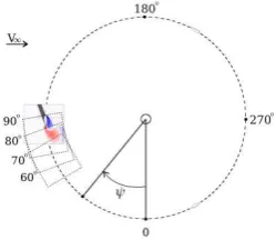
Measurements were taken at 10°intervals in , following one of the rotor blades, for the first

time, through an entire rotation, as illustrated in Figure 2.

Figure 2. PIV results at different  positions showing the rotor blade and FOV.

2.3

CFD Model

The commercial CFD code Ansys Fluent 12.1 was used for all of the simulations detailed in

this study. The Ansys Fluent 12.1 documentation [21] provides details concerning the

otherwise, the recommended values were used for solver settings and model coefficients. The

pressure-based solver was used with absolute velocity and second order implicit transient

formulation. The coupled pressure-velocity scheme was used, and a second order upwind

discretisation was used for all solution variables.

2.3.1 Mesh

Earlier studies [4], [19], [22] have shown that the main flow characteristics of the VAWT can

be represented using a two-dimensional CFD model. Such a model is unable to account for

the effects of the support arms or the blade tip losses on performance; however, this study is

concerned with the dominant flow physics of the VAWT, those are secondary effects. The

computation time for a three-dimensional simulation would be excessive for a study of this

detail.

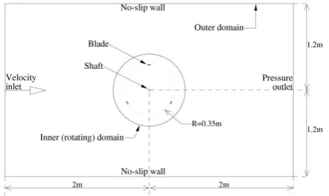
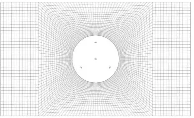
The model domain consisted of two mesh zones: an inner rotor zone and an outer zone

(Figure 3). The mesh of the inner rotor zone rotates together with the blades and the central

shaft. The outer domain is fixed and has a rectangular outer boundary (representing the wind

tunnel) and a hole in the centre which accommodates the inner rotor zone. At each time step,

the solution is interpolated across the sliding interface boundary. The geometry represented a

mid-blade slice of the wind tunnel rotor. The simulation of a simple 2D-slice of the wind

tunnel set-up would result in a significant over-estimation of blockage. A closer blockage

approximation was achieved by matching the ratio of the rotor and wind tunnel widths in the

CFD model to that of the rotor and wind tunnel cross-sectional areas in the experiment.

Figure 3. Construction of the overall two-dimensional computational domain.

A wider refinement of the wake region is necessary to resolve important flow structures,

which arise due to the wide range in . This was most easily accomplished using a structured

towards the inner zone boundaries (Figure 5). The outer domain was meshed with a simple

structured mesh (Figure 6).

Figure 4. The blade ‘O’ type mesh.

Figure 5. One third of the inner rotor mesh.

Figure 6. Outer domain mesh.

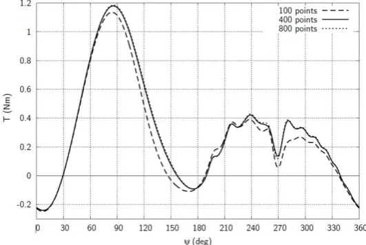
A mesh sensitivity study was conducted to establish the appropriate node density on the

blade surface. Clustering of grid points on the leading edge and trailing edge regions was

implemented to provide enough spatial resolution on these key areas. Wall normal spatial

resolution was fixed starting with a first cell height small enough to result in acceptable y+

levels between 1 to 5 and all solutions were found to have a y+ of below 2.2 [21]. Growth

to be fine enough to provide the required number of layers for boundary layer modelling.

Beyond the near-blade mesh, maximum cell edge length within the central region bounded by

the blade path was studied. It was concluded that the maximum edge length should be limited

to less than half the blade chord to minimise unnecessary dissipation of wake and turbulence

generated by the upwind pass of the blades. Blade torque was monitored for the sensitivity

study. It was found that 400 points around each blade provided the required node density for

accuracy without compromising computational time. A difference of less than 1% in

instantaneous blade torque all around a rotation as can be seen in Figure 7.

.

2.3.2 Turbulence Model Selection

The turbulence model selection was initially carried out by attempting to match flowfield

visualisations and force measurements of a pitching aerofoil study, conducted by [22]. The

range in tested results in the aerofoil undergoing dynamic stall and reattachment, which is

also characteristic of the VAWT and the study therefore represents a simplified test case. It

will be shown later that the excellent matching of the flow physics between the experiment

and the simulations vindicates this approach. Obtaining force data (lift and drag) from a small

VAWT rotor blade is extremely difficult and subject to significant errors [16] so data sets

from pitching aerofoil studies are a useful source for validation. The lift and drag predictions

of the three most suitable models are shown in Figures 7 and 8. Other models were tested

(standard k- , k- , and a laminar solution) but the quality of prediction was found to be poor

and so, for brevity, the results are not presented here.

Figure 8. Lift coefficient results for the turbulence model selection process shown compared

to measurements of a pitching aerofoil study from [8]

Figure 9. Drag coefficient results for the turbulence model selection process shown compared

to measurements of a pitching aerofoil study from [8]

The results of the study showed that the SST k- model gave a the best prediction for the

region of enhanced lift (Figure 8) which occurs due to the roll-up of the leading edge vortex

which is then convected over the aerofoil surface. The early post-stall lift behaviour was also

well-matched for the initial drop in lift occurring as the vortex begins to leave the surface.

While the region of reduced lift and delayed reattachment was over-predicted by all of the

models, the SST k- model was again the closest to the experimental data. Drag prediction

was also well-matched for the increasing region of the pitching motion (Figure 9). Again, all

of the models struggled to accurately simulate the curve hysteresis, with the SST k- model

giving the closest match, particularly in the = 15° to -5° region. It is interesting to note that

better performing that in this case indicating that, perhaps, the pitching blade is an even more

challenging test case.

Plots of the experimental and simulated vorticity flowfields were compared to further

establish the suitability of the SST k- model (Figure 10). Vorticity is plotted here and in

figures which follow because it is a vector field that describes the local spinning motion of a

fluid and is ideal for bringing out details of stalled flow and shear layers.

Figure 10. A plot showing the stream lines for different angles of attack from [8].

Simulations are from the SST k- model showing contours of vorticity.

The complete cycle of the development and shedding of the dynamic stall vortex was

shown to be well-predicted by the model which correctly showed the flow reversal at the

trailing edge, and the subsequent formation of a separation bubble at the leading edge which

rapidly grew and eventually evolved into the dynamic stall vortex that was convected

downstream and finally detached from the aerofoil surface.

Overall, the results of the pitching aerofoil study indicated that the SST k- model is the

best choice for the prediction of the VAWT blade stalling process and it was chosen for all of

the subsequently detailed simulations. This decision is further validated by the closeness with

2.3.3 Time Step and Convergence

The unsteady simulation was stepped forward in time, with up to 50 iterations carried out at

each time step to achieve convergence. The chosen size of the time step and the number of

iterations were a compromise between solution accuracy and computation time. The

rotational position has the most significant influence on the VAWT blade flow physics, and

so the solution was stepped forward using a time interval corresponding to a particular

azimuthal increment angle. A sensitivity study using simulations with different azithumal

angle steps indicated similar torque histories were achieved for time steps which

corresponded to increments of less than 2°. A time step corresponding to an azimuthal

displacement of 0.5°, at the particular being simulated, was therefore chosen as the best

compromise between solution accuracy and computation time, this value was used for all of

the simulations presented in this study. Differences in torque output were less than 1%

between time step corresponding to 0.5 and 1.

The solution was initiated using the inlet velocity value, with a turbulent intensity of 1%

and a length scale of 0.01m defined in order to match the wind tunnel case. A large starting

vortex resulted from the onset of the rotation of the VAWT and a number of rotations needed

to be completed before the initial transients were convected out of the domain.

Figure 11. Torque generated with iteration showing periodic convergence.

The torque curve history for a complete solution shows that convergence of the forces

occurs in around 5 to 10 rotations depending on , see Figure 11. At higher , a higher

number of rotations were completed before periodic convergence was achieved. The solution

residuals were also checked to ensure that they were reduced by 6 orders of magnitude at the

The aim of this study is to show what is possible by using a current commercial CFD

package which is likely to be available to many current design engineers working on VAWT

development. More importantly, this study aims to more fully explain the dynamics of the

flow than has been achieved before and this is necessary for the progression of VAWT flow

understanding and therefore future development.

3

Results

In this section, the results of the CFD simulation with the previously selected turbulence

model are compared against both PIV visualisations and performance measurements. It is the

aerodynamic physics that dictates the turbine performance so it is vital that the two are

understood together. This is the first time this has been carried out in such detail and for a full

rotor revolution over three TSRs. In the first subsection, the simulated and experimental

flowfield is discussed in detail. Contours of vorticity are used to visualise the near-blade

wake, (with the same contour levels maintained for all images). Following this, the

performance of the turbine is analysed in relation to the flow field aerodynamics of both the

simulation and experimental measurement. Differences between the experimental and

computational Cp are also explained.

It should be noted that this paper details significant new results which build upon the

only comparable previous study by Ferreira et al. [12] in which the flow field development

around an entire rotor blade revolution is discussed at a small number of selected locations in

[12]. Differences are expected due to the different solidity and profile the current study uses

the NACA0022, whereas [12] uses the NACA015. The overall blockage between the studies

is very close; currently 29% and 32% in [8].

3.1

Correlation of Experimental and Simulated Flowfields

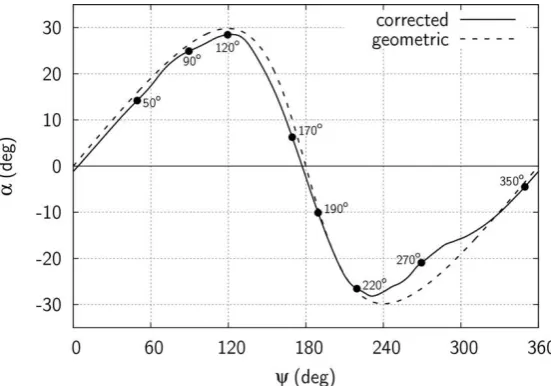
The geometrically derived value of becomes increasingly erroneous as increases due to

the greater impedance which is presented to the flow by the rotor. The rotor exerts a force on

the incoming flow, slowing it down and forcing the streamtube to expand around the turbine,

in order to conserve mass flow rate. To account for this, the discussion of the flow physics

are discussed relative to a corrected angle of attack, c, which has been obtained from the

CFD solution via the method detailed in [3]. For comparison and completeness, the

3.1.1 Flowfield Analysis, = 2

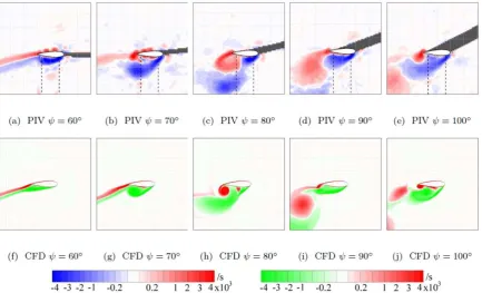
At the = 2 condition, the experimental PIV visualisations shows the onset of stall occurring

around = 60° (Figure 13a), with the first leading-edge vortex leaving the surface at = 70°

where roll-up at the trailing edge is also shown (Figure 13b). The CFD simulation shows a

similar process with a very small lag behind the experiment (Figures 12f and 12g). Figure 12

shows c = 17.3° at = 60°, which is certainly above the static-stall angle. The rapid

increase in c can be thought of as a ‘pitch-up’ motion; in tests on a pitching aerofoil such a

motion is shown to increase the angle of attack at which stall occurs [8]. The simulation

shows the stall process originating from a gradual trailing edge separation; this differs from

the experiment which appears to show a more sudden separation at the leading edge. The

vortex shedding between = 80°, and = 100°, is also similar between the experiment

(Figures 13c to 13e) and the simulation (Figures 13h to 13j), with the simulation continuing

to lag very slightly behind the experimental flowfield.

Figure 13. Plots of vorticity showing the onset of stall, as shown by the PIV measurements and as predicted using the CFD model for  = 2

Towards the mid-rotation point ( = 180°), both the sets of data show a significant

delay in the flow reattachment as the angle of attack rapidly decreases. The simulation shows

quite a sudden change from the shedding of large structures to a much smaller wake (Figures

14f to 14h), whereas the PIV visualisations reveal this to be a more gradual process in the

experiment (Figures 14a to 14c). Either way, this process is likely to keep the performance of

the rotor blade lower than would be the case with a more rapid re-attachment of the flow.

Despite c dropping to 5.9°, the flow has not yet attached by = 170°. As with the

experiment, the reattachment of the flow is shown to occur at around = 190°, where c =

−10.5°. Shortly after this, the flow is shown to stall in the early stages of the downwind part of the rotation. At = 230°, where c has already reached −26.7° (Figure 12), the CFD

simulation shows the flow to be detached (Figure 14i), as did the PIV measurements (Figure

14d). The shedding process is also shown to progress at similar rate between the CFD (Figure

14j) and PIV visualisations (Figure 14e). The rapid decrease in can be thought of as a

‘pitch-down’ motion; in tests on a pitching aerofoil such a motion is shown to lead to a delayed reattachment of the flow as part of the dynamic stall process, which results in

significantly from = 260° onwards (Figure 12), the CFD shows a gradually reducing depth

of stall with the shed vortices also gradually reducing in size (Figures 15f to 15i), which

matches the PIV measurements well (Figures 15a to 145).

Figure 15. Plots of vorticity showing the downwind post-stall vortex shedding and eventual reattachment, as shown by the PIV measurements and as predicted using the CFD model for

 = 2

Understandably, the experimental flowfield varies in this region between rotations

and so the individual vortex positions cannot be matched to the simulation due to the

ensemble averaging of the 100 instantaneous experimental measurements. As a result there is

some smearing of the experimental data. The simulation shows reattachment occurring before

= 350° (Figure 15j), which is in advance of the experimental flow field (Figure 15e). This

would result in lower drag being predicted for this part of the rotation. Averaged around an

entire rotation the performance coefficient is very similar between the experiments and CFD

(Figure 22)

Summary of Simulated Flowfield at = 2

The CFD-simulated flowfield and the PIV visualisations have been shown to be very

well-matched for = 2. The position that the flow detaches from the blade surface is closely

matched for both upwind and downwind parts of the rotation, with only a small delay (<< 10°

in ) being observed for the upwind part. However, the onset of stall appears to be different

between the experiment and simulation, with the simulation showing a gradual separation

progressing forwards from the trailing edge, while the experiment shows a more sudden

leading edge roll-up. The shedding behaviour is also well-matched, with similar scales of

vortices being shed at a similar rate. The most significant CFD-PIV differences are observed

in predicting reattachment: small differences between the experiment and simulation are

observed in the first reattachment at the mid-rotation; however, the simulation predicts the

second reattachment to occur at least 10° in earlier in the rotation when compared to the

experiment.

3.1.2 Flowfield Analysis, = 3

At = 3, the experimental PIV measurements show the onset of separation and subsequent

leading-edge vortex roll-up occurring between = 80° and 90° (Figures 17a and 17b). At the

onset of stall c = 15.2° (Figure 16), which is slightly lower than for = 2 condition; a drop

in the rate of change of angle of attack would be expected to reduce the dynamic stall angle.

Relative to the experiment, the CFD simulation (Figures 17f and 17h) again show a delay in

in , which will result in incorrect lift and drag predictions for this region. Again, the

simulation shows stall beginning with a gradual separation from the trailing edge. The

post-stall vortex shedding is show in the experiments (Figures 17c to 17e) and simulations

(Figures 17h to 17j), with a similar vortex shedding rate observed, and similar reduction in

the depth of stall shown as the angle of attack reduces in this region of the rotation (Figure

16). The 10° in phase difference is maintained for the measurements shown in Figure 17.

Figure 17. Plots of vorticity showing the onset of stall and post-stall vortex shedding, as shown by the PIV measurements and as predicted using the CFD model for = 3

As for the = 2 condition, the reattachment prediction at = 3 is reasonably

well-matched between the experiment (Figures 18a to 18e) and simulation (Figures 18f to 18j).

The gradual reduction in the scale of the shed vortices also appears to be well-matched.

Vortices shed by the upstream blade are visible in the CFD-predicted flowfield at = 190°

(Figure 18j); some trace amounts vorticity of matching sign can also be seen in the equivalent

experimental plot (Figure 18e) but the dissipation and collapse of the vortex structure in the

experiment clearly happens at a faster rate, as would be expected versus a two-dimensional

Figure 18. Plots of vorticity showing the post-stall flow recovery and mid-rotation

reattachment process, as shown by the PIV measurements and as predicted using the CFD model for = 3

Although c reaches a maximum of 16° at = 228°, the simulation predicts the onset

of stall in the downwind portion of the rotation to occur around = 240° (Figure 19f), as do

the PIV measurements (Figure 19a); however, the experimentally observed thicker wake

(relative to attached flow at other positions) indicates partially-separated flow. The extent of

the wake shown in the experiment at = 250° (Figure 19b) further suggests that full

reattachment does not occur around the mid-rotation point. The simulation differs (Figure

19g), instead showing a sudden separation to stall from a fully-attached condition, as was

observed in the upwind part of the rotation (around = 90°). As the angle of attack reduces

significantly beyond = 270° (Figure 16), the simulation shows a gradually reducing depth

of stall with the shed vortices also gradually reducing in size (Figures 19h to 19j), which

matches the experimental measurements well (Figures 19c to 19e). The reattachment of the

flow in the simulation again precedes that which is shown by PIV in the experiment by

Figure 19. Plots of vorticity showing the downwind onset of stall, vortex shedding, and eventual reattachment as shown by the PIV measurements and as predicted using the CFD model for = 3

Summary of Simulated Flowfield at = 3

For the = 3 condition, the position that the flow detaches from the blade surface is slightly

delayed, more so than for the = 2 condition, in both the upwind and downwind parts of the

rotation. The shedding behaviour is again well-matched between CFD and PIV, with similar

scales of vortices being shed at a similar rate. The most significant CFD-PIV differences are

once again observed in predicting the reattachment process: only small differences are

observed in the first reattachment at the mid-rotation point, a much earlier second

reattachment is observed in the downwind part of the rotation, with the simulation showing

earlier reattachment by around 20° in . With a slightly delayed stall and earlier

reattachment, the simulation is likely to over predict the performance measured in the

experiment, this is indeed the case as shown later in Section 3.2.

3.1.3 Flowfield Analysis, = 4

At this condition, the turbine is generating power so more attached flow is likely to be seen in

both the simulations and experimental data. Later detachment of the flow is seen now, from

between = 110° and = 120° where the CFD simulation shows a gradual detachment

experiment (Figures 21a and 21b). However, as the angle of attack reduces beyond as the

rotor reaches = 130°, the simulation (Figures 21h and 21i) does not show the same vortex

shedding as is shown in the experimental flowfield observations (Figures 21c and 21d).

Figure 20 shows that c has already peaked = 105° however, at = 130° c is beginning to

drop rapidly and, in the experiment, a large vortex rolls up in the already separated flow as

the ‘pitch-down’ motion occurs. In the experiment, the stalled flow eventually reattaches around = 180° (Figure 21e), but no large separation is shown in the CFD and the separation

point simply retreats back toward the trailing edge as the angle of attack reduces (Figures 21d

to 21e). As a result, the simulated drag between = 130° and 180° will be significantly

higher than the experimental case, and the lift significantly lower. This is shown in the

performance results at this TSR (see Figure 22) although the performance difference is also

due to 3 dimensional effects not present in the CFD. Due to the significantly reduced relative

velocity in the downwind part of the rotation, the range in  is greatly reduced (Figure 20),

and attached flow is shown for all of the downwind part of the rotation.

Figure 21. Plots of vorticity showing the onset of stall, brief vortex shedding, and subsequent flow recovery as shown by the PIV measurements and as predicted using the CFD model for

 = 4

Summary of Simulated Flowfield at = 4

The lack of a flow separation in the latter stages of the upwind part of the rotation is the only

main point to note when comparing the flowfields of the simulation and experiment for the

= 4 condition. The performance in this region of the rotation would certainly be very different

between the CFD simulation and the experiment, with the simulation very likely to be

predicting lower drag and higher lift than would be actually be experienced by the blade in

the wind tunnel experiment. For the rest of the rotation, the flow is attached in both the

simulation and experiment due to the lowered angle of attack.

3.2

Linking Experimental and Simulated Performance

Comparison of the CFD-simulated flowfield with the experimental observations by PIV has

revealed a good match between the two, showing that it is possible to simulate the basic

VAWT blade flow physics, which includes dynamic stall and reattachment. A good

representation of the general flow physics is an important step towards a useful CFD VAWT

model; however, a correct Cp prediction is likely to be the ultimate goal for most future

experiment is made by adding Cp values from additional simulations to map-out the full

curve.

Results of the CFD-predicted performance are shown alongside the experimental

measurements in Figure 22. The first, and most obvious observation is that the maximum Cp

is over-predicted in the simulation by a significant margin, but this is expected as the 2D

simulation does not include all of the losses that exist in the experiment (which is of course

3D) such as those due to blade tip effects and the interaction between the blades and the

supporting structure. The simulation predicts C_p−max=0.36, whereas the experiment has measured Cp−max = 0.14, clearly the predicted blade forces are quite different between the two cases. However, it should be noted that from the perspective of this study the shape curve

shape is well represented and that is most important: from = 1 the Cp drops to form a

negative trough in the performance curve just above = 2, and from here performance

rapidly improves with increasing with both CFD and experiment crossing to positive Cp at

similar until a maximum Cp is encountered in both cases at around = 4 after which, with

further increases in , a steep drop in performance in experienced.

Figure 22. Cp−blade vs  as predicted by the CFD simulation and as measured in the

experiment

The simulated Cp matches the experiment closely for low tip speed ratios, and the

flowfield has previously been shown to compare well compared for = 2. However, the

increased. Increased stall delay and earlier flow reattachment were observed at =3, and

understandably the CFD predicts higher Cp at this tip speed ratio. Most significantly, no

separation at all was predicted for =4, which would be expected to lead to a significant

over-estimation of Cp at this condition. Certainly, some differences are expected due to 3D

effects: a similar comparison between experiment and 2D CFD has been shown by [7], whose

blades had a similar aspect ratio of 17. Further to this, [18] show a much improved match

between experimental results and their 3D CFD simulations while the equivalent 2D CFD

results were shown to give substantial over-prediction. However, the model turbine used by

Howell et al. had a very low aspect ratio of 4 (in this study it is 15), and so the substantial 2D

CFD versus 3D CFD differences are not surprising. Induced drag effects increase with the

square of lift, and so the wing-tip effect would be expected to become more significant as the

blade reaches an optimum and the blade spends more of the rotation at a high-lifting

condition. Results obtained by [23] have shown an increased effect of aspect ratio with ,

with a change in aspect ratio AR from 160 to 15 leading to an approximate Cp drop of 1/3 at

= 5 and only 1/5 at = 3. This may, in part, account for why the flowfield visualisations

match-up reasonably well, yet the Cp prediction does not. Further to this, a poor prediction of

zero-lift drag, which has the most influence at high [23] where the range in is lowest,

may also be the cause of differences. Additional investigations would be required to better

evaluate the model’s ability to correctly predict the viscous drag, the contribution of which is

most significant at low angle of attack.

4

ωonclusion

The comparison of the CFD-simulated and experimental flowfields have shown a good match

at the three different tip speed ratios tested. The basic process of attached flow, stall, vortex

shedding and reattachment is shown for the = 2 and 3 conditions, although the brief stall at

= 4 is missing in the simulations. A small delay in detachment and earlier reattachment is

shown in the simulation, indicating that the CFD-simulated flow is generally more inclined to

be attached to the blade surface.

Significant differences between simulated and experimental Cp is noted at higher .

However, in general, the performance curve is well-formed, with the same basic trends

observed with changing (albeit they are scaled by larger amounts) and the gradients in the

curve at each of these points are very similar. This all suggests that similar fundamental

both the simulation and the experimental case. Further work is required to assess the impact

of three-dimensional effects on VAWT performance, particularly at higher tip speed ratios,

this being crucial to correct prediction if aiming to realise any real-word device.

Based on the results and analysis in this study, the continued use of the CFD model is

well-justified, particularly where supplemented with experimental data for validation.

Acknowledgements

The authors would like to thank the workshop technicians at the Department of Mechanical

Engineering for the manufacture of the turbine and all the associated measurement

subsystems. For funding this research, Jonathan Edwards would like to thank the University

of Sheffield Studentship Program and Louis Danao would like to thank the Engineering

Research and Development for Technology Program of the Department of Science and

Technology through the University of the Philippines’ College of Engineering.

References

[1] Iida, A., Mizuno, A., and Fukudome, K., 2007, “Numerical Simulation of Unsteady Flow and Aerodynamic Performance of Vertical Axis Wind Turbines with LES,” 16th Australasian

Fluid Mechanics Conference, Gold Coast, Australia, pp.1295-1298.

[2] Mertens, S., Van Kuik, G., and Van Brussel, G. J. W., 2003, “Performance of a High Tip

Speed Ratio H-Darrieus in the Skewed Flow on a Roof,” 41st AIAA Aerospace Sciences

Meeting and Exhibit, Reno, Nevada, USA. AIAA-2003-0523.

[3] Edwards, J. M., Danao, L. A., and Howell, R., 2012, “Novel Experimental Power Curve

Determination and Computational Methods for the Performance Analysis of Vertical Axis

Wind Turbines,” Journal of Solar Energy Engineering, Volume 134, Issue 3, 2012.

[4] C J Simao Ferreira, C. J., van Brussel, G. J. W., and van Kuik, G., 2008, “2D CFD

Simulation of Dynamic Stall on a Vertical Axis Wind Turbine: Verification and Validation

[5] Tullis, S., Fiedler, A., McLaren, K., and Ziada, S., 2008, “Medium-Solidity Vertical Axis Wind Turbines for use in Urban Environments” 7th World Wind Energy Conference,

Kingston, Ontario, Canada.

[6] Raciti Castelli, M., Englaro, A., and E Benini, E., 2011, “The Darrieus Wind Turbineμ

Proposal for a New Performance Prediction Model Based on CFD” Energy, 36(8)μ4λ19-4934.

[7] Wang, S. Hughes, K.J., Ingham, D.B., Ma, L.a, , Pourkashanian, M. and Tao, Z. Edwards,

J.M., Howell, R.J., Danao, L.A.M., Sobotta, D., Qin N. “An experimental investigation into

the aerodynamics of a vertical axis wind turbine using PIV” Under review with the Journal of

Wind Energy and Industrial Aerodynamics.

[8] Lee, T., and Gerontakos, P., 2004, “Investigation of Flow over an Oscillating Airfoil”,

Journal of Fluid Mechanics, 512:313-341.

[9] Mccroskey, W. J., 1981, "The Phenomenon of Dynamic Stall," Technical Report No.

NASA TM-81264, Ames Research Center, Moffett Field, California.

[10] Mclaren, K., Tullis, S., and Ziada, S., 2011, "Computational Fluid Dynamics

Simulation of the Aerodynamics of a High Solidity, Small-Scale Vertical Axis Wind

Turbine," Wind Energy, 15(3), pp. 349-361.

[11] Wang, S., Ingham, D. B., Ma, L., Pourkashanian, M., and Tao, Z., 2010, "Numerical

Investigations on Dynamic Stall of Low Reynolds Number Flow around Oscillating Airfoils,"

Computers and Fluids, 39(9), pp. 1529-1541.

[12] Simao Ferreira, C. J., Van Kuik, G., Van Brussel, G. J. W., and Scarano, F., 2009,

“Visualization by PIV of Dynamic Stall on a Vertical Axis Wind Turbine,” Experiments in

Fluids, 46(1), pp. 97-108.

[13] N Fujisawa and SShibuya. Observations of Dynamic Stall on Darrieus Wind Turbine

Blades. Journal of Wind Engineering and Industrial Aerodynamics, 89(2001):201-214, 2000.

[14] Yen, J. , Ahmed, N.A., “Enhancing vertical axis wind turbine by dynamic stall control

using synthetic jets”, Journal of Wind Engineering and Industrial Aerodynamics, Volume 114, March 2013, Pages 12-17

[15] Greenblatt, D., Ben-Harav, A., Schulman, M., “Dynamic stall control on a vertical axis

wind turbine using plasma actuators ( Conference Paper ) “ 50th AIAA Aerospace Sciences Meeting Including the New Horizons Forum and Aerospace Exposition, 2012, Article

number AIAA 2012-0233

[16] J. H. Strickland, B. T. Webster and T. Nguyen. A Vortex Model of the Darrieus Turbine:

[17] Van Bussel, G. J. W., Polinder, H., and Sidler, H. F. A., 2004, “The Development of

Turby, a Small Vawt for the Built Environment,” Global Windpower 2004 Conference and

Exhibition, Chicago, IL, USA, pp. 10.

[18] Penna, P., and Bertenyi, T., 2008, “Full-Scale Wind Tunnel Testing of the QR5 Vertical

Axis Wind Turbine,” 46th AIAA Aerospaces Sciences Meeting and Exhibit, Reno, Nevada,

USA.

[19] Howell, R., Qin, N., Edwards, J., and Durrani, N., 2010, “Wind Tunnel and Numerical

Study of a Small Vertical Axis Wind Turbine,” Renewable Energy, 35(2), pp. 412-422.

[19] Edwards, J. E., “The Influence of Aerodynamic Stall on the Performance of

Vertical Axis Wind Turbines”, PhD thesis, Department of Mechanical Engineering, University of Sheffield.

[21] ANSYS Inc. Fluent 12.1 user guide and manual. Released 01/10/2009.

[22] Hamada K, Smith TC, Durrani N, Qin N, Howell R. Unsteady Flow Simulation and

Dynamic Stall Around Vertical Axis Wind Turbine Blades. 46th AIAA Aerospaces Sciences

Meeting and Exhibit. Reno, Nevada, USA 2008.

[23] McIntosh, S. C., 200λ, “Wind Energy for the Built Environment” PhD thesis,