Precision Fabrication and Development of Charging and Testing Methods of Fixed-Abrasive Lapping Plates

ABSTRACT

Kametz, David Austin. Precision Fabrication and Development of Charging and Testing Methods of Fixed-Abrasive Lapping Plates. (Under the direction of Dr. Thomas A. Dow.)

PRECISION FABRICATION AND DEVELOPMENT OF CHARGING

AND TESTING METHODS OF FIXED-ABRASIVE LAPPING PLATES.

by

DAVID AUSTIN KAMETZ

In partial fulfillment of the requirements for the Degree of

MASTER OF SCIENCE IN MECHANICAL ENGINEERING

North Carolina State University

2002

APPROVED BY:

________________________________ _________________________________

BIOGRAPHY

ACKNOWLEDGMENTS

There are many people who guided me through my time in graduate school. The patience

and support of all of those around me have been a tremendous help. I would like to

individually thank:

• My Mom, Carole Kametz. Her belief that I can do anything made me confident and determined enough to get through graduate school, and will carry on through life.

• Dr. Thomas A. Dow, my advisor, for taking me under his wing and being an excellent mentor.

• IBM Corporation and John Herber, Rick Singh, Donnie Moorfield and Byoung Loh for their support of the center and my project.

• My other committee members for their help and guidance: Dr. Scattergood and Dr. Eischen.

• Alex Sohn and Ken Garrard for their supreme knowledge of everything I needed help with.

• My family and friends: my brother Tom Kametz, my father Tom Kametz, and friends Stuart Clayton, David Gill, Jordan Green, Matias Heinrich, Andrew Hinkley, David

Hood, Cosmo Lovecchio, Nobu Negishi, Witoon Panusittikorn, Jason Theiling, Kenji

Toda and Lindsay Zych.

TABLE OF CONTENTS

LIST OF TABLES………..vi

LIST OF FIGURES………...vii

LIST OF SYMBOLS AND ABBREVIATIONS ……….xi

CHAPTER 1 Introduction ……….1

1.0Background………..………1

1.1Plate Composition ……….………..5

1.2Current Lap Fabrication Process……….……….6

1.3Lap Plate Examination ………...……….………9

1.3.1Light Microscope………..………..9

1.3.2Talysurf Profilometer………11

Analysis of Talysurf Traces………..14

Peak-to-Valley and RMS Roughness ……….16

Skewness………18

Kurtosis ………19

Bearing Ratio ………20

Peak Spacing ……….21

1.3.3Scanning Electron Microscope ……….23

1.4Current Lap Fabrication Process Problems………25

CHAPTER 2 New Plate Texturing Procedure…………..………..27

2.0 Spiral Groove……….27

2.1 Grooving Parameters ……….27

SEM Micrographs………30

2.1.1 Film Thickness Model ……….32

Estimated Lapping Lift Forces………39

Variable Land Ratio………...39

Variable Groove Depth ………..40

Variable Groove Pitch………41

Estimated Lapping Drag Forces………..43

Variable Land Ratio………...44

Variable Groove Depth ………..45

Variable Groove Pitch………45

2.1.2 Groove Tool Geometry Effects On Machining……….47

Dead Sharp Tool………..48

Round Nosed Tool………51

2.2 Ring Charging and Plate Flatness ………..………53

3.1 Contact Pressure ………58

3.2 Roller Assembly……….61

3.3 Roller Experiments ………62

3.3.1 Roller Material Porosity………63

3.3.2 Roller Flatness ………..65

3.4 Final Assembly Results ……….67

New Slurry Chemistry ……….69

3.4.1 Initial Charging Performance………70

3.4.2 Faced Land Charging Performance………...72

3.4.3 Diamond Concentration vs. Charging Time ……….74

3.5 Roller Charging and Plate Flatness………76

CHAPTER 4 Lapping Performance……..………..79

4.0 Lapping Performance……….80

CHAPTER 5 Friction Tests………..………82

5.0 Test Apparatus……….………...82

5.1 Load Cell Test Error Sources ………86

5.1.1 Level ……….86

5.1.2 Initial Stage Direction ………..88

5.1.3 Translation Stage Velocity………89

5.2 Friction on a Textured Plate………..……….91

5.3 Friction on a Grooved Plate ………..………92

5.3.1 Alumina Charging Ring………92

5.3.2 Alumina Roller Charging ……….93

5.4 Discussion ………..95

CHAPTER 6 Tribometer………..………98

6.0Tribometer Design ………98

6.1Eddy Current Brake ……….………..99

6.2Optical Encoder & Output Program……….………101

6.3Tribometer Performance ………..105

6.3.1Brake Calibration………105

6.3.2Test Trials………110

6.4 Discussion ………114

CHAPTER 7 Conclusions………..……….………117

7.0Conclusions…………..….………..…….117

LIST OF REFERENCES………120

LIST OF TABLES

Table Number Page Number

Table 3.1 Summary of charged area density for various fabrication processes ………….75 Table 6.1 Predicted counts for various friction coefficients and radial positions

using theoretical brake torque………..104 Table 6.2 Predicted counts for various friction coefficients and radial positions

using calibrated brake torque………...111 Table 6.3 Actual encoder counts and roller velocities for roller charging tests

LIST OF FIGURES

Figure Number Page Number

Figure 1.1 Hard disk drive………..………2

Figure 1.2 Illustration of loose-abrasive lapping and fixed-abrasive lapping………3

Figure 1.3 Plates used during study – 12 plugged Mainz tin & 28 plugged high purity tin and Mainz tin ……….………6

Figure 1.4 Illustration of texturing ring on the lapping plate ……….………7

Figure 1.5 Illustration of alumina charging ring on the lapping plate ………..….……8

Figure 1.6 Light microscope image of textured specimen A3 at 50x and 500x ……....…..10

Figure 1.7 Light microscope image of textured specimen B3 at 50x and 500x…………...10

Figure 1.8 Groove orientations created by texturing ring ………..……..11

Figure 1.9 Talysurf profile of textured surface of plug A3 in Figure 1.6 in the X direction ………...…………...….12

Figure 1.10 Talysurf traces of specimen A3 in the X and Y directions over a similar length to that depicted in the 500x micrographs of Figures 1.6 and 1.7 ………...…………..……..13

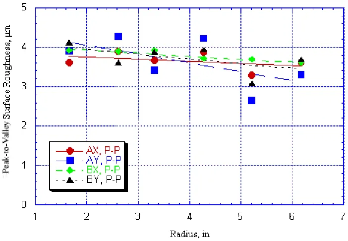
Figure 1.11 Peak-to-Valley surface roughness for all of the plate plug specimens vs. radius………...16

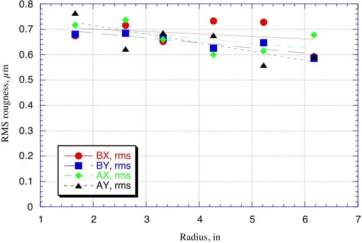
Figure 1.12 RMS average roughness of the plate plugs as a function of radius ..…………..17

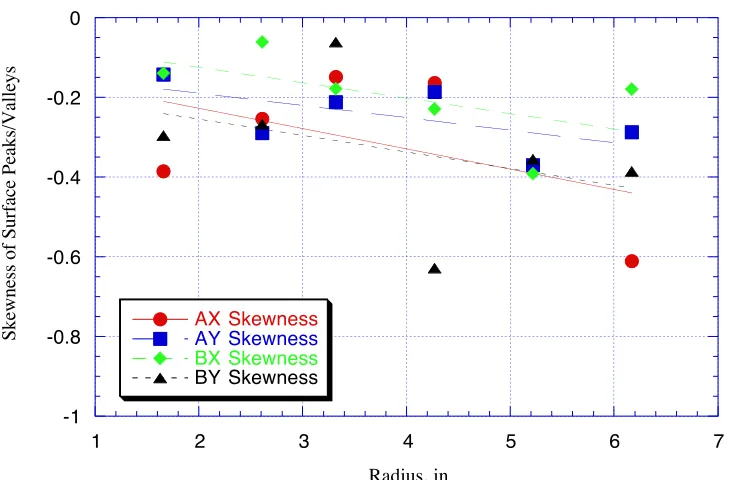
Figure 1.13 Skewness of the peaks and valley as a function of the plate radius……..……..18

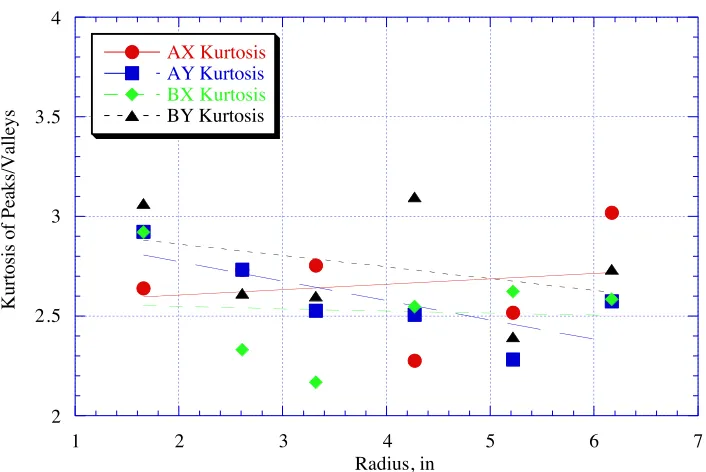
Figure 1.14 Kurtosis of the peaks and valleys as a function of plate radius ………….…….19

Figure 1.15 Bearing Ratio at one RMS from the mean surface ……….……20

Figure 1.16 Average spacing of adjacent peaks on the specimen surfaces ………….……..21

Figure 1.17 Average spacing of the more significant peaks that pass through the mean line………...………...22

Figure 1.18 100x image of the textured surface showing the overall features ………..……23

Figure 1.19 1000x image of the surface showing plateau between grooves …………..…...24

Figure 1.20 3000x image of the plateau showing individual diamond grains ………...25

Figure 2.1 Definition of geometrical parameters of the grooved plate ………28

Figure 2.2 Talysurf of grooved plate after grooving………...……..…………..…….29

Figure 2.3 Talysurf of grooved plate after charging ……….……...30

Figure 2.4 100x SEM images of grooved tin lap plate before charging and after charging ……….……..30

Figure 2.5 1000x SEM images of grooved plate before charging and after charging ………..……….31

Figure 2.6 3000x SEM images of grooved plate before charging and after charging ………..……….31

Figure Number Page Number Figure 2.8 Pressure distribution and definition of the parameters pertinent to the

hydrodynamic force generation of a step bearing …………..……..………...34 Figure 2.9 Wedge bearing geometry ………36 Figure 2.10 Approximate pressure distribution of triangular bearings (solid line)

and slight variance geometries……….37 Figure 2.11 Estimated hydrodynamic lift force versus land ratio for a grooved

plate ……….39 Figure 2.12 Estimated hydrodynamic lift force versus groove depth for a grooved

plate ……….40 Figure 2.13 Estimated hydrodynamic lift force versus groove pitch for a grooved

plate………..……….………...42 Figure 2.14 Estimated hydrodynamic frictional force versus land ratio for a

grooved plate ………..………..…………...44 Figure 2.15 Estimated hydrodynamic frictional force versus groove depth for a

grooved plate………...……….45 Figure 2.16 Estimated hydrodynamic frictional force versus groove pitch for a

grooved plate ……….………..46 Figure 2.17 Tool geometry ………..………..47 Figure 2.18 Tin plate surface grooved with dead sharp tool………..………....48 Figure 2.19 SEM imaging of tin surface features created by dead sharp tool at

200x and 600x ……….………49 Figure 2.20 Tetragonal crystal structure and cubic crystal structure ……….50 Figure 2.21 Illustration of various burr sizes for varying grain orientations ……….51 Figure 2.22 Comparison of the depth of cut with a dead sharp tool and a round

nosed tool……….……….………...51 Figure 2.23 Polynomial fit lines of plate profile of different stages in fabrication…………53 Figure 2.24 Profile of grooved plate before charging ………54 Figure 2.25 SEM images of alumina ring charged tin surface at radial locations

83 mm and 125 mm ……….55

Figure 3.1 Illustration of the new charging technique using a cylinder to roll the

diamond grains into the grooved tin plate…………..………..56 Figure 3.2 Illustration of roller charging mechanism ………..57 Figure 3.3 Illustration of different length cylinders on a flat with sample plots of

stress distribution along the length of the interface ……….58 Figure 3.4 Yield profiles of tin at edge of roller contact under various normal

loads ……….60 Figure 3.5 Yield depth of tin at center of roller contact under various normal

loads ……….61 Figure 3.6 Cross-sectional drawing of roller assembly………62 Figure 3.7 Three-dimensional view of roller assembly………62 Figure 3.8 1000x image of CoorsTek roller charged surface with 17.6 N normal

Figure Number Page Number Figure 3.9 Images of CoorsTek roller charged surface with 27.4 N normal load

at 1000x and 2000x charged for 60 minutes ………...64

Figure 3.10 Talysurf profile of CoorsTek alumina roller ……….………….65

Figure 3.11 SEM image of light region and dark region after 30 minutes of charging using a silicon nitride roller at a normal load of 15.15 N ………….66

Figure 3.12 Silicon nitride roller profile and plate appearance after charging ……….…….67

Figure 3.13 Talysurf profile of HIPed alumina roller ………68

Figure 3.14 Illustration of roller charging mechanism with counterbalance ……….69

Figure 3.15 Images of charged surface with 7.3 N normal load at 500x and 2500x - Stationary roller - 10-minute charge………..70

Figure 3.16 Images of charged surface with 5.5 N normal load at 500x and 2500x - Traversing roller - 60-minute charge……….71

Figure 3.17 Plate appearance after charging grooved plate with HIPed roller after 60 minutes of charging……….72

Figure 3.18 250x image of grooved plate followed by a deep facing cut ……….………….73

Figure 3.19 SEM images of plate surface after land-facing cut at 500x before charging and at 1000x charged 10 minutes with 5.5 N load -Traversing roller………...73

Figure 3.20 Plate appearance after charging with HIPed roller of land-faced grooved plate after 60 minutes of charging ……….…………74

Figure 3.21 Images of charged surface with 5.5 N normal load at 2500x after 10 minutes and 30 minutes of charging – Traversing roller ……….75

Figure 3.22 Polynomial fit lines of plate profile of different stages in fabrication…………77

Figure 3.23 SEM images of tin surface charged with HIPed roller at plate radius locations 50 mm and 120 mm ……….78

Figure 4.1 Vacuum chuck, foam pad and AlTiC strips ……….………..79

Figure 4.2 Lapping plate lapping regions and direction ………..79

Figure 4.3 Material removal rates for various charging mechanisms and charging times………..81

Figure 5.1 Illustration of load cell mounting blocks and AlTiC mounting pad …………..83

Figure 5.2 3-Axis load cell friction testing setup ………84

Figure 5.3 Plate friction testing locations with exaggerated spiral groove ………..84

Figure 5.4 Initial output data for a grooved plate charged for 60 minutes ………..………86

Figure 5.5 Load cell setup at defined angle α ……….87

Figure 5.6 Load cell output for varying tilt angles………..………….88

Figure 5.7 Load cell output for opposite starting velocity directions ……….……….89

Figure 5.8 Load cell output for varying translation stage velocities………..………..90

Figure Number Page Number Figure 5.10 Friction coefficient versus charging time measured at the chord and

radius of a grooved plate charged with the alumina charging ring……..……93

Figure 5.11 Friction coefficient versus charging time for a plate charged with HIPed alumina roller with a normal load of 5.5 N ………..…………94

Figure 6.1 Illustration of eddy current brake and roller assembly ……….…………..99

Figure 6.2 Eddy current brake geometrical parameters ……….100

Figure 6.3 Predicted output counts for a 1.0 second sample time at a plate radial location of 25 mm and 150 mm using theoretical brake torque ………..….103

Figure 6.4 Illustration of brake calibration test setup ………106

Figure 6.5 Non-braked roller velocity versus time with brake off and brake on ……..…107

Figure 6.6 Bearing torque versus roller velocity of three no-braked roller tests and the three test average……….…………..108

Figure 6.7 Brake torque versus roller……….109

Figure 6.8 Predicted output counts for a 1.0 second sample time at a plate radial location of 25 mm and 150 mm using calibrated brake torque……….…….111

Figure 6.9 Roller velocity versus friction coefficient for various normal loads ……..…..115

Figure 6.10 Illustration of charging roller with separate roller tribometer……….…..116

Figure A.1 Roller axle……….122

Figure A.2 Roller filler………123

Figure A.3 Deep groove ball bearings……….124

Figure A.4 Roller housing sideplate………125

Figure A.5 Roller housing backplate………...126

Figure A.6 Arm tubing………127

Figure A.7 Tubing nut……….128

Figure A.8 Ball joint rod end………...129

Figure A.9 Eddy current brake magnet core ………130

Figure A.10 Eddy current brake magnet core bracket………...131

Figure A.11 Eddy current brake copper plate ………132

Figure A.12 Optical encoder ……….133

Figure A.13 Sumitomo Special Metals Corporation HIPed alumina roller ………..134

Figure A.14 Translation stage bracket ………..135

Figure A.15 Counterbalance arm ………..136

Figure A.16 Counterbalance stage ………137

Figure A.17 Counterbalance stage backpiece ………...138

Figure A.18 Assembled roller left and right side view ……….139

Figure A.19 Translation stage ………...140

Figure A.20 Counterbalance assembly………..141

Figure A.21 Engis lapping table and lapping plate ………...142

Figure A.22 Total assembly – Left side view ………...143

Figure A.23 Total assembly – Right side view ……….144

LIST OF SYMBOLS & ABBREVIATIONS

em

A Magnet core face area

ABEC Annular Bearing Engineering Committee

B Groove pitch

o

B Groove width

M

B Magnetic flux density

o

C Constant to account for resistance of the return path of induced eddy current

1

C Eddy current brake torque coefficient e

C Constant dependant on material properties of contact materials

cm Centimeter (10-2 m)

d Groove depth

E Young’s modulus

DSB

F Drag force of a step bearing DTri

F Drag force of a triangular bearing N

F Normal force

vSB

F Vertical force of a step bearing vTri

F Vertical force of a triangular bearing

h Fluid film thickness

HIPed Hot Isostatic Pressed

Hz Hertz

J Polar moment of inertia

D

K Cylinder diameter

kg Kilogram

L Length of slider

LR Land ratio

mm Millimeter (10-3 m)

ms Millisecond

N Newton

nm Nanometer (10-9 _m)

P Yield load

Pa Pascal

B

P Pulses with brake on

NB

P Pulses with brake off

P

P Peak pressure

D

R Distance from the center of rotation of the copper disc to the center of the magnetic face of the Eddy current brake

P

R Plate radial location of the axial center of the roller R

R Radius of the roller

RMS Root-Mean-Squared

RPM Revolutions Per Minute

SF Stress factor

SEM Scanning Electron Microscope

t Eddy current brake plate thickness Bearing

T Bearing torque

Brake

T Eddy current brake torque

PR

T Torque of plate on roller s

T Sample time

U Slider velocity

P

V Plate linear velocity

W Width of slider into page

um Micrometer (10-6 _m)

T

∆ Change in time

γ Fluid viscosity

µ Friction coefficient

µm Micrometer (10-6 _m) O

µ Permeability of air

r

µ Relative permeability

ν Poisson’s ratio

ρ Resistivity

m

σ Maximum allowable stress

P

σ Peak stress

Brake

ω Roller angular velocity with brake on R

ω Roller angular velocity

1 I

1.0Background

Machining is used for shaping materials into a desired geometry by removing unwanted material. In abrasive machining, such as grinding or lapping, the unwanted material is removed by hard abrasive particles. This type of machining is the most common used when working with ceramics. Ceramics have an atomic bond that is ionic, covalent or a combination of the two [1]. This causes them to be much more brittle than metals, which are ductile due to their metallic bond, allowing atoms to freely share valence electrons.

The recording head industry is one of the dominant users of advanced ceramics such as alumina, silicon nitride, silicon carbide and AlTiC. Early recording heads were made of ferrite, but this material is relatively soft and could wear when sliding against the rotating disk. To reduce the wear, hard ceramics were selected for the head material. The high hardness of these materials makes diamond the optimal abrasive for machining. One challenge when manufacturing recording heads for rigid disk drives is to generate surfaces that are both planar and smooth.

of flatness and extremely small tolerance presents a challenge to the precision manufacturing industry.

Figure 1.1 Hard disk drive

The two most common processes in machining flat surface planes of advanced ceramics are

fixed-abrasive lapping and loose-abrasive lapping. Fixed-abrasive lapping, sometimes called

nanogrinding, is generally a two-body abrasive process, with the abrasive grain fixed in the lapping plate, whereas loose-abrasive lapping is generally a three body abrasive process using free abrasive between the workpiece and the lapping plate. Figure 1.2 illustrates the two processes. Fixed-abrasive lapping produces a much smoother surface than the loose-abrasive lapping as shown in the illustration due to the controlled depth of cut.

Figure 1.2 Illustration of loose-abrasive lapping (left) and fixed-abrasive lapping (right)

The mechanisms of material removal in lapping of ceramics are often described on the basis of deformation and fracture behavior during machining. Two regimes are often termed when machining. The brittle regime, which involves formation and extension of subsurface cracks, and the ductile regime, which involves plastic deformation and formation of cutting chips similar to those observed in machining metals [2].

In brittle machining, the abrasive grains first cause vertical cracks in the material and then lateral cracks during disengagement [1]. This allows for chipping of the material, the main mode of material removal in ceramic machining due to the high hardness of the material. However, if a very small depth of cut is chosen, even very brittle materials can be machined in the ductile regime [3].

Typical fabrication of recording heads would begin with brittle grinding. This starts with a tool cutting deeply into the workpiece causing cracks to form and propagate into the bulk material. The cracks coalesce and migrate to the surface resulting in material removal, but

Lapping Tool Lapping Tool

2.0 µµµµm

1.0

0 Workpiece Fluid

this damaged layer, the workpiece is put through a series of decreasing abrasive sized loose-abrasive lapping processes, and finally a fixed-loose-abrasive lapping process.

Two approaches have been used to prevent the ceramics from cracking during the fixed-abrasive lapping procedure; controlling the depth of penetration of the grinding grit into the brittle substrate, and controlling the load per unit grit during grinding [2]. The depth of penetration is controlled by restricting the size of the abrasive embedded in the lapping plate. The load per unit grit is controlled by the use of a soft metal such as tin as the base material of the lapping plate. With a tin substrate each diamond can apply a maximum of 6.5 µN of

force. This allows the base to yield at loads that would threaten to fracture the workpiece, thus limiting the applied load. The fabrication of the lapping plate used in the fixed-abrasive lapping is the main focus of the work presented in this document.

plate before it left the production area. The first step in reaching these goals was to examine the current fabrication process.

1.1 Plate Composition

To see if the diamond is in the plate, the plates used in the study contained a number of 25 mm plugs that can be removed from the plate for inspection purposes. An electron microscope was used to inspect the specimen at high magnification as well as provide contrast between the tin substrate and diamond particles. Electron microscopes hold the test specimen in a vacuum chamber, and thus the size of the specimen is limited to what will fit in the chamber. The plugs are made to fill 25 mm diameter holes in the lap plate at varying radial locations.

Figure 1.3 Plates used during study – 12 plugged Mainz tin (left) – 28 plugged High Purity tin and Mainz tin (right)

1.2 Current Lap Fabrication Process

The plate used in the lapping process is 350 mm in diameter, with an aluminum base and a bonded layer of tin alloy on the surface approximately 10 mm thick. The first step in the fabrication process is to machine the face of the lap plate flat with a diamond turning machine. Passes are first made with a polycrystalline diamond tool until the surface is consistently flat. The last cut is done with a single-crystal diamond tool with a slow shallow pass to get a fine surface finish.

Early experimental results performed by Gatzen and Maetzig [1] indicated that lapping cannot be performed successfully on a very smooth grinding plate. Therefore the plate is textured at the beginning of each cycle. The texturing of the plate creates channels for the slurry to flow during the charging process and for debris to be removed during lapping. The channels are created by rotating a diamond coated “texturing” ring over the surface of the machined tin lap plate. The texturing ring has an OD of 175 mm (half that of the plate), is

Lapping Region A1 A3

A4

A2 A5

A6

B3 B4 B2

B1

about 25 mm wide and has diamond particles on the order of 100 µm in diameter plated in a

nickel layer onto the bottom surface. When produced, the ring is worn against a steel or cast iron plate to flatten the diamonds until the surface finish of the textured tin lap is 0.64 ± 0.08

µm.

The texturing ring is placed against the plate on a lapping machine and held in position with two rolling supports so that it rotates freely. A 15.0 kg weight is placed on top of the ring for additional pressure. The motion of the lap plate drives the ring at a rotational speed nearly equal to the lap plate speed in the direction shown. The setup of the texturing process with the use of the texturing ring is shown in Figure 1.4.

Figure 1.4 Illustration of texturing ring on the lapping plate

The final step is the diamond charging of the lap plate. The charging process involves a thick alumina ring that rides on the surface of the tin lap. The alumina ring has roughly the same dimensions as the texturing ring and is operated in a similar fashion. The ring is placed

Texturing Ring

lapping plate. The ring is loaded with 15.0 kg while a fine diamond slurry is dripped onto the plate. As the plate rotates, the diamonds in the slurry are sandwiched between the plate and the alumina ring and embedded into the tin surface. The interaction of the tin plate and the alumina ring creates flat plateaus with embedded diamond on the surface.

Figure 1.5 Illustration of alumina charging ring on the lapping plate

Unfortunately this charging process can take more than an hour and it consumes a large quantity of diamond slurry compared to that embedded in the plate. It is estimated that approximately 0.028% of the abrasive used in the process gets embedded into the tin plate (see Section 1.4 for calculation). This estimation is based on the known value of diamond applied in the slurry during the charging process versus the estimated number of diamonds on the surface of the finished plate.

The charged surface of the plate was examined to characterize the contact area during lapping, the charging quality and the overall surface profile of the plate. Relationships between radial distance from the center of the lapping plate and charging quality were also

Motor

Weight

Alumina Ring Plate

studied. The surface was examined visually with a Zeiss light microscope, scanned with a Talysurf profilometer and evaluated at high resolution with a scanning electron microscope.

1.3 Lap Plate Examination

The plates were examined throughout the study with a light microscope, a Talysurf

Profilometer and a scanning electron microscope. The light microscope allowed for study of

the texture of the plate. The profilometer allowed for high resolution examination of the

roughness and other geometrical parameters of the texture. The scanning electron

microscope allowed for high-resolution visual inspection of the charged plugs, providing the

contrast needed to make the small diamond particles visible.

1.3.1 Light Microscope

Figure 1.6 Light microscope image of textured specimen A3 (see Figure 1.3) at 50x (left) and 500x (right)

Figure 1.7 Light microscope image of textured specimen B3 (see Figure 1.3) at 50x (left) and 500x (right)

Figure 1.8 Groove orientations created by texturing ring

The surfaces often showed random grooves such as the two diagonal scratches observed in Figure 1.7. These patterns are a result of the random motion of the texturing ring and the lack of a positive drive system that would produce a fixed relationship between the rotation of the ring and the plate.

1.3.2 Talysurf Profilometer

To provide a quantitative measure of the surface roughness, each surface was scanned in two orthogonal directions using the Talysurf profilometer. The two scans, 20 mm in length, were made at 90° angles to each other to see the effect of orientation. Each plug was labeled with

X and Y reference directions to define the angle for each scan. Seven of the twelve parts were found to have a raised section in the center caused by the screws, used to attach the plugs to the plate, deforming the soft tin surface. For these parts, three printouts were made. For each of the affected parts, a single scan of the full surface in the X direction was made.

entire 20 mm length. Additional scans were analyzed over a 150 µm length to compare with the high-magnification, light microscope pictures.

The top image in Figure 1.9 shows the full width of specimen A3 illustrating the raised section in the center of the tin plug. This raised region is probably due to distortion of the soft tin from the screw holding it to the aluminum substructure. The lower trace shows the first 7.0 mm of the surface and clearly illustrates the flat tops on the surface created by the charging process. The profile of the top is very flat compared to the variation in the depth of the grooves. This difference will be evident as other methods of evaluating the surface are discussed.

Figure 1.9 Talysurf profile of textured surface of plug A3 in Figure 1.6 in the X direction. The top trace is a full scan of 20.00 mm and shows the raised section in the center of the

plug. The lower trace is the first 7.0 mm of the upper trace.

The magnitude of the surface roughness is an important parameter in evaluating the effectiveness of the texturing process. The Talysurf profiles above indicate the parameters available including average roughness, RMS roughness, height of maximum peak, depth of

20.0 mm

minimum valley and peak to valley value. The traces above have RMS roughness values between 0.66 and 0.72 µm. Values of these parameters were measured in two orthogonal directions (labeled X and Y) and values for the plugs on the A side were averaged and plotted against radius. The same was done for the plugs on the B side. The results are discussed later in this chapter.

Figure 1.10 shows a magnified region of the specimen A3 in both the X and Y directions. The width of these traces is similar to the 500x micrographs in Figures 1.6 and 1.7. In each case there are flat plateaus on the order of 20-30 µm wide and grooves on the order of 60-70 µm wide. The plateaus and the grooves are not uniform but reflect the random location of the grooves as the texturing ring rotates hundreds of times over the lap plate.

Figure 1.10 Talysurf traces of specimen A3 in the X (top) and Y (bottom) directions over a similar length to that depicted in the 500x micrographs of Figures 1.6 and 1.7

150 µµµµm

Analysis of Talysurf Traces

One goal of these measurements was to evaluate the repeatability of the textured surface parameters over the surface of the lap plate. Of interest are the following parameters:

• Peak-to-Valley roughness, P-V – Difference between highest peak and lowest valley.

• RMS average roughness, Rq – Distance from the mean line of the data to the average peak (or valley). This value is related to the square of the difference between individual points and the mean.

• Skewness - Skewness is a statistical measure of the distribution of peaks and valleys that is proportional to the cube of the distance between individual points and the mean. If the skewness is zero, the peaks and valleys are uniformly distributed about the mean, as a random (or normal) distribution would be. A positive skew indicates that there are more and/or larger peaks than valleys on the surface. A negative skew would indicate more grooves or valleys in the surface.

• Bearing Ratio - Bearing ratio is a measure of the amount of material available to support a load at some horizontal section of the trace. It takes into account the horizontal spacing of the peaks and valleys rather than just the magnitude, as do the measurements described above. Bearing ratios can be specified at any height relative to the mean line. Since the height of the contact is not known, the bearing ratio was calculated at one standard deviation (equal to the RMS average of all the data or 0.622 µm) above the mean; in other words, the contact percentage at the average peak height.

Peak-to-Valley and RMS Roughness The graphs in Figures 1.11 and 1.12 summarize the peak to peak and the RMS roughness measurements along two orthogonal directions on each specimen. The peak-to-peak and RMS values in each direction on each specimen tended to vary randomly, but the values decrease slightly as the radius increases. This trend is shown by the lines in each plot, which are the best-fit linear line for each group of specimens.

This particular lap plate had been used for lapping and the region of contact is illustrated in Figure 1.3. The lapping region covered the first two B specimens with the smallest radius. It was interesting to note that the center B specimens were rougher than the center A specimens, even though the B specimens had been used for lapping. These characteristics probably come from the randomness in the lap plate preparation. The use of the plate for lapping appears to have no effect on peak-to-peak or RMS roughness.

0 0.1 0.2 0.3 0.4 0.5 0.6 0.7 0.8

1 2 3 4 5 6 7

BX, rms

BY, rms

AX, rms

AY, rms

RMS rougness, µm

Radius, in

Skewness The skewness of the peaks and valleys are plotted as a function of specimen and radius in Figure 1.13. The skewness of all of the surface features was found to be negative, indicating more valleys than peaks. This is a reasonable result since the charging process will wear down the peaks but has no effect on the valleys. The figure shows that there is a clear relationship between skewness and radius with the value growing in the negative direction with increasing radius. There is no clear explanation why such a trend might occur.

-1 -0.8 -0.6 -0.4 -0.2 0

1 2 3 4 5 6 7

AX Skewness

AY Skewness

BX Skewness

BY Skewness

Skewness of Surface Peaks/Valleys

Radius, in

Kurtosis Figure 1.14 is a graph of kurtosis values for the different specimens in the different directions. The kurtosis values were all around 2.5 indicating fewer extreme points away from the mean than would occur if the features were truly random. These values remained nearly constant with radius. Thus the plate preparation would seem to give a similar distribution over the whole plate. The data does not indicate a difference between used and unused areas.

2 2.5 3 3.5 4

1 2 3 4 5 6 7

AX Kurtosis AY Kurtosis

BX Kurtosis

BY Kurtosis

Kurtosis of Peaks/Valleys

Radius, in

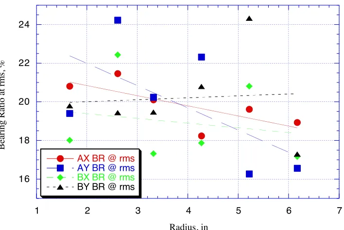
Bearing Ratio The bearing ratios measured at a distance of one RMS above the mean line ranged between 16% and 24%. Figure 1.15 is a plot of bearing ratio taken for each specimen in each direction at a height of 0.622 µm above the mean line. These values tend to remain

fairly constant with radius.

16 18 20 22 24

1 2 3 4 5 6 7

AX BR @ rms

AY BR @ rms

BX BR @ rms

BY BR @ rms

Bearing Ratio at rms, %

Radius, in

Figure 1.15 Bearing Ratio at one RMS from the mean surface

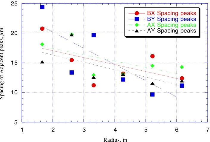
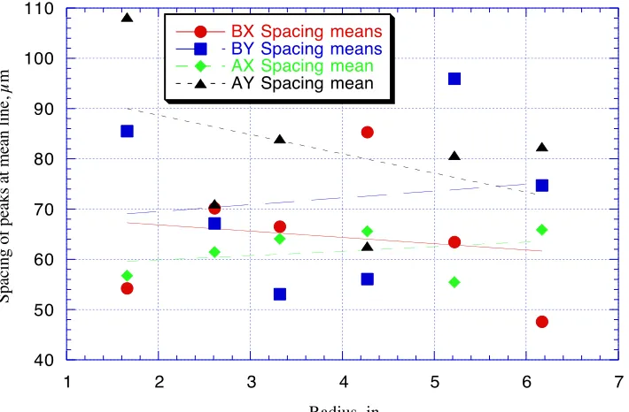
Peak Spacing The final measurement of the distribution of peaks and valleys for the textured surface is the spacing of the peaks. This illustrates the horizontal separation of the peaks rather than their heights. Figure 1.16 shows the spacing of the adjacent peaks independent of their size. The values began around 20 µm and decreased to around 12 µm. These measurements are smaller than the data in Figure 1.17 because it is a measure of all the adjacent peaks. Figure 1.17 shows the average spacing of the major peaks; that is, those peaks that pass through the mean line. The mean spacing between adjacent local peaks was much smaller and tended to decrease with radius. Figure 1.17 shows only the adjacent peaks where the valley between peaks is low enough to pass through the mean line. The mean spacing between peaks that crossed the mean was relatively constant with radius with an average of about 75 µm.

5 10 15 20 25

1 2 3 4 5 6 7

BX Spacing peaks

BY Spacing peaks

AX Spacing peaks

AY Spacing peaks

Spacing of Adjacent peaks, µm

40 50 60 70 80 90 100 110

1 2 3 4 5 6 7

BX Spacing means

BY Spacing means

AX Spacing mean

AY Spacing mean

Spacing of peaks at mean line, µm

Radius, in

Figure 1.17 Average spacing of the more significant peaks that pass through the mean line

the radius increased. Based on the measurements, the texturing produces nearly random grooves on the surfaces with a mean contact area of 4%.

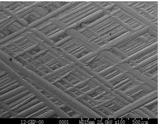
1.3.3 Scanning Electron Microscope

Micrographs of the textured surfaces were made using a scanning electron microscope in the backscatter mode. This mode provides more contrast for the atomic mass of the chemical species in the field of view because the efficiency of the back-scattered electron emission is dependent on atomic mass. The diamond grains (carbon) are more easily distinguished from the background (tin) surface. This enhanced contrast is also known as compositional or z-contrast.

Figure 1.18 100x image of the textured surface showing the overall features

areas charged with diamonds. Figure 1.19 is a 10x magnification of the center of Figure 1.18 showing several plateaus.

Figure 1.19 1000x image of the surface showing plateau between grooves

Figure 1.20 3000x image of the plateau showing individual diamonds (size 0.3-0.5 µm)

1.4 Current Lap Fabrication Process Problems

The process described was investigated for improvements in fabrication time and charging quality. One improvement deals with the preparation time of the lap. The time needed to fabricate a single plate can be 2 hours or more. New charging methods and equipment embed more diamond per unit time, thus reducing the overall fabrication time.

The reduction of the quantity of diamond used in the charging process was also investigated. Only a small percentage of the actual diamond in the slurry ended up embedded into the tin plate. Approximately 0.35% by volume of the slurry applied during charging is 0.25 µm

diamond. Using the averaged 4% contact area, the total charged area of the 35.5 cm diameter plate is 0.00396 m2. Therefore, the percentage of charged area to diamond area is 0.028%.

A third area concentrates on the predictability of the performance of the lapping plate after fabrication. It is rarely known how the plate will perform before leaving the production area. Studying the properties of the lapping plate as it was being fabricated helped determine a hypothesis for use in testing the charging quality.

2 N

P

T

P

2.0 Spiral Groove

A surface with a deterministic pattern of peaks and valleys than the textured plate was

studied in the form of a spiral groove. This pattern can be produced rapidly using a lathe and

the spacing and depth of the grooves can be changed easily. The geometry of the groove and

the plateau geometry can be changed by using different size, shape and quality tools such as

single crystal or polycrystalline diamond tools.

2.1 Grooving Parameters

The key parameters of the groove geometry are the pitch of the grooves, the width of the

land, the depth of the groove (or the height of the land), and the shape of the groove. The

first steps in the fabrication of the lap plates are similar to the previous process. The

machining was done on a Nanoform 600 Diamond Turning Machine (DTM). The high

purity tin plate described in Chapter 1, Section 1.1, was first rough faced using a

polycrystalline diamond tool with a nose radius of 1.2 mm. This is done to rid the surface of

diamonds from the previous fabrication and to get the entire surface of the plate consistently

flat. This facing cut was done at a feed rate of 20 mm/min and a depth of roughly 30 µm

with the plate rotating at 500 RPM. Once the polycrystalline tool has faced the plate, a final

pass is made using a large radius single crystal diamond tool. This pass was done at a slower

A spiral groove was then cut into the surface using the desired radius single crystal diamond

tool. The geometry of the tool and the depth of cut set the width of the groove, and the

feedrate and rotational speed of the plate determines the width of the lands. The feedrate

needed to produce the desired geometry can be determined using Equations 2.1 and 2.2.

L B

B= _o + (2.1)

2 4 8Rd d

B_o = − (2.2)

Here Bis the overall pitch [m], B_o is the width of the groove [m], L is the width of the land

[m], d is the depth of the groove [m] and R is the radius of the cutting tool [m] as seen in

Figure 2.1. The feedrate is then found by multiplying the overall pitch by the plate rotational

speed.

Figure 2.1 Definition of geometrical parameters of the grooved plate

The pitch of the grooves was based on the geometry of the heads being lapped on the plate.

The pitch of the grooves was set to ≈ 100 µm. This allows for a minimum of 10 grooves and

lands under each 1 mm wide head at one time. This will help to create a better quality lap

due to the small size of the features. Specimens from a plate fabricated using the spiral

groove geometry were measured in much the same way as the textured surface discussed in

the first part of this report. The tops of the lands are distorted during the grooving procedure +

B Bo L

as a result of the deformation of the soft tin by the diamond tool, as seen in Figure 2.2. This

effect is small in this case (< 0.5 µm) using a single crystal diamond tool. The deformation is

smaller for a single crystal tool than if a polycrystalline tool were used. A single crystal tool

has sharper cutting edges that a polycrystalline tool, thus the cutting forces are lower and less

of a plowing effect occurs. The pitch of the grooves in Figures 2.2 and 2.3 is 90 µm and the

ratio of land to groove is 47% (42µm land and 48 µm groove).

Figure 2.2 Talysurf of grooved plate after grooving

Figure 2.3 shows the surface after charging with the alumina ring. The distorted lands have

been flattened to less than 100 nm. A trace of the top of one of the lands showed a RMS

roughness of 22 nm and a Peak-to-Peak value of 80 nm. Note the relatively deep scratch on

top of one of the lands in Figure 2.3. The SEM pictures described next show this same

phenomenon.

Figure 2.3 Talysurf of grooved plate after charging

SEM Micrographs

The surfaces of the grooved plate were evaluated in the SEM to see if the charging process

produced a diamond concentration similar to the textured plate. The backscatter mode was

used to enhance the contrast between the diamond particles and the tin substrate.

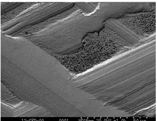
Figure 2.4 100x SEM images of grooved tin lap plate before charging (left) and after charging (right)

Figure 2.4 shows the surfaces at 100x with the machined surface at the left and the charged

surface at the right. Comparing this deterministic process to the random texturing process in

Figure 1.18 provides a striking contrast. But this comparison also shows much larger area of

contact for the particular groove-land geometry selected for this first test. The area of contact

is on the order of 50% in Figure 2.4 compared to a tenth of this value for the textured surface

shown in Figure 1.18.

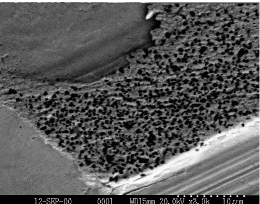
Figure 2.5 1000x SEM images of grooved plate before charging (left) and after charging (right)

The higher magnification images in Figure 2.5 illustrate the change in the flatness of the land

as a result of the charging process. Note that on the uncharged land at the left, lines parallel

to the grooves left by the tools during the machining process are visible, as are the raised

edges from cutting the groove. The charged land on the right is a much flatter surface and

reveals a series of scratches from the charging process. Also note in this picture what

appears to be a series of defects or inclusions that may be pulling out of the surface and

causing the visible scratches.

The highest magnification pictures in Figure 2.6 show an uncharged surface on the left

characterized by features in the machining direction and a charged surface at right

characterized by a uniform array of diamonds embedded in the tin surface. The scale marker

(small dots on the lower right of the image) is spaced at 1 µm indicating the diamond size is

the size of the diamonds in the slurry. The quantity of the diamonds in this region looks less

dense than the textured surface in Figure 1.20.

2.1.1 Film Thickness Model

To get an idea of how the grooving parameters affect the forces generated during lapping, a

film thickness model was developed to estimate both lift and drag forces during lapping. The

motion of the rows of heads over the surface of the plate will cause the glycol/water solution

used in the lapping procedure to be pulled along with them. As this fluid encounters the

features on the top of the lap surface it can generate a hydrodynamic film that will tend to

contact between the heads and the lap will be reduced and the lapping process will be

ineffective.

Figure 2.7 Sketch of head moving over the lap surface showing the velocity components

The spiral groove lap surface can be characterized by a series of grooves and lands, with

different spacing and directions depending on the fabrication technique. Generally, the

surface can be characterized as in Figure 2.7. The velocity of the heads (or rows of heads)

over the lap surface can be divided into components perpendicular and parallel to the

grooves.

The greatest hydrodynamic forces occur for motion perpendicular to the grooves. To

calculate the estimated hydrodynamic forces, the actual geometry of grooved plate illustrated

in Figure 2.1 was modeled both as a series of simple step bearings and a series of triangular

Figure 2.8 Pressure distribution and definition of the parameters pertinent to the hydrodynamic force generation of a step bearing

As illustrated in Figure 2.8, the peak pressure of a step bearing, P_PSB, per unit length L(into

the page) occurs at the front edge of the land and can be written as [4]

(

)

0 3

0 3 6

B B

h B

d h

Ud

P_PSB

− + +

= γ (2.3)

γ is the viscosity of the lubricant [Pa sec], U is the velocity component perpendicular to the

step [m/s], h is the film thickness [m], d is the depth of the groove [m], _B is the pitch of

the step [m], and B_o is the width of the groove [m]. Pitch, B Groove, Bo PP

B Bo

The vertical force of the step bearing,F_vSB , generated by one step as the head sweeps across

can be calculated by integrating the pressure distribution to produce the following

expression. BL P F PSB vSB 2 = (2.4)

Lis the overall length of the bearing into the page. One of the parameters of interest is the

proportion of the pitch allocated to land and to groove. The land ratio, LR, can be defined as

the ratio of the land to pitch. Combining Equation 2.3 and 2.4, the vertical force can be

written as

(

)

Here, W is the width of the slider across the grooves and all other terms are as previously

defined.

A triangular bearing was also modeled using a wedge bearing to help estimate the forces of

the rounded groove. While the triangular bearing has no actual land area, it helps to quantify

the forces of the extreme from the step bearing. The model is uses equations developed for

Figure 2.9 Wedge bearing geometry

Equation 2.6 is the lift of a bearing shown in Figure 2.9.

(

)

(

)

d d h d h d h ULB F_vTri +     ₋       + + = 2 2 ln 2 2 3 2 2 γ (2.6)

The geometry in Figure 2.9 can be converted into a continuous geometry as shown in Figure

2.10. Any geometry with a convergent shape can be used with the following model. The

analytical study of various configurations shows the shape itself has a rather small influence

on the load carrying capacity [4]. The forces generated by geometries like the ones shown by

Figure 2.10 Approximate pressure distribution of triangular bearings (solid line) and slight variance geometries

The pressure distribution for the triangular geometry is illustrated in Figure 2.10. The lift

and drag forces are ignored from B0 → B as the force at this region does not contribute

significantly to the total force. It is important to note that there is no land ratio for this type

of geometry. All that can be varied is the depth and width of the grooves. To get the total

lift, the vertical force generated per bearing of pitch B 2 in equation 2.6 is multiplied by the

number of bearings encountered, W B, as shown in Equation 2.6.

(

)

(

)

d d h d h d h UWLB F_vTri +     ₋       + + = 2 2 ln 2 6 2 3 2 γ (2.6) PP

B0 B

γ is the viscosity of the lubricant [Pa sec], U is the velocity component perpendicular to the

step [m/s], Lis the overall length of the bearing into the page [m], W is the width of the

slider across the grooves [m], h is the film thickness [m], B is the pitch of the step [m] and

d is the depth of the groove [m].

To study the estimated lift forces that would be generated during lapping, the following

values were used to find the force generated on an area equivalent to 24 strips of heads each

1.2 mm wide by 47 mm long moving perpendicular to the grooves. This would help to

establish a geometry that would not create forces that could interfere with the lapping

process.

γ = 0.021 Pa sec (ethylene glycol at room temperature)

U = 0.111 m_{/s (maximum speed of current kiss lapping)}

h = 0.125 µm (film thickness equivalent to _ max diamond size)

d = 10 µm or variable (groove depth)

B = 100 µm or variable (pitch of grooves)

o

B = 50 µm or variable (land ratio = 0.5)

Estimated Lapping Lift Forces

Using land ratio, groove depth and groove spacing as variables, the effect of the geometry of

each on the forces encountered during lapping can be estimated. During lapping, the heads

are pressed onto the lapping plate with a pressure of 49 kPa, or a force of 66.4 N. It is

important to keep the lift forces of the moving heads much lower than this as to not interfere

with the lapping process.

Variable Land Ratio Setting the groove depth and spacing to the specified values, the

generated lifting forces can be plotted versus the land ratio of a grooved plate, as shown in

Figure 2.11. Reducing the relative area of the land will increase the hydrodynamic film

pressure and the lift force during lapping.

Figure 2.11 Estimated hydrodynamic lift force versus land ratio for a grooved plate

0.0 5.0 10.0 15.0 20.0 25.0

0 0.1 0.2 0.3 0.4 0.5 0.6 0.7 0.8 0.9 1 Land Ratio

Vertical Force (N)

Step Triangular

Fixed: Groove Depth

Figure 2.11 shows the effect of changing the land ratio in Equation 2.5 from approximately 0

(99.9% groove) to 1 (all land). Note that the triangular groove lift force remains constant

since it is not a function of land ratio. It is safe to assume if the preload on the heads is larger

than 11 N, the hydrodynamic forces will be overcome by the preload (currently 66.4 N) and

contact will occur. It is important to note that as LR→0of the step bearing, Fv →0 as the

surface will no longer be a grooved surface but a plane.

Variable Groove Depth Setting the land ratio equal to 0.5, the groove depth can be varied

to see the effect of depth over a reasonable range. Figure 2.12 is a plot of the step bearing

and triangular bearing lift forces versus groove depth.

Figure 2.12 Estimated hydrodynamic lift force versus groove depth for a grooved plate

0.0 50.0 100.0 150.0 200.0 250.0 300.0 350.0 400.0 450.0 500.0

0 1 2 3 4 5 6 7 8 9 10

Groove Depth (um)

Vertical Force (N)

Step Triangular

Fixed: Land Ratio

The bearings follow the same trend with respect to a changing groove depth. As the depth of

the groove gets smaller than 6 µm in the step bearing model, the forces become significant

and can overcome the preload reducing the contact between lap and heads. This does not

happen with the triangular bearings because of the lack of a sharp discontinuity in the

geometry. As the depth of the groove gets smaller with the triangular bearing the surface

profile approaches a plane. When the groove depth equals 0, the total lift force is zero since

the surface is actually a plane.

Variable Groove Pitch If the groove spacing (or pitch) is reduced holding everything else

constant, the vertical force will be reduced as shown in Figure 2.13. The reason for this

effect is that if the length of the bearing is subdivided into short step bearings, each will

generate a smaller peak pressure and if added together will generate less lift than if the whole

Figure 2.13 Estimated hydrodynamic lift force versus groove pitch for a grooved plate

The triangular bearings produce a larger overall lift force as compared to the step bearing.

This is due to higher overall pressures generated with the triangular bearings. It’s safe to

assume that the lift forces generated by the actual plate profile, illustrated in Figure 2.1, lies

between the estimated forces shown in Figures 2.11 through 2.13.

0.0 5.0 10.0 15.0 20.0 25.0

0 20 40 60 80 100 120

Groove Pitch (um)

Vertical Force (N)

Step Triangular

Fixed: Land Ratio

Estimated Lapping Drag Forces

The drag force on the rows of heads from the shear of the lubricant film can be estimated in

much the same way as for the vertical force. An expression for the step bearing using the

same parameters from Equations 2.3 through 2.5 is [4]

(

)

(

(

)

)

F_DSB 1

) 1 ( 3 3 3 2 γ (2.7)

An expression for the drag forces from the triangular bearings using the same parameters as

equation 2.6 is [4]

(

)

(

)

The same evaluation of the parameters of interest can be performed as in the vertical force

Variable Land Ratio Figure 2.14 show the influence of land ratio on the drag force. The

drag force for the step bearing is linearly proportional to the land ratio with the smallest value

when the land is small compared to the groove width, or LR << 1.0. As the land grows, so

does the drag. However the drag force for the triangular groove remains constant since it is

not a function of land ratio.

Figure 2.14 Estimated hydrodynamic drag force versus land ratio for a grooved plate

0.0 5.0 10.0 15.0 20.0 25.0 30.0

0 0.1 0.2 0.3 0.4 0.5 0.6 0.7 0.8 0.9 1 Land Ratio

Drag Force (N)

Step Triangular

Fixed: Groove Depth

Variable Groove Depth The effect of changing the depth of the groove on the drag force is

shown in Figure 2.15. In this case the drag force grows as the depth of the groove is reduced,

much like the lift force shown in Figure 2.12. If the groove depth is kept 10 µm or larger, the

drag force will be relatively small.

Figure 2.15 Estimated hydrodynamic drag force versus groove depth for a grooved plate

Variable Groove Pitch The last parameter to be discussed is the spacing, or pitch, of the

grooves shown in Figure 2.16. For the lift in Figure 2.13, the effect of reducing the pitch was

to reduce the vertical force generated in the bearing. However, changing the pitch has no

effect on the drag force. The result is the same if a single step is used or if the length is

subdivided into a number of shorter step bearings. The reason is that it is the land ratio that

determines the drag, and in both of these cases half of the bearing is a land and half is a

groove.

0.0 2.0 4.0 6.0 8.0 10.0 12.0 14.0 16.0 18.0 20.0

0.0 2.0 4.0 6.0 8.0 10.0 12.0 14.0 16.0 18.0 20.0 Groove Depth

Drag Force (N)

Step Triangular

Fixed: Land Ratio

Figure 2.16 Estimated hydrodynamic drag force versus groove pitch for a grooved plate

The triangular bearing produces a much smaller overall drag force than that of the step

bearing. This is due to the continuous geometry of the bearing, as opposed to the sharp

discontinuity experienced with the step bearing. The fluid flow model of the diamond slurry

in the grooves during lapping showed the key parameters to be: 1) depth of groove, 2) width

of groove, and 3) width of flat land between grooves.

Reviewing Figures 2.11 through 2.16, to keep lift forces minimal, the land ratio should be

large, the groove depth ≥ 10 µm, and the groove pitch small. The keep the drag forces

minimal during lapping, the land ratio should be small, the groove depth ≥ 10.0 µm and the

groove pitch does not affect the drag forces. Drag forces are more of a concern than the

lifting forces. The lapping fixture applies a 66.4 N preload onto the lapping plate. Thus if

0.0 2.0 4.0 6.0 8.0 10.0 12.0 14.0

0.0 20.0 40.0 60.0 80.0 100.0 120.0

Groove Pitch (um)

Drag Force (N)

Step Triangular

Fixed: Land Ratio

the lift forces are kept well below 60 N, the lapping quality should not be altered at all.

However, the drag force may cause the AlTiC pieces to be pushed off the pad. Since they are

attached to the lapping fixture by a sticky surface on the foam pad, if the drag forces were too

high, they may simply be pushed off. Studying the magnitude of the predicted forces in both

lift and drag force models, the groove geometry was decided to be land ratio = 0.25 – 0.30,

groove depth = 10.0 µm. Using a 40 µm radius tool, the pitch for a land ratio was calculated

to be 80.0 µm. This would produce a lift force between 5.5 N (step model) and 18.0 N

(triangular model), much lower than the 66.4 N preload. The drag forces due to the fluid

would be between 1.8 N (triangular model) and 7.2 N (step model). The effects of these

forces will be discussed later in Chapter 5, Section 5.4.

2.1.2 Groove Tool Geometry Effects On Machining

To study the groove geometry produced by different tool shapes, a round nosed cutting tool

and a dead sharp cutting tool were each used to groove a plate. A difference in the

machining properties of the tin was observed after the use of the two tools.

The dead sharp tool has 2 flat sides 60° apart that meet at a

sharp tip (dashed line in Figure 2.17). The round nosed tool

has a 40 µm radius tip with a 60° window (solid line in

60°

40 µm

Figure 2.17). Due to the difference in tool geometry, a common feature of the groove had to

be set. The groove width was selected and set to 50 µm for both tools. This set the depth of

the dead sharp tool to 43.3 µm and the round nosed tool to 7.8 µm.

Dead Sharp Tool

Grooving the plate with the dead sharp tool produced an unexpected result; a macroscopic

granular appearance was plainly visible to the naked eye. The “grains” had a diameter

varying from 5 mm to 0.5 mm as shown in the photograph in Figure 2.18.

Figure 2.18 Tin plate surface grooved with dead sharp tool

The appearance of these “grains” caused much speculation as to their origin as well as their

effect on the charging and lapping process. Are they really grains? Should they be that big?

Why are they visible only after the plate is grooved? To understand the origin of these

granular features, SEM micrographs of the individual grain boundaries were studied to see

why the features were visible. Figure 2.19 illustrates the edge of one grain and helps explain

to grain. In the grain on the left, the peaks of the grooves are sharp: on the right, the peaks

have large burrs attached that shade the bottom of the grooves and modify their reflectivity.

Figure 2.19 SEM imaging of tin surface features created by dead sharp tool at 200x (left) and 600x (right)

Metallographic analysis of the rolled tin indicates that the material does, in fact, have large

grains on the order of 1-2 mm. In metal grains, there can be a difference in the plastic strain

response depending on the orientation of the individual grain [5]. Such a variation could

make each grain respond differently to the cutting forces and thereby produce the features

seen in Figure 2.18. The fact that this variation is so pronounced in tin depends on several

factors. Tin is a low melting temperature material and the homologous temperature, or the

temperature divided by the melting temperature, is 0.59 at room temperature. Consequently,

tin will undergo "hot deformation" at room temperature and will be quite soft and ductile.

shows an illustration of the tetragonal and cubic crystal structures. A grain must be able to

undergo an arbitrary shape change for compatible plastic strain. Because the strain tensor is

symmetric and volume is constant, there must be five independent degrees of freedom in the

total plastic strain. Plastic strain due to slip is the linear superposition of the strain tensors for

all active slip systems, and each slip system has one free variable, the shear strain. This

means that you must have at least five linearly independent slip systems.

Figure 2.20 Tetragonal crystal structure (left) and cubic crystal structure (right)

In general, tetragonal crystal structures have significantly fewer slip systems available than

do the cubic crystal structures. Although the details are complicated by the fact that the

formation of burrs in machining is multi-axial, shearing-fracture process, one can expect that

in tin there will be grain orientations where the plastic straining process is constrained by a

lack of independent slip systems. This will lead to anisotropy in the burr formation process

depending on grain orientation as illustrated in Figure 2.21. Slip system constraints are

therefore considered to be a contributing factor for the results seen in Figures 2.18 and 2.19.

In comparison, the burr-formation anisotropy is expected to be less for cubic metals such as

copper or aluminum since these have a large number of equivalent slip systems available.

A

C B A

C B

Figure 2.21 Illustration of various burr sizes for varying grain orientations

Round Nosed Tool

The visible grainy appearance of the grooved plate was not as apparent when the plate was

machined with the round nose tool. Figure 2.22 shows a comparison the chip geometry for

each tool. The depth of cut is much smaller for the round nose tool to produce the same

groove width. As stated before, the test done with equal groove widths produced a dead

sharp tool depth of cut of 43.3 µm, versus a 7.8 µm depth of cut with the round nosed tool.

Since less material must be removed, the forces are smaller, and the plowing effect is

reduced. The net effect is that the burr formation that dominates the appearance when using

the dead sharp tool is not a major factor when using the round nosed tool.

Since the dead sharp tool exaggerated burr formation, it was decided a round nosed tool

would be best for grooving. Another advantage of the round nosed tool is that the grooves

can remain shallow and wide, whereas with the dead sharp tool, a deeper groove is needed

for an equivalent width. This additional depth is unnecessary since the fluid force model

determined that fluid flow effects are roughly equivalent at depths of 10µm or more.

While exaggerated burr formation is not a major problem when grooving with a round nose

tool, the raised edges of the lands were still a problem. The procedure for grooving the plate

was to face it with a large nose radius tool (0.5 mm) and then cut the grooves with the 40 µm

nose radius tool. The final pass made with the single crystal tool in the facing cut produced a

flat mirror-like surface on the tin. As described in Section 2.1 and shown in Figure 2.2, when

the round nose tool was used to groove the plate, the tool tended to make a burr, making the

land have raised edges. These edges are reported to affect the charging process, as the lands

will not charge where these are present. This is because initially the raised edges are the only

areas of contact between the plate and the charging ring, and thus the lands are not fully

charged until the edges flatten to the level of the lands. One solution to ridding of these is to

do a shallow pass over the plate on the DTM after the grooving pass and cut the tops of the

lands off. Another possibility is to increase the stress during the charging process to yield the