Online Performance Anomaly Prediction and Prevention for Complex Distributed Systems.

(1)

ABSTRACT

TAN, YONGMIN. Online Performance Anomaly Prediction and Prevention for Complexdummy

Distributed Systems. (Under the direction of Dr. Xiaohui (Helen) Gu.)

Real world distributed systems (e.g., cloud computing infrastructures, enterprise data cen-ters, massive data processing systems) have become increasingly complex as they grow in both scale and functionality. However, such complexity makes these systems vulnerable to perfor-mance anomalies caused by various faults such as resource contentions, perforperfor-mance bottlenecks, software bugs, and hardware failures. It is a daunting task for system administrators to manu-ally keep track of the execution status of many distributed hosts all the time in order to search anomaly root causes and correct performance anomalies. Therefore, it is imperative to develop automated system anomaly management schemes to achieve robust distributed systems with a minimum requirement for human intervention.

This dissertation focuses on exploring the key techniques for building robust distributed systems. It includes three studies on system performance anomaly prediction and one study on scalable and resilient system monitoring. The following are the key contributions of this dissertation:

First, we present a set of online anomaly prediction models that aim at raising advance alerts prior to anomaly occurrences so that they can provide a window of opportunity (i.e., lead time) for predictive anomaly prevention and alleviation. We propose integrated prediction models that combine the attribute value prediction (Markov chain model) and the statistical classification methods (naive Bayesian classifier and tree-augmented Bayesian networks). We also propose a decision tree based prediction model that introduces an additional alert state other than normal and anomaly states to achieve advance anomaly prediction. We further present comprehensive measurement studies to quantify the predictability of different real-world system performance anomalies. We observe that those real system anomalies do exhibit predictability and our anomaly prediction models can achieve high prediction accuracy with generous lead time and low prediction overhead.

(2)

high prediction accuracy.

Third, a complete solution of predictive system performance anomaly management requires not only accurate anomaly prediction models but also anomaly prevention to steer the system away from the potential abnormal state. To this end, we present a novel predictive performance anomaly prevention system that integrates online anomaly prediction and virtualization-based prevention techniques. Our system can raise advance anomaly alerts and perform coarse-grained anomaly cause inference to pinpoint the faulty application components and infer the most relat-ed system metrics. Basrelat-ed on those prrelat-ediction results, our system uses virtualization techniques to perform virtual machine perturbations (e.g. elastic resource scaling, live virtual machine migration) to prevent the impending performance anomalies.

(3)

(4)

Online Performance Anomaly Prediction and Prevention for Complex Distributed Systems

by Yongmin Tan

A dissertation submitted to the Graduate Faculty of North Carolina State University

in partial fulﬁllment of the requirements for the Degree of

Doctor of Philosophy

Computer Science

Raleigh, North Carolina 2012

APPROVED BY:

Dr. Frank Mueller Dr. Xiaosong Ma

Dr. William Enck Dr. Hui Lei

(5)

DEDICATION

(6)

BIOGRAPHY

(7)

ACKNOWLEDGEMENTS

Pursing a PhD degree is a long journey with both bitter and sweet memories. I would not have reached the ﬁnish line without the support and inspiration of many people. At all stages of my graduate study, I have received numerous kindly help from them, whom I undoubtedly owe gratitude to. Therefore, the acknowledgements make an indispensable part of this dissertation. First, I would like to express my deep gratitude to my advisor, Dr. Xiaohui Gu, for her expert guidance, consistent encouragement, and patience to shepherd me throughout my PhD pursuit. Her knowledge and experiences on research, insightful thoughts and suggestions have been of exceptional value to me. I also want to thank Dr. Frank Mueller, Dr. Xiaosong Ma, Dr. William Enck, and Dr. Hui Lei for their time and eﬀorts serving on my advisory committee and providing valuable advice that helped to improve this dissertation.

Second, I would like to thank all the former or current members in DANCE group for their friendship and the fun time spent together in the lab: Zhenhuan Gong, Junjie Ni, Juan Du, Prakash Ramaswamy, Raghukishor Kandula, Vinay Venkatesh, Sethuraman Subbiah, Kamal Kc, Hiep Nguyen, Zhiming Shen, Daniel Dean, Chin-Jung Hsu and Anson Ho.

Third, I want to thank the friends I have met with at NC State. Just to name a few: Xing Wu, Feng Ji, Fei Meng, Zhengzhang Chen, Yaogong Wang, Yingying Wang and Siqi Xu for their warm-hearted helps in research, courses, and in daily life. I also want to thank all the buddies of Chinese Student Soccer Club. Weekly soccer practices always replenish me with more strength and energy for my work.

Fourth, I would like to thank the staff of Office of International Students, Department of Computer Science, and Graduate School Office at NC State and to everyone else behind the scenes for all their help. Because of them, my graduate study has been smooth without worrying about too many stuffs besides academics. I am also grateful to organizations that generously funded my graduate research. The work in this dissertation is supported in part by US National Science Foundation (NSF) and the US Army Research Office (ARO) under several grants. As usual, any opinions expressed in this dissertation are those of the author and do not necessarily reflect the views of NSF, ARO, or U.S. Government.

(8)

TABLE OF CONTENTS

List of Tables . . . vii

List of Figures . . . .viii

Chapter 1 Introduction . . . 1

1.1 Motivation . . . 2

1.2 Summary of the State of the Art . . . 2

1.3 Thesis Statement . . . 3

1.4 Research Challenges . . . 4

1.5 Summary of Contributions . . . 5

1.6 Assumptions . . . 6

1.7 Organization of Dissertation . . . 6

Chapter 2 Problem Overview . . . 8

2.1 System Performance Anomaly Prediction and Prevention . . . 8

2.2 Scalable System Monitoring . . . 10

Chapter 3 Online Anomaly Prediction Models and Case Studies . . . 13

3.1 Preliminary . . . 13

3.2 Bayesian Classiﬁer Based Anomaly Prediction Model . . . 14

3.2.1 Approach Overview . . . 14

3.2.2 Design Details . . . 15

3.3 Decision Tree Based Anomaly Prediction Model . . . 20

3.3.2 Design Details . . . 20

3.4 Implementation and Evaluation . . . 22

3.4.1 Anomaly Data Collection . . . 22

3.4.2 Evaluation Metrics . . . 24

3.4.3 Results and Analysis . . . 25

3.5 Summary . . . 36

Chapter 4 Adaptive System Anomaly Prediction Using Self-Evolving Models 37 4.1 System Design . . . 38

4.1.2 Dynamic Computing Context Discovery . . . 39

4.1.3 Adaptive Runtime Anomaly Prediction . . . 42

4.2.1 System Implementation . . . 43

4.2.2 Experiment Setup . . . 44

(9)

Chapter 5 Predictive Performance Anomaly Prevention for Virtualized Cloud

Systems . . . 53

5.1 System Design . . . 54

5.1.2 Per-VM Anomaly Prediction Model . . . 56

5.1.3 Online Anomaly Cause Inference . . . 57

5.1.4 Predictive Prevention Actuation . . . 58

5.2.1 Experiment Setup . . . 60

5.3 Summary . . . 67

Chapter 6 Resilient Self-Compressive Monitoring for Large-Scale Hosting In-frastructures . . . 69

6.1 Preliminary . . . 70

6.1.1 Monitoring System Model . . . 70

6.1.2 Problem Formulation . . . 71

6.2 System Design . . . 72

6.2.1 Overview . . . 73

6.2.2 Online Reference Block Search . . . 74

6.2.3 Failure Resilience . . . 77

6.2.4 Analytical Study . . . 78

6.3.1 System Implementation . . . 84

6.3.2 Trace Data Collection and Statistics . . . 85

6.4 Summary . . . 97

Chapter 7 Related Work . . . 98

7.1 Online System Anomaly Management . . . 98

7.2 Distributed System Monitoring . . . 101

Chapter 8 Conclusion and Future Work . . . .104

8.1 Contributions . . . 104

8.2 Future Work . . . 106

(10)

LIST OF TABLES

Table 3.1 Subset of monitored attributes. . . 22

Table 3.2 Anomaly prediction system overhead comparisons. . . 35

Table 3.3 Overhead comparisons between the basic Markov model and the two-dependent Markov model. . . 35

Table 5.1 PREPARE System overhead measurements. . . 67

Table 6.1 Notations. . . 70

Table 6.2 Statistics of the monitoring traces. . . 85

Table 6.3 Sensitivity study summarization of all the intra-node attribute datasets. . 94

Table 6.4 Sensitivity study summarization of all the inter-node attribute datasets. . . 95

Table 6.5 System overhead comparison for compressing an intra-node Google cluster CPU usage trace containing 1296 hosts. . . 96

(11)

LIST OF FIGURES

Figure 1.1 Infrastructure-as-a-Service (IaaS) cloud architecture. . . 1

Figure 2.1 The diﬀerence between anomaly prediction and anomaly detection. . . 9

Figure 2.2 Distributed monitoring system. . . 10

Figure 2.3 A case study for ﬁne-grained monitoring. . . 11

Figure 2.4 Scalability bottleneck at the management node. . . 11

Figure 3.1 Bayesian classiﬁer based anomaly prediction model. . . 14

Figure 3.2 The state transition diagram of the Markov chain model for an attribute. This attribute ranges from 0 to 30. We discretize the attribute values into three states. Each directed arc is labeled with the corresponding state transition probability. . . 15

Figure 3.3 Two-dependent Markov model for attribute value prediction. . . 17

Figure 3.4 Naive Bayesian classiﬁer. . . 18

Figure 3.5 TAN classiﬁer. . . 18

Figure 3.6 Tunable anomaly predictor with diﬀerent alert intervals. . . 20

Figure 3.7 Anomaly prediction using a decision tree classiﬁer. . . 21

Figure 3.8 Markov prediction error for PlanetLab data: quantization scheme. . . 26

Figure 3.9 Markov prediction error for PlanetLab data: quantization granularity. . . 26

Figure 3.10 Classiﬁcation ROC curves for PlanetLab data: naive Bayesian. . . 27

Figure 3.11 Classiﬁcation ROC curves for PlanetLab data: TAN. . . 27

Figure 3.12 Advance anomaly prediction accuracy for PlanetLab data: naive Bayesian + Markov. . . 28

Figure 3.13 Advance anomaly prediction accuracy for PlanetLab data: TAN + Markov. 28 Figure 3.14 Advance anomaly prediction accuracy for PlanetLab data: decision tree classiﬁer. . . 28

Figure 3.15 Markov prediction error for SMART data: quantization scheme. . . 29

Figure 3.16 Markov prediction error for SMART data: quantization granularity. . . 29

Figure 3.17 Classiﬁcation ROC curves for SMART data: naive Bayesian. . . 30

Figure 3.18 Classiﬁcation ROC curves for SMART data: TAN. . . 30

Figure 3.19 Advance anomaly prediction accuracy for SMART data: naive Bayesian + Markov. . . 30

Figure 3.20 Advance anomaly prediction accuracy for SMART data: TAN + Markov. 30 Figure 3.21 Markov prediction error for System S data: quantization scheme. . . 31

Figure 3.22 Markov prediction error for System S data: quantization granularity. . . . 31

Figure 3.23 Classiﬁcation ROC curves for System S data: naive Bayesian. . . 32

Figure 3.24 Classiﬁcation ROC curves for System S data: TAN. . . 32

Figure 3.25 Advance anomaly prediction accuracy for System S data: naive Bayesian + Markov. . . 32

(12)

Figure 3.28 Prediction lead time for System S data: TAN + Markov. . . 33

Figure 3.29 Prediction lead time for System S data: decision tree classiﬁer. . . 33

Figure 3.30 Anomaly prediction accuracy comparison between (two-dependent Markov model + TAN model) and (basic Markov model + TAN model). . . 34

Figure 4.1 Context-aware anomaly prediction. . . 39

Figure 4.2 Number of execution contexts in dynamic systems. . . 45

Figure 4.3 True positive rate (AT) and false alarm rate (AF) for the IBM System S Join component with the memory leak fault: ProcTime Anomaly. . . 46

Figure 4.4 True positive rate (AT) and false alarm rate (AF) for the IBM System S Join component with the memory leak fault: Throughput Anomaly. . . . 46

Figure 4.5 True positive rate (AT) and false alarm rate (AF) for the IBM System S Join component with the loopErr fault: ProcTime Anomaly. . . 47

Figure 4.6 True positive rate (AT) and false alarm rate (AF) for the IBM System S Join component with the loopErr fault: Throughput Anomaly. . . 47

Figure 4.7 True positive rate (AT) and false alarm rate (AF) for the IBM System S Join component with the buﬀerErr fault: ProcTime Anomaly. . . 48

Figure 4.8 True positive rate (AT) and false alarm rate (AF) for the IBM System S Join component with the buﬀerErr fault: Throughput Anomaly. . . 48

Figure 4.9 True positive rate (AT) and false alarm rate (AF) for the IBM System S Diﬀuser component with the memory leak fault: ProcTime Anomaly. . . . 49

Figure 4.10 True positive rate (AT) and false alarm rate (AF) for the IBM System S Diﬀuser component with the memory leak fault: Throughput Anomaly. . 49

Figure 4.11 True positive rate (AT) and false alarm rate (AF) for Ping failure predic-tion accuracy on the PlanetLab: Average predicpredic-tion accuracy. . . 50

Figure 4.12 True positive rate (AT) and false alarm rate (AF) for Ping failure predic-tion accuracy on the PlanetLab: Predicpredic-tion accuracy on host A. . . 50

Figure 4.13 True positive rate (AT) and false alarm rate (AF) for Ping failure predic-tion accuracy on the PlanetLab: Predicpredic-tion accuracy on host B. . . 50

Figure 4.14 ALERT prediction lead time: System S. . . 51

Figure 4.15 ALERT prediction lead time: PlanetLab. . . 51

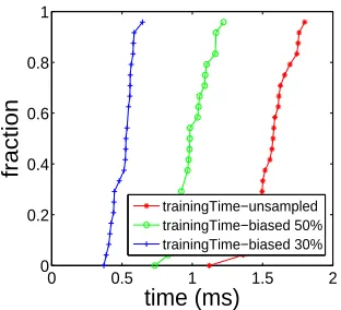
Figure 4.16 True positive rate (AT) and false alarm rate (AF) under diﬀerent sub-sampling rates: Join component: ProcTime Anomaly. . . 51

Figure 4.17 True positive rate (AT) and false alarm rate (AF) under diﬀerent sub-sampling rates: Ping Failure on host A. . . 51

Figure 4.18 ALERT system computation cost: Training time. . . 52

Figure 4.19 ALERT system computation cost: Prediction time. . . 52

Figure 5.1 Overall architecture of the PREPARE system. . . 54

Figure 5.2 Attribute selection using the TAN model. . . 57

Figure 5.3 The topology of the System S application. . . 59

Figure 5.4 The topology of the RUBiS application. . . 59

(13)

Figure 5.6 Sampled SLO metric trace comparison using the elastic VM resource

s-caling as the prevention action. . . 62

Figure 5.7 SLO violation time comparison using the live VM migration as the pre-vention action. . . 63

Figure 5.8 Sampled SLO metric trace comparison using the live VM migration as the prevention action. . . 64

Figure 5.9 Anomaly prediction accuracy comparison between the per-component model and the monolithic model. . . 65

Figure 5.10 Anomaly prediction accuracy comparison under diﬀerent settings of the false alarm ﬁltering for a bottleneck fault in RUBiS. . . 66

Figure 5.11 Anomaly prediction accuracy comparison under diﬀerent sampling inter-vals for a bottleneck fault in RUBiS. . . 66

Figure 6.1 System image of an inter-node attribute for a distributed system of N nodes. . . 72

Figure 6.2 System image of an intra-node attribute for a distributed system of N nodes. . . 72

Figure 6.3 RCM distributed monitoring architecture. . . 73

Figure 6.4 Online training phase. . . 74

Figure 6.5 RCM’s reference block search algorithm. . . 76

Figure 6.6 Compression ratio comparison for the VCL IP Statistics trace. . . 87

Figure 6.7 Compression ratio comparison for the VCL NT Processor trace. . . 87

Figure 6.8 Compression ratio comparison for the PlanetLab CPU load trace. . . 88

Figure 6.9 Compression ratio comparison for the PlanetLab free memory trace. . . . 89

Figure 6.10 Compression ratio comparison for the Google cluster CPU trace. . . 89

Figure 6.11 Compression ratio comparison for the Google cluster memory trace. . . . 90

Figure 6.12 Compression ratio comparison for the PlanetLab inter-node delay trace. . 90

Figure 6.13 Compression ratio comparison for the traﬃc matrices trace. . . 91

Figure 6.14 Compression ratio comparison for the Google cluster CPU trace under host failures. . . 91

Figure 6.15 Compression ratio comparison for the Google cluster memory trace under host failures. . . 92

Figure 6.16 Compression ratio comparison for the PlanetLab inter-node delay trace under host failures. . . 92

(14)

Chapter 1

Introduction

Large-scale hosting infrastructures such as Infrastructure-as-a-Service (IaaS) cloud systems [2] have become the fundamental platforms for many real world distributed systems and appli-cations (e.g., cloud computing systems [15], enterprise data centers, massive data processing systems [49], and web hosting services). Figure 1.1 shows a typical architecture of the IaaS cloud. Users can lease these computing resources in a pay-as-you-go fashion based on their actual de-mands. Since IaaS cloud systems are often shared by multiple users (i.e. multi-tenancy), cloud computing service providers usually leverage virtualization technologies to achieve isolation a-mong diﬀerent users. Therefore, multiple users can run their applications within the virtual machines (VMs) allocated to them to share a common physical computing infrastructure.

VM VM

VM VM VM VM VM VM VM VM

Phones

Desktops

Servers

Laptops

Infrastructure-as-a-Service Cloud

VM VM

VM

Normal applications

Abnormal applications

(15)

1.1 Motivation

Real-world distributed systems hosted by large-scale virtualized hosting infrastructures have become increasingly complex as they grow in both scale and functionality. Unfortunately, such complexity and the inherent sharing nature make these systems vulnerable to performance anomalies caused by various reasons such as resource contentions, performance bottlenecks, misconfigurations, software bugs and hardware failures. For example, Amazon Elastic Compute Cloud (EC2) recently experienced perhaps the worst service outage [13] in cloud computing’s history. The service outage was initially caused by an error in the network configuration pro-gram. It lasted more than 100 hours and affected thousands of EC2 customers in the whole US east region.

Therefore, one of the key concerns for complex distributed systems is system robustness, which measures the ability of a distributed system to continue to function correctly despite the existence of faults that may lead to performance anomalies. To achieve system robustness, we hope to detect and correct system performance problems in a timely manner. However, it is a challenging task for system administrators to manually keep track of the execution status of many distributed hosts all the time in order to ﬁnd out the most likely causes and correct the problems accordingly. Thus, it is imperative to provideautomated system anomaly management

to achieve robust distributed systems with the minimum requirement of human intervention. In addition,scalable system monitoring serves as one of the building blocks for system anomaly management schemes. It can provide complete and ﬁne-grained information about all hosts and network conditions within the distributed system to drive the decision making of the system anomaly management module.

1.2 Summary of the State of the Art

(16)

It is a difficult task to deploy fine-grained monitoring for large-scale hosting infrastruc-tures due to the scalability concern. Previous work has identified this scalability challenge and proposed various solutions: 1) employing decentralized architectures such as hierarchical aggre-gation [104] or peer-to-peer structure [79,111] to distribute monitoring workload, and 2) trading off information coverage [71] or precision [62] for lower monitoring cost. In addition, one promis-ing category of approaches perform online data compression to reduce the monitorpromis-ing traffic from the distributed worker nodes to the management node. For example, recent work [59, 114] has proposed to exploit temporal and/or spatial correlations for data compression. However, only exploring temporal correlation has limited compression power while discovering spatial correlation is often costly due to the expensive clustering operation [114].

1.3 Thesis Statement

The major focus of this dissertation is to understand the limitations of the existing system anomaly management schemes and to develop new techniques to improve the state of the art. More speciﬁcally, we hope to predict impending system anomalies in advance and take pre-ventive actions to mitigate the negative impact of potential anomalies. We limit the scope of anomalies to system performance anomalies, which means any unexpected performance degra-dations (e.g., service level objective violations).

We study the behavior of several real-world system performance anomalies. We observe that most of the system performance anomalies usually manifest as visible changes of various system-level metrics. For example, a performance anomaly caused by a memory leak fault might exhibit a downward change pattern for the “free memory” metric before it starts to aﬀect the system performance. If we can collect these metric samples with suﬃcient sampling granularity, we believe that capturing such pre-anomaly system behavior can provide us some lead time (i.e., a window of opportunity ahead of impending performance anomaly) for early anomaly prediction and prevention. Therefore, we make the following thesis statement.

Anomaly prediction techniques using ﬁne-grained data sampling intervals can eﬀective-ly improve distributed system robustness by raising advance alerts and taking preventive

actions before performance anomalies occur.

(17)

integrates anomaly prediction and anomaly prevention to achieve a complete automated anoma-ly management. Our ﬁnal study develops a compressive monitoring system that can provide ﬁne-grained information with low overhead. However, the compressive monitoring system is generic, which is not limited to support anomaly prediction and can be applied to any other system management functions.

1.4 Research Challenges

It is challenging to provide successful anomaly management schemes and scalable monitor-ing schemes for achievmonitor-ing robust distributed systems. We identify the followmonitor-ing key research challenges:

Black-box analysis: Applications running inside IaaS clouds often appear opaque to the service providers. It is difficult to apply previous white-box or grey-box approaches [19,30] that need modifications or instrumentation to the applications or their underlying sys-tems (e.g. middlewares). Therefore, we require a black-box, application-agnostic anomaly management model that does not need any prior knowledge about the hosted application. Online processing: Many tough bugs that cause system performance anomalies often on-ly manifest during large-scale runs. It is difficult for system administrators to reproduce production-run problems in house for offline diagnosis. Therefore, we require an online anomaly management model that can take first-aid actions to prevent performance anoma-lies occurred in production runs.

Advance prediction: If the anomaly management system can predict a potential perfor-mance anomaly in advance, it can apply countermeasures to prevent the occurrence of the predicted anomaly. However, predicting into the future is challenging in nature. In our scenario, prediction means the model should capture and analyze some pre-anomaly system behaviors (i.e., symptoms) in order to raise advance alerts.

(18)

the overhead will outweigh the beneﬁt of applying the automatic anomaly management scheme.

Scalable and resilient monitoring: It is a challenging task to deploy ﬁne-grained monitoring for large-scale hosting infrastructures due to the scalability concern. Furthermore, host failures are common in large-scale distributed systems. Therefore, we need a scalable and failure resilient monitoring solution that can collect ﬁne-grained monitoring data with low overhead and is robust to host and network failures.

In this dissertation, we will explore a set of system anomaly prediction and scalable mon-itoring solutions, which are essential for enhancing system robustness for complex distributed systems.

1.5 Summary of Contributions

The contributions of this dissertation are summarized as follows:

Online anomaly prediction models [96,97]: We first develop an integrated prediction mod-el that combines the attribute value prediction (Markov chain modmod-el) and the statistical classification methods (naive Bayesian classifier and tree-augmented Bayesian networks). We then present a decision tree classifier that introduces an additional alert state other than normal and anomaly states to achieve advance anomaly prediction. Both predic-tion models aim at raising advance alerts prior to impending performance anomalies so as to provide a window of opportunity (i.e., lead time) for predictive system recovery. We further present comprehensive measurement studies to quantify the predictability of different real-world system performance anomalies. We observe that real system anoma-lies do exhibit predictability and our online anomaly prediction model can achieve high prediction accuracy with generous lead time and low overhead.

Adaptive anomaly prediction model [97]: We extend our anomaly prediction models by making the models adaptive to dynamic execution environments. We first use a hier-archical clustering algorithm to discover different execution contexts. We maintain an ensemble of prediction models, one for each discovered execution context. During run-time, we dynamically switch between different prediction models according to context evolving patterns. We find that our context-aware model can achieve higher prediction accuracy than the monolithic model as well as the traditional ensemble model.

(19)

virtualization-based prevention techniques. Our system can raise advance anomaly alerts and perfor-m coarse-grained anoperfor-maly cause inference to pinpoint faulty coperfor-mponents and infer the anomaly causes. Based on the anomaly prediction and cause inference results, our system leverages virtualization techniques to perform virtual machine perturbations (e.g. elastic resource scaling [51, 91], live virtual machine migration [36]) as the countermeasures to prevent the impending performance anomalies.

Scalable and resilient distributed monitoring system [99, 100]: We develop a novel image-based monitoring system for large-scale hosting infrastructures. We address the scalability problem by applying online data compression on live monitoring data streams to reduce the distributed monitoring cost. We model snapshots of the distributed system as a se-quence of system images and apply lightweight online reference block search algorithms to compress distributed monitoring data. Our system is also failure resilient, which can tolerate host and network failures that are common in real-world hosting infrastructures.

1.6 Assumptions

Our work makes a set of assumptions that are summarized as follows.

We assume that faults that cause system performance anomalies manifest as gradual changes in some system-level metrics (e.g., CPU usage, free memory) that can be collected by our monitoring system. Our experimental results show that performance anomalies caused by common software bugs do exhibit changes in system-level metrics.

We assume that we have labelled training data (i.e., system-level metrics annotated with “normal” or “abnormal” labels) to induce our prediction models that can distinguish between normal and abnormal system behaviors.

We assume that we can either rely on the application itself or some external monitoring tools to keep track of the application running status (e.g., service level objective viola-tions).

We assume that we can collect the training data under both normal and abnormal condi-tions so that the prediction model can learn both normal and abnormal system behaviors.

1.7 Organization of Dissertation

(20)

(21)

Chapter 2

Problem Overview

In this chapter, we give an overview of the research problems that we identiﬁed for achieving ro-bust distributed systems: system performance anomaly prediction and prevention, and scalable system monitoring.

2.1 System Performance Anomaly Prediction and Prevention

We define performance anomaly as any unexpected performance degradation that deviates from the normal application behaviors. Different from those crashing failures that cause the application to stop its execution immediately, performance anomalies might only slow down the application. For example, if a web hosting service is experiencing certain performance anomalies due to insufficient memory and disk spaces on the web server, users may find that they can still access the web sites but the web page loading process becomes unexpectedly slow.

There are various kinds of faults that can cause performance anomalies, such as resource contentions, performance bottlenecks, system misconﬁgurations, software bugs and hardware failures. In real applications, performance anomalies are usually reﬂected as service level objec-tive (SLO) violations. SLO violations can be detected by monitoring the end-to-end metrics that measure the performance of the entire application (e.g., average response time for a multi-tier web services or average throughput for a data stream processing system). Users can leverage some external monitoring tools to collect these high-level metrics and then apply the anomaly predicates to determine whether the application is in the SLO violation state or not. A typical anomaly predicate looks like“average response time > K milliseconds” or“average throughput

< T data tuples/second”, where K and T are tunable threshold values that can be adjusted based on the execution context.

(22)

sys-Feature X Feature Y

t

t+1 t+2

t+3

×

+

Anomaly detection

Anomaly prediction

+

×

Anomaly B

Anomaly A

Anomaly C

Figure 2.1: The diﬀerence between anomaly prediction and anomaly detection.

tem robustness is to correct the performance problems as quickly as possible during production runs so that the loss caused by the performance anomalies can be minimized.

Based on this rationale, anomaly prediction can be helpful to enhance system reliability. Traditional reactive approaches such as anomaly detection and anomaly diagnosis schemes take corrective actions after the anomalies have already happened, which may still lead to a short period of SLO violation. In contrast, anomaly prediction scheme can forecast potential per-formance anomalies in advance and apply prevention actions (e.g., allocate more resources to the system, migrate the application to another physical host with more resources, or simply restart the application) to prevent the anomaly occurrences. If such prevention is successful, the application can temporarily tolerate the anomalies without being suﬀered from SLO violations. In order to further localize the faults that cause performance anomalies, we can integrate the anomaly prediction model with other ﬁne-grained debugging tools such as Valgrind’s Mem-check [77].

Figure 2.1 shows the main idea of anomaly prediction and its diﬀerence with anomaly detection. We can see that the anomaly prediction scheme can raise an advance alert at timet before the system falls into an abnormal state at timet+ 3. In contrast, the anomaly detection scheme only starts to react after the anomaly is detected at timet+3. Thus, anomaly prediction can achieve some lead time, which provides a window of opportunity for anomaly prevention and alleviation before impending performance anomalies.

(23)

: Monitoring agent

Management nodes

M M M

... ...

...

Worker Nodes

...

M

Figure 2.2: Distributed monitoring system.

In summary, our research problem is to design an online anomaly prediction and prevention scheme that can ﬁrst identiﬁes during runtime whether a performance anomaly will occur in the near future based on an assessment of the monitored historical and current system state and then performs anomaly prevention actuation to steer the system away from the potential abnormal state.

2.2 Scalable System Monitoring

Large-scale distributed hosting infrastructures have become the fundamental platforms for many real world production systems such as enterprise data centers, cloud systems [2], and massive data processing systems [3, 41, 61]. A production hosting infrastructure typically consists of 1) a large number of distributed worker nodes that execute different application tasks and 2) a set of management nodes that provide various configuration and optimization services. As the complexity and scale of those distributed systems continue to grow, it has become impera-tive to provide automatic system management support [81]. Among those system management modules, system monitoring serves as one of the fundamental building blocks. A distributed monitoring system typically deploys monitoring agents on distributed worker nodes and config-ures those agents to continuously collect various metrics and periodically report sampled metric values to management nodes, which is illustrated by Figure 2.2.

(24)

10 20 30 40 50

0 10

20 30

40

50 60

Time (minutes)

SL

O vio

la

tion rate (%)

1 sec monitoring

1 sec monitoring with 0.05 error bound 60 sec monitoring

Figure 2.3: A case study for ﬁne-grained monitoring.

100 200 300 400 500

0 50 100 150 200

Number of monitored worker nodes

CPU usage (%)

Figure 2.4: Scalability bottleneck at the management node.

system [51] under different monitoring granularity (i.e., 1 second v.s. 1 minute monitoring in-terval) for the RUBiS online auction benchmark application [12]. We can see that fine-grained monitoring can reduce the SLO violation rate from 17.4% to 4.3%. If we allow a tight approx-imation error (0.05) in the distributed monitoring system, we observe that the SLO rate is almost unaffected. This implies that fine-grained monitoring with a tight error bound is effec-tive for system management. Similarly, online performance anomaly detection and prediction systems [37, 53, 59] also depend on fine-grained monitoring data to achieve high accuracy.

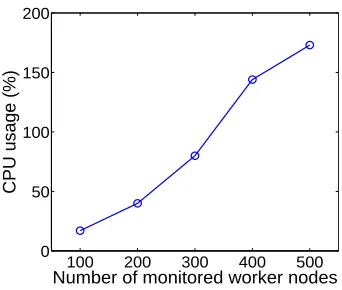
However, it is a challenging task to deploy fine-grained monitoring for large-scale hosting infrastructures due to the scalability concern. A production hosting infrastructure often com-prises thousands of physical hosts and many more virtual machines (VMs), each of which can be associated with hundreds of dynamic metrics [5, 10]. For example, the IBM Tivoli monitor-ing system [10] can collect over 600 metrics on a smonitor-ingle host. Hence, most production hostmonitor-ing infrastructures [5, 15] typically use a long update interval (e.g., every five minutes) to avoid ex-cessive monitoring overhead. Figure 2.4 shows the CPU usage of a dual-core 2.4GHz server that monitors different numbers of worker nodes. Here, we assume that each worker node reports 90 intra-node attributes and 10 inter-node attributes at one second sampling interval to the management server. The size of each attribute is 8 bytes. We use the web workload generator httperf [9] to emulate different monitoring workloads. Figure 2.4 shows that the management node is almost overloaded when the number of worker nodes becomes large (e.g., 500). Thus, without reducing the monitoring traffic to the management node, it is impractical to apply fine-grained monitoring to large-scale hosting infrastructures.

(25)

Furthermore, the monitoring system should be failure-resilient in order to handle node and network failures.

(26)

Chapter 3

Online Anomaly Prediction Models

and Case Studies

In this chapter, we present a set ofonline anomaly prediction models that aim at raising alerts in advance before anomalies actually happen. We first develop two Bayesian classifier based prediction models that combine the attribute value prediction (Markov chain model) and the statistical classification methods (naive Bayesian classifier or tree-augmented Bayesian network-s). We achieve anomaly prediction by performing classification over predicted attribute values. We also develop a decision tree based prediction model that introduces an additionalalert state other than normal and anomaly states. The prediction model raises advance alerts when the system is classified as the alert state that precedes the anomaly state. Moreover, we present comprehensive measurement studies to quantify the predictability of different real-world per-formance anomalies by using those anomaly prediction models.

In the following sections, we ﬁrst present the preliminary information about the system data collection and labeling, which serve as the training data for anomaly prediction model learning. We then discuss the system design of two types of online anomaly prediction models: Bayesian classiﬁer based prediction model and decision tree based prediction model. Next, we describe the implementation and discuss experimental evaluation results. Finally, we summarize the work.

3.1 Preliminary

(27)

Figure 3.1: Bayesian classiﬁer based anomaly prediction model.

under normal experiment runs, as well as under the injection of a variety of faults that lead to anomalies.

We employ an anomaly detection module to annotate all measurement samples with either “normal” or “anomaly” class labels. A simple anomaly detection module can use anomaly predicates [44] based on the user’s service level objective (SLO) requirements. For example, we can use an anomaly predicate “processing time>50 milliseconds” to check whether the system is in the anomaly state or not. Previous work also provided more advanced anomaly detection schemes that can accurately distinguish anomaly from application workload change [34] and infer the anomaly labels using similarity clustering [38].

Speciﬁcally, let x⃗t denote a measurement sample, which is a vector of k system attribute values [x0, . . . , xk] sampled at timet. Let Ct denote the class label at time t1, which can take one of the two states {abnormal(1), normal(0)}. Therefore, a time-series of recent collected measurement sample with appropriate class labels, denoted as ⟨x⃗t, Ct⟩, are used as the input training data for building the anomaly prediction models that will be discussed below.

3.2 Bayesian Classifier Based Anomaly Prediction Model

3.2.1 Approach Overview

We use Bayesian classifiers as the statistical anomaly classifiers to categorize the current system state into either normal or anomaly state based on the current measurement samples. To achieve advance prediction, we combine the statistical anomaly classifiers with the attribute value predictor. Thus, the models perform anomaly classification on future predicted attribute values with different probabilities to forecast the system anomaly state in the near future.

1

(28)

0.5

0.3

0.2 0.3

0.3

0.2

0.5 0.2

0.5

Bin 1 [0,5]

Bin 2 [6,20]

Bin 3 [21,30]

Figure 3.2: The state transition diagram of the Markov chain model for an attribute. This attribute ranges from 0 to 30. We discretize the attribute values into three states. Each directed arc is labeled with the corresponding state transition probability.

Figure 3.1 presents the system design of the proposed anomaly prediction model. We use discrete-time Markov chain to build future value prediction model for each attribute. We use two different types of Bayesian classifiers as the statistical anomaly classifier: the naive Bayesian classifier and the tree-augmented naive Bayesian network (TAN). We then combine the attribute value predictor and the statistical anomaly classifier to construct the integrated anomaly pre-diction model.

3.2.2 Design Details

Attribute Value Prediction Model

We use ﬁnite discrete-time Markov chain (DTMC) to build an attribute value prediction model for each collected resource attribute. The model makes future prediction by evaluating the probabilities of all possible values that the attribute can take at a future time unit. We use two diﬀerent types of DTMC: the basic Markov chain and the two-dependent Markov chain in this work.

(29)

We assume that the Markov chain in our work is homogeneous. Therefore, we can derive the probability distribution of attributex at a future time instance by applying the Chapman-Kolmogorov equation [80]. Speciﬁcally, let tdenote the number of steps away from the current time. The step interval is a ﬁxed value (e.g., 5 seconds). Aftertsteps, the probability distribution of attribute x is πt =πt₋1Px =πt₋2P_x2 =...= π0P_xt, where πt and π0 denote the probability distribution intsteps and the initial probability distribution of attributex, respectively. Given the current state i, if we want to predict the state at a future step t, we need to check the elements of matrix πt =π0P_xt at row i and decide the most likely future state (i.e., the state with the largest probability).

To use the discrete-time Markov chain, we need to perform data discretization that divide the range of a continuous attribute into a number of bins. Each bin represents a discrete state that can be used to replace actual attribute values. Traditional discretization techniques include equal width and equal depth binning. The equal width binning divides the attribute range into intervals of equal size. The equal-depth binning divides the attribute range into multiple intervals, each containing approximately same number of samples. However, in our experimental studies, we ﬁnd that both approaches will incur high prediction errors.

To reduce prediction errors of Markov chain model, we propose a hybrid discretization approach. We first use the equal-width binning approach to createMbins. We check the number of data samples that fall into each bin. If there is no bin containing too small number of data samples (e.g. less than 10% of the second smallest bin), the discretization is accepted. Otherwise, we apply the equal-width binning approach again but create more bins (e.g. 2M). Then we recursively merge some bins into their neighboring bins. In each iteration, we process the bin that currently contains the smallest number of data samples. We repeat such process until the total number of bins has been reduced to the target number M. This hybrid discretization approach has two benefits: First, it preserves the original continuous attribute distribution; Second, it mitigates the negative effect of some outliers by leverage the idea of equal depth binning to balance the number of data samples allocated to each bin.

(30)

11 13

31

12

23

33 32

22 21

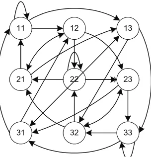
Figure 3.3: Two-dependent Markov model for attribute value prediction.

prior state that is one step earlier than the current state. Thus, it can resolve the ambiguity of making future predictions in the previous example. In general, two-dependent Markov model can improve prediction accuracy for those attributes that have large ﬂuctuations. Figure 3.3 shows the state transition diagram of a two-dependent Markov chain model for an attribute that is discretized into three single states. In this example, we construct nine combined states after merging every two single states to transform this non-Markovian attribute into the Markovian one.

We periodically update the Markov models with new measurement samples to adapt to dynamic systems. It is possible to use other prediction methods such as Kalman ﬁlter to predict attribute values at a future time. We choose the discrete-time Markov chain in this work because it can provide the probabilities of all possible values an attribute can take at a future time. Thus, we can easily integrate the probabilistic attribute value prediction results with the Bayesian series of classiﬁers to assess the probability of anomaly occurrence at a future time.

Statistical Anomaly Classiﬁcation

The goal of the anomaly classifier is to decide whether the system is currently in a normal or abnormal state. Ideally, the anomaly classifier should be able to produce posterior probabilities, i.e. P(C = 1|⃗x) and P(C = 0|⃗x) for a given measurement ⃗x. We then compare the posterior probabilities forabnormal andnormal classes to decide the classification result. The system is classified as abnormal if the following inequality holds:

(31)

C

1 2 3 4

X X X X

Figure 3.4: Naive Bayesian classiﬁer.

C

X1

2

3

4

X

Figure 3.5: TAN classiﬁer.

Otherwise, the system is classified to be in the normal state. Larger δ denotes stronger classi-fication confidence since the likeliness of one class is overwhelmingly greater than that of the other class. A typical value of δ is either zero or the prior difference of the likelihood derived from the training dataset.

However, computing the posterior probability is challenging: we need to evaluateP(C =c|⃗x) for every possible⃗xin the multidimensional attribute space. If the dimensionality is high, such computation will be very costly. To address this problem, we leverage the Bayesian theorem to convert the posterior probability P(C = c|⃗x) into the conditional probability P(⃗x|C = c). We use naive Bayesian classiﬁer [69] and tree-augmented naive Bayesian (TAN) network [47] in this work.

Naive Bayesian Classifier. For the naive Bayesian classiﬁer, each attribute is indepen-dent given the class label, which is illustrated by Figure 3.4. To computeP(C=c|⃗x), we apply the Bayesian theorem to transform the posterior probability into the conditional probability as follows:

P(C=c|⃗x) = P(⃗x|C =c)P(C=c)

P(⃗x) (3.2)

We can ignore the denominatorP(⃗x) that does not depend onC and only focus on the numer-ator. We then apply the naive independence assumption. Thus, we transform P(⃗x|C =c) into

∏n

i=1P(xi|C=c).

(32)

Bayesian classiﬁer, not all attributes are independent now. We applied an existing scheme [35] for the TAN model learning. For example, we can derive the following proportional relations for the TAN model shown in Figure 3.5: P(C=c|⃗x)∝P(x1|C =c)P(x2|C =c, x3)P(x3|C= c, x1)P(x4|C =c, x3).

The posterior probability P(C=c|⃗x) is proportional to the probability thatC is assigned with “abnormal” or “normal” label. We use the odds ratio [45], which is denoted by Ω(⃗x), to decide how to assign class labels to a sample vector⃗x. Speciﬁcally, the system is classiﬁed as abnormal if the following inequality holds:

Ω(⃗x) = P(C = 1|⃗x)(1−P(C= 0|⃗x))

P(C = 0|⃗x)(1−P(C= 1|⃗x)) > α (3.3) The thresholdαis a tunable parameter that can be used to control the classiﬁcation conﬁdence. A typical value ofα is one.

Integrated Anomaly Prediction

To achieve advance anomaly prediction, we integrate the attribute value prediction with the statistical anomaly classification. By using the attribute value prediction model, we can predict the values of each attribute at a future time. The anomaly classifier is then used to perform classification over future predicted attribute values. Specifically, during the computation of conditional probabilities in naive Bayesian or TAN classifier, we need to replace the attribute values in Equation 3.2 and Equation 3.3 with the predicted attribute values in the form of different probabilities that are obtained from the attribute value prediction model.

For the naive Bayesian classiﬁer, we need to replace the deterministic discrete value of xi with all possible discrete values thatxi can take. We denoteP(xi[s, t]) as the probability thatxi takes valuesat a future timet, given the current value of xi. Therefore, P(xi|C=c) becomes

∑

sP(xi[s, t])·P(xi[s, t]|C = c). Since we build Markov prediction model separately for each collected attribute, we aggregate all attributes in⃗xto get the predicted posterior probabilities

ˆ

P(C =c|⃗x) and use Equation 3.1 to get the anomaly prediction result.

(33)

Figure 3.6: Tunable anomaly predictor with diﬀerent alert intervals.

probability ˆP(C = c|⃗x) and use the odds ratio deﬁned in Equation 3.3 to get the anomaly prediction result.

3.3 Decision Tree Based Anomaly Prediction Model

3.3.1 Approach Overview

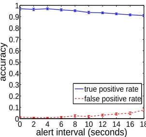
This anomaly prediction model uses a decision tree classifier that can continuously classify each measurement sample intonormal, alert, or anomaly state. Different from a traditional decision tree classifier that only generates binary classification results, we introduce a specialalertstate to capture system pre-anomaly symptoms. To achieve prediction, the model raises advance alerts when the system is classified as the alert state that precedes the anomaly state.

Figure 3.6 shows the decision tree classifiers with different configurations. We can see that the alert state corresponds to a region that precedes the data samples with “anomaly” labels in the multidimensional attribute space.

3.3.2 Design Details

Diﬀerent from the normal and abnormal measurement samples that are labeled by the anomaly detector, the labeling process for the alert state is controlled by a parameter calledalert interval

(34)

Figure 3.7: Anomaly prediction using a decision tree classiﬁer.

will classify more measurement samples as alert state than those in Figure 3.6(b). Intuitively, the larger the alert interval is, the more measurement points will be classiﬁed as “alert” and thus the more likely the predictor is to raise anomaly alerts. We can use the alert interval I as a tuning knob to control the predictor’s performance. At one extreme, if we set I = 0, ALERT becomes a conventional reactive approach where the alert state is always empty and no alert will be generated until the anomaly happens. At the other extreme, if we set I =∞, ALERT becomes a traditional proactive approach that performs preventive actions on all components unconditionally. The optimal solution often lies in-between the two extremes in practice, which motivates us to develop tunable prediction models. The alert interval can be used to tune the tradeoﬀ between true positive rate and false alarm rate.

(35)

Table 3.1: Subset of monitored attributes.

PlanetLab Attributes Description

Load1 load in last 1 minute

Load5 load in last 5 minutes

AvailCPU percentage of free CPU cycles

Myfreedisk free disk space of my slice

Disk usage percentage of utilized disk space

Freedisk free disk space

Freemem available memory

Numslice num. of registered slices on this host

SMART Attributes Description

Temp current internal temperature

Servo servo motor status

CSS total number of drive start/stop cycles

ReadError a rate at which read retries are requested

WriteError a rate at which write retries are requested

FlyHeight height of heads above the disk surface

System S Attributes Description

AvailCPU percentage of free CPU cycles

Freemem available memory

Page in/out virtual page in/out rate

Myfreedisk free disk space

Rxsdos num. of received data objects

Txsdos num. of transmitted data objects

Dpsdos num. of dropped data objects

Rxbytes num. of received bytes

Txbytes num. of transmitted bytes

Queuelen input queue length

Utime process time spent in user mode

Stime process time spent in kernel mode

Vmsize address space used by a component

Vmdata VM usage of the heap

Vmstk VM usage of the stack

3.4 Implementation and Evaluation

In this section, we evaluate the proposed online anomaly prediction models. We conduct com-prehensive measurement studies on three real-world systems. We ﬁrst describe the anomaly data collection. We then present the evaluation metrics for online anomaly prediction. Finally, we present and discuss the experimental results.

3.4.1 Anomaly Data Collection

(36)

several real-world computing infrastructures such as PlanetLab [82], NCSU virtual computing lab (VCL) [15], and IBM System S stream processing cluster [49]. One key challenge for this measurement study is to collect real system anomaly data from deployed production systems. Although previous research work have collected various failure data [6], most of them lack ﬁne-grained continuous measurement data that are required by the anomaly prediction model. One exception is the SMART disk failure data [76], which have been included in our measurement study. To collect more ﬁne-grained real-world system anomaly data, we developed a scalable monitoring system [114] and deployed it on the PlanetLab, VCL, and IBM System S. We col-lected a set of real system anomaly data by monitoring those systems for an extended period of time. We did not explicitly perform feature selection, which means that all the collected attributes are used for the training process of our anomaly prediction models. Table 3.1 lists a subset of monitored attributes collected on PlanetLab, SMART dataset, and System S. We describe the anomaly trace data collection in details as follows.

PlanetLab anomaly data.We collected measurement data on the widely used planetary-scale open computing platform PlanetLab. We monitored about 400 PlanetLab nodes distribut-ed all over the world. Our system collects 66 host attributes such as CPU load, virtual memory states, disk usage, and network traﬃc. The detailed description about those attributes can be found on either PlanetLab monitoring site [5] or our InfoScope monitoring site [11]. The at-tribute sampling interval is 10 seconds. We started the data collection since January 2009. The dataset used in our experiments was collected from Nov. 14th to Nov. 24th, 2009.

Our monitoring infrastructure can capture three types of node anomalies: 1) ping failure: a host is not responsive to consecutive five ping attempts initiated by the management node; 2) SSH failure: a node can not be accessed by the “ssh” command; and 3) monitoring sensor failure: the monitoring sensor program running on that node crashes and cannot be restarted. Each detected failure is recorded in a failure log with the node name and the timestamp of failure occurrence. The system stores monitored attribute data received from different nodes in separate log files. We then correlate the failure log with the monitored attribute logs for data labeling. We label 100 data samples before each failure occurrence as “abnormal” and other data samples as “normal”.

(37)

occurrences for those failed disks.

In the SMART dataset, one data sample originally consists of 59 attributes. We remove those attributes that are obviously not useful for prediction, such as serial number, frame number, and hours.

IBM System S anomaly data.We collected the third anomaly trace on the IBM System S [49], a large-scale data stream processing system running on a commercial cluster consist-ing of about 250 blade servers. We run a complicated multimodal stream analysis reference application [46]. We collected 21 system metrics with the sampling interval of two seconds. The system anomalies include bottleneck anomaly, throughput anomaly, and processing time anomaly. Those anomalies are caused by various reasons such as memory leak, CPU starvation, and buﬀer management error.

3.4.2 Evaluation Metrics

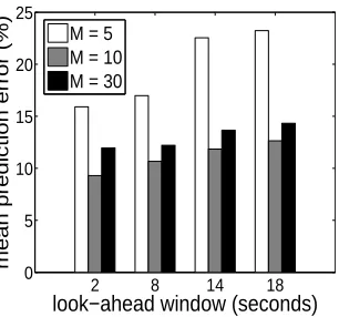
First, we evaluate attribute value prediction accuracy of the Markov chain model used in Bayesian classifier based anomaly prediction model. We use the prediction error to measure the difference between a predicted continuous attribute value and its corresponding true con-tinuous attribute value. Specifically, we assume thatx(t) is the sampled continuous value of an attribute x at the current time t. Its corresponding discrete state is denoted as s(t). On one hand, the attribute prediction model can predict the discrete state s′(t+T) with a look-ahead windowT (i.e., how far the model looks into the future). We then convert s′(t+T) to the pre-dicted continuous valuex′(t+T) by calculating the average value of all attribute measurement samples in the bin that corresponds to the discrete state s′(t+T). This means that x′(t+T) is the representative value of bin s′(t+T). On the other hand, we know the true continuous attribute value at timet+T, which is denoted asx(t+T). We then calculate themean predic-tion error (MPE) of the attribute x under the look-ahead windowT by traversing the testing datasetD as follows:

M P E(T) =AV GD

(

|x(t+T)−x′(t+T)| x(t+T)

)

(3.4)

(38)

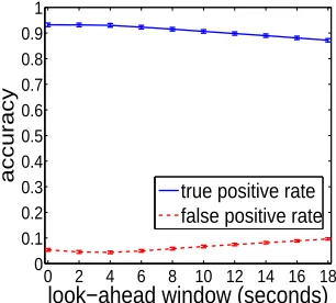
evaluate the performance of the decision tree classiﬁer using the ROC curve. The reason is that the decision tree classiﬁer is designed to produce only a binary class decision (i.e., “abnormal” or “normal”) on each data sample. Thus, it only produces a singe point in ROC space.

Third, and most importantly, we evaluate the overall prediction accuracy of the proposed online anomaly prediction models by using the standard true positive rateAtpand false positive rate Af p metrics. For the Bayesian classiﬁer based prediction model, let t denote the current time and T denote a speciﬁc look-ahead window. Based on the current measurement sample ⃗

xt, the prediction model will predict a class label ˆCt+T with look-ahead window T. Note that we also know the true label Ct+T that has been annotated for the measurement sample⃗xt+T. We then compare this true label with the predicted label for veriﬁcation.

For the decision tree based prediction model, we have an additional “alert” class label that is conﬁgured by the alert intervalI during the model training phase. During the testing phase, we compare the predicted label ˆCt with the true label Ct for each measurement sample ⃗xt at timet. Note that we treat the “alert” class label as the same as the “anomaly” label.

Therefore, by comparing the predicted label with the true label, we have four possible cases: 1) If the predicted label is ”anomaly” and the true label is also “anomaly”, the prediction is a true positive (TP); 2) If the predicted label is “anomaly” but the true label is “normal”, the prediction is a false positive (FP); 3) If the predicted label is “normal” but the true label is “anomaly”, it is a false negative (FN) and 4) If the predicted label is “normal” and the true label is also “normal”, the prediction is a true negative (TN). We denote Ntp, Nf p, Nf n, and Ntn as the number of TP, FP, FN, and TN respectively. We then calculate the true positive rate Atp and false positive rateAf p in a standard way as follows.

Atp =

Ntp Ntp+Nf n

, Af p=

Nf p Nf p+Ntn

(3.5)

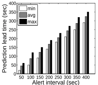
Finally, we measure the prediction lead time achieved by our online anomaly prediction models, which means how early the model can raise advance alerts before anomaly occurrences. The lead time is calculated as the difference between the time when the first alert was raised and confirmed before an anomaly occurrence and the time when this anomaly occurred.

3.4.3 Results and Analysis

(39)

10 40 70 90 0

5 10 15 20 25

look−ahead window (seconds)

mean prediction error (%)

equal−depth hybrid equal−width

Figure 3.8: Markov prediction error for PlanetLab data: quantization scheme.

10 40 70 90 0

5 10 15 20 25

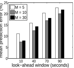
M = 5 M = 10 M = 30

Figure 3.9: Markov prediction error for PlanetLab data: quantization granularity.

under diﬀerent look-ahead windows. After that, we compare the prediction accuracy of the basic Markov chain model and the two-dependent Markov chain model. In the end, we report the overhead of those anomaly prediction models.

PlanetLab Anomaly Prediction

We first examine the failure data collected on the PlanetLab. We focus on the host ping failures since we find that SSH failures and sensor program startup failures are rare. Host ping failures occur frequently on the PlanetLab but with various frequencies and durations on different PlanetLab hosts. We detected ping failures on around 400 PlanetLab nodes. The average number of ping failure occurrences for each node during the monitoring period is 15. The average duration of ping failures is 6 hours. For each host, we use the first half of the data as the training dataset and the second half as the testing dataset.

(40)

0 0.2 0.4 0.6 0.8 1 0

0.1 0.2 0.3 0.4 0.5 0.6 0.7 0.8 0.9 1

false positive rate true positive rate _{node1: ece.uprm.edu}

node2: scsr.nevada.edu

Figure 3.10: Classiﬁcation ROC curves for PlanetLab data: naive Bayesian.

0 0.2 0.4 0.6 0.8 1

0 0.1 0.2 0.3 0.4 0.5 0.6 0.7 0.8 0.9 1

false positive rate true positive rate _{node1: ece.uprm.edu}

node2: scsr.nevada.edu

Figure 3.11: Classiﬁcation ROC curves for PlanetLab data: TAN.

large. On the other hand, with a large number of bins (e.g.,M = 30), each bin will be assigned with less number of training data. If the training dataset is not large enough, the Markov chain model will be get insuﬃciently trained. Thus, the predictor will make mistakes when predicting the bin number that an attribute should belong to, which will also incur large attribute value prediction errors.

We then evaluate the performance of the naive Bayesian classifier and the TAN classifier. Note that when we use the anomaly classifier without combining the attribute value predictor, we do not predict into the future. We only determine whether the system at the current time exhibits abnormal behaviors. Figure 3.10 and Figure 3.11 show the ROC curves of classifying ping failures on two specific PlanetLab hosts. For an ROC curve, the optimal performance should be at the top left where the classifier achieves the highest true positive rate and the lowest false positive rate. We observe that both classifiers have good performances. Furthermore, the TAN classifier performs slightly better than the naive Bayesian classifier.

We evaluate the performance of two Bayesian classifier based anomaly prediction model un-der different look-ahead windows in Figure 3.12 and Figure 3.13. We average the results among five PlanetLab hosts and include the standard error bars for both true and false positive rates. We have several observations: 1) The models can still achieve reasonably good prediction accura-cy for future system state; 2) Prediction accuraaccura-cy gradually decreases as the look-ahead window becomes larger, which implies that predicting anomalies in more distant future is challenging; 3) TAN classifier can achieve higher prediction accuracy than the naive Bayesian classifier. The performance degradation is also less when the length of the look-ahead window increases; and 4) Both models are stable with small standard errors, which implies the anomaly prediction algorithms are robust for node failures occurred on different hosts.

(41)

0 10 20 30 40 50 60 70 80 90 0

0.1 0.2 0.3 0.4 0.5 0.6 0.7 0.8 0.9 1

look−ahead window (seconds) accuracy true positive rate

false positive rate

Figure 3.12: Advance anomaly predic-tion accuracy for PlanetLab data: naive Bayesian + Markov.

0 10 20 30 40 50 60 70 80 90 0

0.1 0.2 0.3 0.4 0.5 0.6 0.7 0.8 0.9 1

accuracy

true positive rate false positive rate

Figure 3.13: Advance anomaly predic-tion accuracy for PlanetLab data: TAN + Markov.

0 10 20 30 40 50 60 70 80 90 0

0.1 0.2 0.3 0.4 0.5 0.6 0.7 0.8 0.9 1

alert interval (seconds) accuracy true positive rate

false positive rate

Figure 3.14: Advance anomaly prediction accuracy for PlanetLab data: decision tree classiﬁer.

(42)

2 8 14 18 0

5 10 15 20

look−ahead window (hours)

Figure 3.15: Markov prediction error for SMART data: quantization scheme.

2 8 14 18

0 10 20 30 40

look−ahead window (hours)

M = 5 M = 10 M = 30

Figure 3.16: Markov prediction error for SMART data: quantization granularity.

SMART Anomaly Prediction

We now present the anomaly prediction results for the SMART dataset. We split the original SMART dataset into six subsets, each of which contains different failed and normal disks. We conduct six-fold cross-validation for all the experiments. First, we show the impact of different configuration parameters on the accuracy of the basic Markov predictor in Figure 3.15 and Figure 3.16. Again, we observe that our hybrid discretization approach consistently performs better than the other two approaches. Particularly, the equal-width discretization incurs much higher prediction error than the other two approaches. The reason is that the range of some SMART attributes is very large. The equal-width discretization tends to make the range of each bin very big. Therefore, one specific data sample might be numerically far away from the representative value of the bin that it belongs to, especially when the bin only contains a small number of data samples. Similarly, we achieve the lowest prediction error when M is neither too small nor too large. For the same reason we have discussed above, the prediction accuracy when the number of the bin is equal to 5 is much worse than the other two cases.

(43)

0 0.2 0.4 0.6 0.8 1 0 0.1 0.2 0.3 0.4 0.5 0.6 0.7 0.8 0.9 1

false positive rate true positive rate worst subset_average

best subset

Figure 3.17: Classiﬁcation ROC curves for SMART data: naive Bayesian.

0 0.2 0.4 0.6 0.8 1

0 0.1 0.2 0.3 0.4 0.5 0.6 0.7 0.8 0.9 1

false positive rate true positive rate worst subset_average

best subset

Figure 3.18: Classiﬁcation ROC curves for SMART data: TAN.

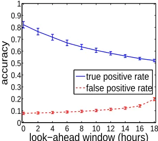
0 2 4 6 8 10 12 14 16 18 0 0.1 0.2 0.3 0.4 0.5 0.6 0.7 0.8 0.9 1

look−ahead window (hours) accuracy _{true positive rate} false positive rate

Figure 3.19: Advance anomaly prediction accuracy for SMART data: naive Bayesian + Markov.

0 2 4 6 8 10 12 14 16 18 0 0.1 0.2 0.3 0.4 0.5 0.6 0.7 0.8 0.9 1

look−ahead window (hours) accuracy true positive rate false positive rate

Figure 3.20: Advance anomaly predic-tion accuracy for SMART data: TAN + Markov.

other attributes. In the SMART dataset, some attributes have a large value range and the number of data samples inside diﬀerent bins can be very imbalanced. Thus, the estimation of some conditional probabilities become inaccurate when some of the bins contain very few training samples. However, this problem is not so acute in the case of the naive Bayesian classiﬁer since it assesses the conditional probability only based on the class variable, and the values of the class variables are adequately represented in the SMART dataset.

(44)

2 8 14 18 0

5 10 15 20

Figure 3.21: Markov prediction error for System S data: quantization scheme.

2 8 14 18

0 5 10 15 20 25

M = 5 M = 10 M = 30

Figure 3.22: Markov prediction error for System S data: quantization granularity.

hours.

We do not report the prediction accuracy results of the decision tree based prediction model for the SMART dataset. The reason is brieﬂy explained as follows. In the SMART dataset, each good disk only has the time series samples labeled as “normal”. Similarly, each failed disk only has the time series samples labeled as “abnormal”. There is no disk that contains a segment of “normal” samples followed by a segment of “abnormal” samples. Therefore, we cannot apply an alert interval to label some data samples before disk failures as “alert”.

System S Anomaly Prediction

We now present the anomaly prediction results for the System S dataset. Diﬀerent from the previous two systems, this set of experiments focus on performance anomalies (e.g., prolonged processing time, low system throughput) caused by various faults such as insuﬃcient resources and program bugs. We collected data from six densely-coupled hosts. These six hosts have very similar application behavior in the experiments so that we can use six-fold cross-validation to improve the prediction model accuracy.

Figure 3.21 and 3.22 show the attribute value prediction accuracy of the basic Markov chain model under diﬀerent discretization schemes and quantization granularity, respectively. Again, we observe that the hybrid discretization scheme using 10 discrete bins achieves the lowest prediction error.