©
DOI: 10.1534/genetics.104.032276
The Structured Ancestral Selection Graph and the Many-Demes Limit
Paul F. Slade*
,1and John Wakeley
†*School of Mathematics and Statistics, School of Biological Sciences, SUBIT, University of Sydney, New South Wales 2006, Australia and †Department of Organismic and Evolutionary Biology, Harvard University, Cambridge, Massachusetts 02138
Manuscript received June 21, 2004 Accepted for publication October 28, 2004
ABSTRACT
We show that the unstructured ancestral selection graph applies to part of the history of a sample from a population structured by restricted migration among subpopulations, or demes. The result holds in the limit as the number of demes tends to infinity with proportionately weak selection, and we have also made the assumptions of island-type migration and that demes are equivalent in size. After an instantaneous sample-size adjustment, this structured ancestral selection graph converges to an unstructured ancestral selection graph with a mutation parameter that depends inversely on the migration rate. In contrast, the selection parameter for the population is independent of the migration rate and is identical to the selection parameter in an unstructured population. We show analytically that estimators of the migration rate, based on pairwise sequence differences, derived under the assumption of neutrality should perform equally well in the presence of weak selection. We also modify an algorithm for simulating genealogies conditional on the frequencies of two selected alleles in a sample. This permits efficient simulation of stronger selection than was previously possible. Using this new algorithm, we simulate gene genealogies under the many-demes ancestral selection graph and identify some situations in which migration has a strong effect on the time to the most recent common ancestor of the sample. We find that a similar effect also increases the sensitivity of the genealogy to selection.
K
IMURA (1983) strongly promoted the idea that the Hudson (1983), and Tajima (1983). The reason forabundant genetic variation seen in nearly every spe- this is clear: it is much simpler to predict the frequencies
cies studied must be neutral.OhtaandKimura(1971) of selected alleles using diffusion theory than using the
suggested a less strict version of this in which polymor- backward-time approach of the coalescent. For neutral
phisms are explained by the constant input of nearly loci, the coalescent provides a simple and useful
descrip-neutral mutations,i.e., variants with selective advantages tion of the genetic ancestry of a sample of genetic data— or disadvantages smaller than the reciprocal of the pop- the genealogy for short—from a large well-mixed, or pan-ulation size. After a great deal of debate and many analy- mictic, population of constant size through time. Due to
ses, summarized inGolding(1994), there are now few the close connection between genealogies and genetic
adherents to the strict neutral mutation hypothesis. Mo- data, and to the ease with which genealogies can be
sim-lecular techniques currently allow huge numbers of ulated, a growing set of computational tools use the
coales-polymorphisms to be assayed with relative ease, and the cent to make inferences about population history from
resulting genomic data can be used to estimate the DNA sequences; seeStephens(2001) andTavare´(2004)
strength of selection associated with genetic differences for reviews.
(Sawyer and Hartl 1992; Bustamante et al. 2002). The coalescent is robust to many kinds of deviations
Recent statistical inferences made from such data em- from its underlying assumptions (Kingman1982b;Mo¨ hle
phasize the importance of selection and show that selec- 1998c), but it does not hold when members of the
sam-tive advantages or disadvantages on the order of the ple, or the ancestral lineages of the sample, are not
reciprocal of the population size may be fairly common
exchangeable. In fact, the relative simplicity of the neu-(Sawyeret al.2003).
tral coalescent process flows directly from the exchange-The methods used in these works to estimate selection
ability of the lineages. Exchangeability, which results parameters from intraspecific genomic data rely on
pre-in the model from the assumptions of neutrality and dictions of sample allele frequencies derived from
for-panmixia, means that the statistical properties of a sam-ward-time diffusion theory. They do not use the
ances-ple do not depend on how the samances-pled items are labeled tral genetic process known as the coalescent, which was
(Kingman 1982b; Aldous 1985). Possible “labels”
in-introduced in the early 1980s byKingman (1982a,b),
clude the geographic locations where the samples were collected or the allelic states of the samples if these are known. When samples are not exchangeable, a related
1Corresponding author:School of Mathematical Sciences, University
of Adelaide, SA 5005, Australia. E-mail: [email protected] but more complicated model called the stuctured
lescent exists (Slatkin 1987; Strobeck 1987; Noto- able to identify cases in which simple models may be applied even though the underlying dynamics appear
hara1990;Wilkinson-Herbots1998), and
computa-tional methods of inference are being developed for complicated. We present a rigorous derivation of the
ASG with very many demes (subpopulations) in an
is-this model as well (NathandGriffiths1996;Beerli
and Felsenstein 1999, 2001; Bahlo and Griffiths land model of migration (Wright1931) and show that it possesses a simple structure akin to that under
neutral-2000;De IorioandGriffiths2004).
Genealogies in the presence of strong selection,i.e., ity (Wakeley1998). Five parameters collapse into just
three (one each for migration, selection, and mutation) with selective advantages or disadvantages much greater
than the reciprocal of the population size, can be mod- in the limit as the number of demes tends to infinity.
Interestingly, the population rates of selection and mu-eled using the structured coalescent with the
subdivi-sions being the alternative alleles (Kaplan et al. 1988, tation scale differently (see below) in the presence of population subdivision. This was found previously in
1989). For weak selection, Krone and Neuhauser
(1997) andNeuhauserandKrone(1997) showed that forward-time analyses (Wakeley 2003; Wakeley and
Takahashi2004), but the result is more intuitive in the the genealogy of a sample taken at random with respect
to allelic variation is described by an exchangeable an- present case. We also describe a newly enhanced process
for the simulation of genealogies conditional on the cestral process. The ancestral selection graph (ASG) is
a branching-coalescing random graph within which the frequencies of alleles in the sample. We show using
con-ditional simulations that population subdivision and mi-simple, bifurcating genealogy of a sample is embedded.
The elegant exchangeability of the ASG comes with a cost: gration among very many demes accentuate the action
of selection on the genealogy. it lends itself only to very computationally intensive
tech-niques. In addition, there appears to be very little about genealogies in the ASG that differs greatly from
genealo-THEORY
gies under neutrality (KroneandNeuhauser1997).
For these reasons, and also to be able to control for The structured ancestral selection graph is the
ances-tral process for a class of forward-time models. Following sampling, recent extensions to the ASG have modeled
genetic ancestry conditional on the frequencies of se- KroneandNeuhauser(1997) we begin by describing
a continuous-time model in which reproduction occurs lected alleles in the sample (Slade2000a,b;Stephens
and Donnelly 2003; Bartonet al. 2004). This leads according to theMoran(1958, 1962) model, but where the population is subdivided into demes (subpopulations) to dramatic improvements in computation time while
preserving some degree of exchangeability among the connected by migration. There are D demes, and in a
general model these might have sizesNi,i⫽ 1, . . . ,D. sampled lineages (Slade2000a). The conditional
simu-lation of selected genealogies by Slade (2000a,b) en- We assume that each of the兺D
i⫽1Nilineages in the popu-lation can be in one of two possible allelic states, A1
ables the timing structure of common ancestry to be
quantified. In contrast to the unconditional ASG, gene- and A2, with relative rates of reproduction 1 and 2,
respectively. However, as in Krone and Neuhauser
alogies conditional upon allele frequencies in the
sam-ple may be either larger or smaller on average than gene- (1997), we begin with a description in which the states of lineages are not specified and so each lineage undergoes alogies under neutrality (Slade2000a); see also the review
ofSladeandNeuhauser(2003). The extent of these two kinds of reproduction (birth/death) events. Type 2 birth/death events occur with rate2⫺ 1per lineage.
differences depends strongly on the initial sample
con-figuration of alleles, particularly for small mutation These represent the action of selection since they are
realized only if the lineage that reproduces is of the rates. Under neutrality, samples in which there are
ap-proximately equal numbers of each allele have longer favored allelic type at the time of the event. Type ␦
birth/death events occur with rate1per lineage. The
times to common ancestry than more unbalanced
sam-ples. However, the selective effect on genealogies for sam- majority of birth/death events will be of this type, and they can be thought of as neutral in the sense that they ples in which there are approximately equal numbers of
each allele is greater than that of more unbalanced are realized regardless of the allelic type of the parental
lineage. Note that at this point, without specifiying the samples. We show that restricted migration can cause
unbalanced samples to be converted to balanced sam- allelic types, lineages are exchangeable within demes
but are not exchangeable between demes. Note also ples, via the instantaneous sample-size adjustment
men-tioned above, and thus the time to common ancestry that, while this is a model of directional selection, it is
possible to include frequency dependence (Neuhauser
under selection is reduced.
Our purpose is to consider the ASG in the presence 1999) or general diploid selection (Slade2000a).
Subdivision is mediated by a collection of D ⫻ D
of population subdivision and migration. Population
structure is evident in many genetic data sets but model- migration probabilities,mij, fori,j⫽ 1, . . . ,D. When
a lineage in deme j reproduces, either by a type ␦ or
ing it presents difficulties (Slatkin1985; Avise2000;
valu-formly at random from among theNilineages in deme Neuhauser(1997) refer to as the percolation diagram. This is shown in Figure 1 and is the structured analog i with probability mij. With probability 1 ⫺ m, where
m⫽ 兺D
i⫽1mij, the individual to die is chosen uniformly of Figure 1 inKroneandNeuhauser(1997). Following a single lineage, either forward or backward in time, at random from within the same deme as the
reproduc-ing individual. As usual in Moran-type models, the indi- 2-arrows are encountered at rate1sDand␦-arrows are encountered at rate1. Each arrow has a probabilitym
vidual chosen to reproduce might also be the one
cho-sen to die. Although the model does allow “migration” of connecting to a lineage sampled uniformly at random
from the entire population and probability 1⫺ m of
back to the same deme (with probabilitymii) the effect of
this becomes negligible in the large-Dlimit we consider connecting to a lineage sampled uniformly at random
from the same deme. Thus, there are four kinds of below.
The general model described above forms the basis branches and these appear repeatedly in the history of
every lineage with rates1(1 ⫺ m), 1m, 1sD(1 ⫺ m), for a structured ancestral selection graph. This would be
obtained via the usual large-Nlimit, withDfinite, in the and1sDm. Note that 1 is simply a scaling factor that
specifies the units in which time will be measured;1⫽
same way that the structured coalescent is obtained in
the neutral case (Notohara1990;Wilkinson-Herbots 1 corresponds to the usual notion of measuring time
in generations. 1998). That is, we would letN ⫽兺D
i⫽1Niand assume that
ci⫽Ni/N,Mij⫽Nimij, ⫽ 2⫺ 1, and ⫽Nu, where Thedualor ancestral process is obtained by following
lineages back in time, i.e., up the graph in Figure 1. uis the neutral mutation rate, are all finite asN →∞,
and time is measured in units ofNgenerations, where Because 2-arrows are realized only if the parental allele
is of the favored type, both lineages must be followed a generation is defined to be1⫺1time units. Note that
a crucial assumption of the structured coalescent is that in the ancestral process. A single genealogy is obtained, in the unconditional ancestral process, by tracing
lin-migration occurs only between theDdemes enumerated
in the initial sample, and the ancestry is therefore always eages back to the ultimate ancestor, assigning its type from the equilibrium distribution of allele frequencies restricted to those particular demes.
We do not pursue this large-Nlimit here, but instead (see below), and then following lineages forward in
time, with mutation, and trimming off branches appro-consider a limiting ancestral process that approximates
the behavior of a population divided into very many priately (KroneandNeuhauser1997;Neuhauserand
Krone1997). Rather than this unconditional ancestral demes and in which selective differences are small.
Thus, we assume that the sample size is small relative to process, we consider the genealogy of a sample contain-ing known numbers of different alleles. This leads to the number of demes in the population, rather than to
the deme size. Historically, migration can take ancestors more efficient simulation of selected genealogies. Using the conditional approach, it is possible to label ancestral to any deme within the population. This follows recent
coalescent work under the assumption of neutrality lineages as either virtualor real, and it is necessary to
trace lineages back only to the most recent common an-(Wakeley 1998) and work on the forward-time
diffu-sion approximation for allele frequencies in the pres- cestor of the sample,i.e., among thereallineages, rather than all the way back to the ultimate ancestor (Slade
ence of selection (Wakeley2003;Wakeleyand
Taka-hashi2004). We set 2 ⫽ (1 ⫹ sD)1, and we use 1sD 2000a). There is also a minimal representation of the ancestral process that reduces the number of possible in place of2 ⫺ 1 for the rate of type 2 birth/death
events below. This corresponds to a model in which events required at each ancestral transition (Sladeand
Neuhauser2003). We describe how this is done in the there are two alleles,A1andA2, and alleleA2has fitness
equal to 1⫹sDwhile A1has fitness equal to 1. We put present, structured model inmethodology.
The essence of the large-Dresult here, as in the neu-a subscript on the selection coefficient in recognition
of the fact that the limit we seek hasDs(andDu) finite tral case, is that the rates at which events occur that affect the history of a sample from the population are
asD→∞. FollowingLessardandWakeley(2004), the
large-N, large-Dlimit can also be studied. Similar limit very different when every lineage is in a separate deme than when at least one deme contains more than one results here require more stringent conditions: roughly,
thatDgoes to infinity faster thanN (seeappendix a). lineage. The dependence onDis such that a
separation-of-timescales result applies, as, for example, in Mo¨ hle
For simplicity, we assume that migration occurs
ac-cording toWright’s (1931) island model, but adapted (1998a,b). Because of this, the history of a sample can
be divided into two phases (Wakeley1999). The first
for Moran-type reproduction as inWakeleyand
Taka-hashi(2004). That is, we assume thatmij⫽m/Dfor all is a short scattering phase in which coalescent events occur between samples from the same deme and
migra-iandj, and thatNi⫽Nfor alli. Thus, we have a model
in which there areDdemes, each of size N, and each tion events in which lineages move to unoccupied demes
(i.e., demes that do not contain any ancestral lineages). of which receives a migrant from the total population
with probabilitymat each birth/death event. As in the The scattering phase occurs on a fast timescale and
be-comes an instantaneous sample size adjustment in the unstructured ancestral selection graph, it is helpful to
Figure1.—Graphical depiction of the struc-tured selection process for the case ofD⫽3 demes.
when all remaining lineages are in different demes. At used to show that the collection of demes is always
suf-ficiently close to that changes inX depend only on
this point, the collectingphase begins in which pairs of
lineages come together into a single deme and coalesce, the ensemble properties E[K]⫽ 兺Nk⫽0kk⫽Nx and
Var[K]⫽x(1⫺x)N2/(Nm ⫹1⫺m) and that the
dif-eventually finding a common ancestor of the entire
sam-ple. The migration events that could be ignored in the fusion ofXis identical to the usual unstructured
diffu-sion except that the timescale is increased by the factor scattering phase,i.e., those in which lineages move to
oc-cupied demes, are now essential since a coalescent event 1⫹(1⫺ m)/(Nm) (WakeleyandTakahashi2004).
By considering overall limiting rates of type ␦ and
can occur only between a pair of lineages if they are in
the same deme. We use the scattering/collecting termi- type 2 birth/death events—which are1NDand1sDND
(1⫺x), respectively—and conditioning on the number
nology even though we have incorporated selection.
Forward-time analysis:To simulate genealogies in both of copies of alleleA1in the deme where the
reproduc-tion event occurs, it can be shown that the conditional and the unconditional ASG, it is
neces-sary to know the equilibrium distribution of the frequen-cies ofA1andA2in the population. In fact, the ASG is
a model specifically for a sample from such an equilib-rium population. There will be no equilibequilib-rium without
mutation, and here we followKroneand Neuhauser
(1997) in assuming that there is a probability of muta- X→
⎧ ⎪ ⎪ ⎪ ⎪ ⎪ ⎨ ⎪ ⎪ ⎪ ⎪ ⎪ ⎩
X⫹ 1
ND with rate1NDx(1⫺x) Nm Nm⫹1⫺m
⫹ 1ND(1⫺x)uD
冤
1⫹2xNm Nm⫹1⫺m
冥
⫹O(sDuD)
X⫺ 1
ND with rate1NDx(1⫺x)(1⫹sD) Nm Nm⫹1⫺m
⫹ 1NDxuD
冤
1⫹2(1⫺x)Nm Nm⫹1⫺m
冥
⫹O(sDuD).
tionuDper birth/death event. We note that asymmetric
mutation can also be accommodated (Slade 2000a).
The forward-time dynamics of allele frequencies in a
(2) subdivided population may be complicated, but in the
case of a large number of demes they are nearly as simple
We let
as in an unstructured population (Wakeley2003). In
a model very similar to the one we consider here,
Wake-1⫽
ND 2
冢
1⫹1⫺m
Nm
冣
(3)leyandTakahashi(2004) showed that the frequencies of alleles in the total population change according to
and we further assume that a diffusion process that is identical to the diffusion
pro-cess in an unstructured population, only with a different NDs
D→ and NDuD[1⫹(1⫺ m)/(Nm)]→
timescale. Further, as these frequencies change (slowly)
asD→∞. (4)
the collection of demes closely tracks an equilibrium distribution of allele frequencies.
Then, the diffusion process for the frequency of allele
Let the random variable X(t) be the frequency of
A1 has drift parameter a(x) ⫽ ⫺(/2)x(1 ⫺ x) ⫹
alleleA1at timet, and letxrepresent a particular value (/2)(1⫺ 2x) and diffusion parameter b(x)⫽ x(1 ⫺
ofX(t). Because we consider the limitD→∞whileDsD
x). This process has a unique stationary distribution
andDuDremain finite, mutation and selection do not
appear in the equilibrium h(x)⫽ Bx⫺1(1⫺ x)⫺1e⫺x, (5)
whereBis a normalizing constant; that is,h(x) satisfies
k⫽
冢
N k冣冢
Nmx 1⫺m
冣
(k )冢
Nm(1⫺ x)
1⫺m
冣
(N⫺k)冒
冢
Nm 1⫺m
冣
(N)(1)
0⫽ 1
2 d2
dx2[b(x)h(x)]⫺
d
dx[a(x)h(x)] (6)
(Wakeley and Takahashi 2004), which here is the
fraction of demes in the population that containkcopies (Wright1949; Kimura 1955). With reference to
Fig-of alleleA1and in whicha(k)⫽a(a⫹1) · · · (a⫹k⫺1) ure 1, the two-part equilibrium (1) and (5), which
pre-is an ascending factorial. Clearly, the equilibrium vector dicts the distribution of A1 among demes and across
does depend on the frequency of alleleA1in the total the total population, is what would be observed by
as-population, and this will change over time. However, signingA1’s andA2’s to the lineages and then running
the process forward a very long time.
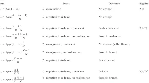
TABLE 1
The nine possible results of type␦and type 2 birth/death events in the history ofnlineages currently inndifferent demes
Rate Event Outcome Magnitude
U1⫽ 1n(1⫺m) ␦, no migration No change O(1)
U2⫽ 1nm
D⫺(n⫺1)
D ␦, migration to u-deme No change
U3⫽ 1nm n⫺1
D 1
N ␦, migration to o-deme, coalescent Coalescent event O(1/D)
U4⫽ 1nm n⫺1
D
N⫺1
N ␦, migration to o-deme, no coalescence Possible coalescent
U5⫽ 1sDn(1⫺m)
1
N 2, no migration, coalescent No change (self-collision)
U6⫽ 1sDn(1⫺m)
N⫺1
N 2, no migration, no coalescence Possible branch
U7⫽ 1sDnm
D⫺n
D 2, migration to u-deme Branch event
U8⫽ 1sDnm
n D 1
N 2, migration to o-deme, coalescent Collision O(1/D 2)
2, migration to o-deme, no coalescence Possible branch U9⫽ 1sDnm
n D
N⫺1 N
U-deme and o-deme mean unoccuppied deme and occupied deme, respectively.
The collecting phase: Consider the case in whichn coalescence as we follow the history of the sample back in time.
lineages are in, or are sampled from,ndifferent demes.
By tracing the lineages back in time without knowing It is appropriate that we have ignored mutations
above and in Table 1 because here we are dealing with their allelic types, we find a simple ancestral process in
the limitD→∞and generate an intuitive understanding the unconditional ancestral process. Mutations will
oc-cur with probability uD, 0 ⱕ uD ⱕ 1, at both types of for the different scaling of mutationvs.selection in (4)
and inWakeley(2003) andWakeleyandTakahashi arrows or reproduction events. Along a single lineage,
they occur with rate2uD⫽ND(1⫹sD)uD[1⫹(1⫺m)/ (2004). The four kinds of arrows, or reproduction events,
discussed above will be encountered by thesenlineages (Nm)]/2, which becomes/2 in the limitD→∞. As in
Krone and Neuhauser (1997) and Neuhauser and and will sometimes move them to occupied demes so
that they might coalesce. We can recognize nine possible Krone(1997), we superimpose this mutation process
on the unconditional ancestral process. In the conditional events for such a sample, and these are listed in Table 1.
For example, the fourth kind of event is that a␦-arrow ancestral process we consider below, it is necessary to treat mutation, coalescence, and branching simultaneously.
takes one of thenlineages to one of the othern ⫺ 1
occupied demes but does not connect to the resident When Dis large, the first two events in Table 1 will
account for the vast majority of events. These events ancestral lineage. The result is that now thenlineages,
while still distinct, reside inn⫺1 demes. Thus, at the have rates ofO(1), which here means that they have a
finite and nonzero limit asD→ ∞for a given1. It is
next event the two lineages that reside together in one
deme can coalesce. The interpretations of the other easy to see that this is true because the rates of these
events depend onDonly through1. These events are
events in Table 1 are equally straightforward. Note that
the events are categorized according to their effect on lineage switches within and between demes, but ones
that preserve the basic sample structure ofn lineages the ancestral lineages and also by their probabilities of
occurring with reference to the limit D → ∞ (while inndifferent demes. They do not change the rates at
which events occur and Table 1 continues to apply. DsD remains finite). As in the unstructured ancestral
selection graph, when a 2-arrow is encountered, both Note that with other kinds of (non-island) population
structure, these events would change the state of the paths are followed and the lineage splits into two
demes (Wakeley andAliacar 2001). Here, they can where
冢
n2
冣
⫽n(n⫺ 1)/2 and ⫽NDsD. Again, the firstbe ignored due to the symmetry of the island model. two types of events do not change the state of the sample,
The next most numerous events will be events 3–7, and so it is not problematic that their rates become infinite.
these have rates of O(1/D), which means that these It simply means that the ancestral lineages will
encoun-rates will approach zero as D → ∞for a given 1, but ter many birth/death events before anything of
rele-that their rate of approach to zero will be inversely vance happens to the sample. Event 3 is a coalescent
proportional toD. Again, the limiting process we seek event in which the number of lineages decreases from
is forDsDfinite asD→∞, so thatsDis ofO(1/D). Four nton⫺1 and thesen⫺1 lineages are all in different
of these events—3, 4, 6, and 7—do fundamentally alter demes. Event 7 is a branching event, in which case the
the state of the sample. These are migration events to sample goes fromnton⫹1 lineages, and a migration
occupied demes, both with and without coalescence, event leaves all n ⫹ 1 lineages in different demes. In
and branching events, both with and without a migra- event 4 the number of lineages remainsn, but now two
tion event to an unoccupied deme. of them are in the same deme, while in event 6 the
KroneandNeuhauser(1997) andNeuhauserand number of lineages increases to n⫹ 1, and again two
Krone(1997) use the termcollisionto denote the event are in the same deme. To summarize, the first step that
that an ancestral lineage splits and immediately co- matters in the limiting (D→∞) process forn lineages
alesces with another ancestral lineage. In the unstruc- in n different demes can be a coalescent event or a
tured ancestral selection graph, all collisions become branching event, but in either case the remaining
lin-negligible in the limit (N → ∞and D ⫽ 1), and it is eages are all in different demes; alternatively it can be
not necessary to distinguish between different kinds of a migration event or a branching event that results in
collisions. Here, becauseNis finite, some collisions will two lineages residing together in the same deme while
occur with rates comparable to regular coalescent events. the rest are in separate demes.
Event 5 in Table 1 is of this sort and has a rate ofO(1/ We note that Equations 13 and 14, correspond to
D). However, event 5 is a collision in which the lineage events that would disrupt the dual process or greatly
splits and then immediately coalesces with itself. Both complicate the branching structure, respectively. The
forward and backward in time, this has no effect. The zero rates with which we have described them above
descendant lineage has the same parent regardless of refer to their instantaneous rates in the limiting process,
whether the parental allele isA1and the 2-arrow is not but do not fully reveal that even over the entire graph,
followed or the parental allele isA2 and the 2-arrow is until the ultimate ancestor is reached, these events will
followed. We refer to this event as a self-collision. Only occur with probability zero in the limit asD→∞. Proof self-collisions have the potential to occur with rates com- of this that allows us to omit these events without loss parable to regular coalescent events. Other kinds of
of generality is deferred toappendix a. collisions, for example, event 8 in Table 1, which
in-With the same level of detail as in Table 1, 27 different cludes some self-collisions, have rates ofO(1/D2). The
events can be distinguished for a sample ofn lineages number of occurrences of all events with rates of this
inn⫺1 demes,i.e., where a single pair resides in one magnitude is shown later, inappendix a, to be
negligi-deme. However, it is unnecessary to distinguish all of ble in the limiting (D→∞) process.
these, and Table 2 shows them grouped into just four Now, consider what happens in the limiting process.
kinds of events. The important difference from Table 1 By substituting the value of1from Equation 3 into the is that events with rates ofO(1) now have the potential
entries of Table 1, the limiting rates become
to affect the state of the sample. TheO(1) events in Ta-ble 2 are a coalescent event between the two lineages U*1 ⫽lim
D→∞U1⫽∞ (7)
that share a deme and a migration event that sends one of these two lineages to an unoccupied deme. The other U*2 ⫽lim
D→∞U2⫽∞ (8)
events that can change the sample are of O(1/D) or
smaller, and these are branching events and migration U*3 ⫽lim
D→∞U3⫽
冢
n 2
冣
Nm⫹ 1⫺m
N (9) events to occupied demes. These fast events would be
problematic if they were to actually occur in the limiting process, but whenever a pair of lineages resides in the U*4 ⫽lim
D→∞U4⫽
冢
n 2
冣
(N⫺ 1)(Nm⫹1⫺m)
N (10) same deme events with rates of O(1) will dominate.
These events, 1 and 2 in Table 2, end with all remaining U*6 ⫽lim
D→∞U6⫽n
2
(1 ⫺m)(N ⫺1)(Nm⫹1⫺m)
N2m lineages in different demes. This guarantees that there
will never be more than one multiply occupied deme and, that when there is, it will contain just two lineages (11)
U*7 ⫽lim D→∞U7⫽n
2
Nm⫹ 1⫺ m
N (12) (appendix a). That is, in the limiting process, either a V1 or aV2 event always preempts a V4 event during the
U*8 ⫽lim
D→∞U8⫽0 (13)
state where precisely one deme contains two lineages. U*9 ⫽lim
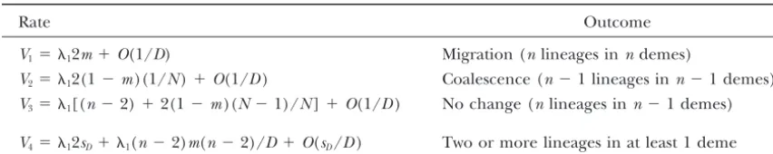
TABLE 2
The 27 distinguishable type␦and type 2 birth/death events in the history ofnlineages currently inn⫺1 different demes, grouped into just four kinds of events
Rate Outcome
V1⫽ 12m⫹O(1/D) Migration (nlineages inndemes)
V2⫽ 12(1⫺m)(1/N)⫹O(1/D) Coalescence (n⫺1 lineages inn⫺1 demes) V3⫽ 1[(n⫺2)⫹2(1⫺m)(N⫺1)/N]⫹O(1/D) No change (nlineages inn⫺1 demes)
V4⫽ 12sD⫹ 1(n⫺2)m(n⫺2)/D⫹O(sD/D) Two or more lineages in at least 1 deme
rate events that affect the sample configuration are of U*
7 ⫹P2(mig)U*6 ⫽ n
2
, (18)
O(1/D).
Thus, in a relatively short time, a sample ofnlineages
respectively. Therefore, the rates of coalescence and
in n ⫺ 1 demes will be converted to a sample of k
branching in the limiting (D → ∞) ancestral process
lineages inkdemes. The value ofkdepends on whether
become identical to the rates of coalescence and a coalescent event or a migration event occurs. If it is
branching in a panmictic ancestral selection graph, but a coalescent event, thenk⫽n⫺1, and if it is a migration
where time is measured in units of1generations. From
event, then k⫽ n. On the timescale above, with 1 ⫽
Equations 3 and 15 we can write1⫽ND/(2P2(mig)).
ND[1⫹(1⫺m)/(Nm)]/2, these events become
instan-Since we assume that 0⬍ mⱕ 1 andN ⱖ 1, we have
taneous because their rates approach infinity in the limit
0⬍P2(mig)ⱕ1 and1ⱖND/2. With a migration rate
D→∞. The result is an instantaneous adjustment that
of m ⫽ 1, the present model reduces to a panmictic
has two possible outcomes, with probabilities
model with timescale1⫽ND/2. Otherwise, the effect
of island-model subdivision is to lengthen the timescale P2(mig)⫽lim
D→∞ V1
V1⫹V2
⫽ Nm
Nm ⫹1⫺m (15) of the ancestral (and the forward-time) process.
Note that the processes of selection and mutation respond differently to subdivision. Mutation scales with and
1, while the selection parameter scales simply with
ND/2. In other words, there are different effective popu-P2(coal)⫽lim
D→∞ V2
V1⫹V2
⫽ 1⫺m
Nm⫹1⫺m. (16) lation sizes for selection and for mutation. The effective
size for selection is smaller and is equal toP2(mig)⫽
This will act as a filter on the four-rate Poisson process
Nm/(Nm⫹1⫺m) times the effective size for mutation.
described by Equations 9–12. Starting with the sample
The reason for this is that, when a branching event ofnlineages inndifferent demes, whenever a migration
creates a new lineage in the ancestral process, it has a event to an occupied deme occurs without immediate
P2(coal) ⫽ (1 ⫺ m)/(Nm ⫹ 1 ⫺ m) chance of being
coalescence (event 4), there is a chanceP2(mig) that erased by a coalescent event, so onlyP
2(mig) of them
the sample will be returned to its original state. The
are observable. In the present model, this cancels, ex-rest of the time,i.e., with probability P2(coal), event 4 is actly, the factor 1/P
2(mig) by which the number of
converted to event 3, which is a coalescent event.
When-branching events that occur in the limiting process is ever a branching event occurs where both parents stay
increased relative to the number under panmixia. For
in the same deme (event 6), there is a chanceP2(coal) the same reason, there is also a difference between the
that it is converted into self-collision, so that the sample
scalings for recombination, which splits lineages, and returns to its original state, and a chanceP2(mig) that it
mutation in similarly structured populations (
Nord-is converted into an observable branching event (event 7).
borg2000;LessardandWakeley2004).
It is straightforward to show that a Poisson process
The scattering phase:The results obtained above ap-filtered in this way is equivalent to a Poisson process
ply to the history of a sample ofnlineages inndifferent with an adjusted rate; for example, seeWakeley(1999).
demes. They follow from the fact that coalescent events
Thus, the probabilitiesP2(mig) andP2(coal) narrow the within multiply occupied demes and migration events
relevant number ofO(1/D) events to just two. Using
from multiply occupied demes to unoccupied demes Equations 9–12, and simplifying, the limiting rates of
occur with rates that areDtimes larger than the rates coalescence and branching become
of branching events and migration events to occupied demes. Because of this, whenever multiple samples are U*3 ⫹ P2(coal)U*4 ⫽
冢
n
2
冣
(17) taken from one or more demes, there will be a briefing-phase results above apply. The number of lineages with each remaining lineage in a separate deme,E[Y|n⬘] is the expected value ofY for a sample of size |n⬘| in our that remain at the end of the scattering phase, and that
then enter the collecting phase, will depend on the rescaled, unstructured, collecting-phase ASG. Below, we
use the framework of Equation 21 both analytically and number of coalescent events that occur within the
multi-ply sampled deme or demes. In the limit asD→∞, the in simulations, where our results are also consistent with keeping track of allelic configurations during the scat-duration of the scattering phase becomes negligible so
that it can be treated as instantaneous when time is tering phase.
A compression of the Markov process that describes
measured in proportion toDgenerations.
Because we have assumed thatsDisO(1/D), whereas the conditional evolution of the unstructured ASG is
found. This continuous-time Markov jump chain is an the rates of within-deme coalescence and migration to
occupied demes depend only onN,m, and the sample extension of the conditional ancestral selection graph
ofSlade (2000a) and is derived with new clarity. The size(s), the scattering phase here is the same as that in
a population in which all genetic variation is selectively result is a maximal compression of the ancestral selec-tion graph in which the timing properties of the graph equivalent. As inWakeley(1998), the scattering phase
for a sample of sizenall from a single deme is equivalent are retained. This continues, and improves upon, a
sim-ilar enhancement of the conditional graph by Slade
to a series of n Bernoulli trials with probabilities of
success (2000b) that reduces its branching rate. This is an
alter-native version of the minimal representation of the
con-ditional graph as discussed in Slade and Neuhauser
Pk(mig)⫽ ᏹ
ᏹ ⫹k⫺ 1, (19) (2003). Without the timing structure of the graph in
place, results that describe some probabilistic properties
for k⫽ 1, 2, . . . ,n, and in whichᏹ ⫽ Nm/(1 ⫺ m).
of a single ancestral lineage within the ASG are obtained Note that k⫽ 2 yields P2(mig) given in Equation 15.
byFearnhead(2002). The details of our general deriva-Success is defined to be the migration of one of the
tion are deferred toappendix b. lineages to an unoccupied deme, and each of these
The simulations presented inresultsare performed
increases by one the number of lineages that will enter
using the corresponding adaptation of a computational the collecting phase. If we usen⬘to denote the number
Monte Carlo method as in Slade(2000a,b). The
pur-of lineages that will enter the collecting phase, then
pose of such a simulation scheme is the calculation of an approximate probability distribution over the realiza-P[n⬘|n]⫽|S
(n⬘) n |ᏹn⬘
ᏹ(n)
(20)
tions of the genealogy. For a particular genealogy then, a weight is attributed to its associated time to the most
is its probability function (Wakeley 1998), in which
recent common ancestor (TMRCA), and the weighted
aver-the |Sn(n⬘)| are unsigned Stirling numbers of the first kind
age is evaluated upon completion of a large number of and ᏹ(n)⫽ ᏹ(ᏹ ⫹ 1) · · · (ᏹ ⫹ n ⫺ 1). Finally, the
repetitions. The improved efficiency in having attained scattering phase occurs independently among demes, so
the maximal compression of the genealogical Markov that we can multiply the probabilities (20) over samples
chain is substantial; running time until convergence from different demes.
that was previously required is now at least fully halved. The feasibility of at least doubling the branching and
METHODOLOGY mutation rates is also achieved. The performance gets better still when calculating statistics of theTMRCA
distri-We have shown that the ancestry of a sample from a
bution, as it would also do for properties of subtrees of subdivided population, with equal deme sizes and
is-the genealogy. Our compression reduces is-the number of land-type migration, and in which two alleles are subject
possible transitions required to describe the conditional to selection and mutation, includes an instantaneous
ASG at any event, from 10 to only 6. Thus, the size of scattering phase and then enters a collecting phase,
the state space of a realization of the conditional graph which is equivalent to the unstructured ASG with
muta-decreases exponentially. Hence, variance of any corre-tion and seleccorre-tion parameters scaled appropriately. This
sponding simulation technique is reduced. Depending means that ifYis any measurement on the sample, such
on the parameter combinations, to produce the com-as the time to common ancestry or the total length
posite PDFs inresultswith a Pentium 3.06GHz Xeon
of the genealogy, we can compute properties of Y by
processor, computing time ranged from a few hours to conditioning on the outcome of the scattering phase.
several days. For example, if E[Y|n] is the expected value of Yfor
the samplen⫽(n1, . . . ,nd) of size |n|⫽兺di⫽1ni fromd
different demes, then RESULTS
E[Y|n]⫽
兺
n⬘
E[Y|n⬘]P[n⬘|n], (21) From Equation 21 we can see that simple estimators
of the migration parameterᏹare as usefull when weak
selection is present as they are when all variation is where P[n⬘|n] is the product of probabilities like (20)
of identity in state for samples of size two taken from the collecting phase. Low migration rates yield sample figurations at the start of the collecting phase that con-same deme and from two different demes, respectively.
Taking the scattering phase into account, we have sist of close tod A1alleles andd A2alleles, provided all
of theddemes initially sampled contained at least one of each allele. The highest sensitivity to selection there-1⫺ q0⫽
ᏹ
ᏹ⫹1(1⫺q1), (22) fore is achieved when the population is structured
be-tween very many demes connected by an exceedingly and ifqˆ0 and qˆ1 are estimates of q0 and q1 from some
low migration rate. Note that this effect is independent data, then
of whether the initial sample contains mostly the favored or the unfavored allele.
ᏹ典 ⫽
冤
11⫺⫺qˆqˆ10
⫺1
冥
⫺1(23) To convert a coalescent time unit into years, it is
nec-essary to calculate the product of the (estimated)
effec-is an estimate ofᏹ. Note that (23) has the same form tive population size and number of years per
repro-as the various estimators of gene flow brepro-ased onFSTor pair- ductive generation. When the migration rateᏹⰆ1 we
wise sequence differences under the assumption of selec- compare the structured model only since according to
tive neutrality; see, for example,Hudsonet al.(1992). the factor calculated intheory, 1⫹ᏹ⫺1, a coalescent
Neither the unstructured ASG nor our slightly more time unit in the unstructured ASG represents
incompa-complicated structured ASG lends itself to analytical rably fewer numbers of generations. On the other hand,
computations much more involved than the above. whenᏹⰇ1 there is a meaningful comparison between
From Equation 21 it is clear how analysis of our struc- results with and without very many demes. Whenᏹ⫽
tured ASG is related to analysis of the unstructured 0.01 in the structured genealogies (both neutral and
graph. So, for example, it is possible to average such ex- selected) every generation that elapses according to
coa-pressions asKroneandNeuhauser’s(1997) Equation lescent time translates as 100 additional generations
3.5 for the expected time to the ultimate ancestor of in an unstructured genealogy. Population subdivision
the sample overn ⫽ |n⬘| at the start of the collecting magnifies the extent of changes to coalescence times
phase. Instead of this, we have used simulations that and thus immediately accentuates the effect of selection
include the scattering phase and the maximal compres- on genealogical time depth.
sion of the ASG described inappendix b to compute The interaction between migration and selection as
the probability density function of the time to the most it affects the distribution of the conditional TMRCA is
recent common ancestor of a sample (TMRCA). shown in Figures 2 and 3. The mutation rate is set at
In unstructured nonneutral genealogies with small three levels, ⫽0.01, 0.1, and 1. Low mutation rates
mutation rates certain sample configurations, among a are appropriate since we consider alleles corresponding
sample of sizen, have reduced mean coalescent times to amino acid replacements at a hypothetical nucleotide
when compared to their neutral counterparts, and other site within a single locus. (We note that ⫽0.001 yields
sample configurations have enlarged coalescent times a distribution of theTMRCAunder neutrality that is
ex-(Slade 2000a; see alsoSlade and Neuhauser2003). tremely similar to that obtained for ⫽ 0.01.) The
The mixtures of reduced sample configurations at the selection rate in our three cases is chosen in accordance
start of the collecting phase in the structured model with the weighted average predicted to be operating at
result in novel distributions of theTMRCAunder selection. nucleotide sites bySawyeret. al(2003), namely ⫽5
This mixture is the same under neutrality as it is with and 7.5. The migration rate is set to two levels, ᏹ ⫽
selection. The effect of the scattering phase under neu- 0.01 in Figure 2 andᏹ⫽ 10 in Figure 3.
trality is governed by the level of mutation in the collect- The probability density function (PDF) for the low
ing phase. Although the sample size is reduced, it can migration rate and low mutation rate case is presented
easily correspond to an increasedTMRCAbecause the ad- in Figure 2A. A substantial change in the shape of the
justed sample configuration requires longer to assimi- PDF is clear under selection. Increasing the mutation
late its ancestors (particularly for low mutation rates). rate, the next lowest migration rate case is shown Fig-In the unstructured ASG as the mutation rate decreases ure 2B. The extent of the effect of selection appears to
the conditional genealogy becomes more sensitive to diminish at our highest level of the mutation rate in
the presence of selection (Slade2000a). However, the Figure 2C. The parameters (mean and standard
devia-sample configurations that yield the greatest selective tion) of these distributions are compared in Table 3.
effect are also the samples least likely to be obtained, In the last case just mentioned, we have a particularly
having extremely small sampling probabilities. The sam- novel result as the mean starts to increase again, i.e.,
pling distribution is increasingly U-shaped as de- toward neutrality, with the selection strength above
creases, and under selection, samples dominated by the some threshold. In both Figure 2 and Table 3 it is
as-favored allele are more likely than those dominated by sumed that samples of size 12 were taken from each of
the unfavored allele. Introducing population subdivi- four demes, and that each of the four samples included
sion makes the most sensitive samples accessible because one copy of alleleA1and 11 copies of alleleA2, or (1, 11)
Figure3.—PDFs for theTMRCAof a sample of size 48 spread
evenly among four demes, but comparing two sample distribu-tions of allelesA1andA2: (1, 11) as in Figure 2 and (11, 1).
In all cases,ᏹ ⫽10 and ⫽ 0.1. As in Figure 2, the solid curve shows the PDF for ⫽ 0; the long-dashed curves, for
⫽5.0; and the short-dashed curves, for ⫽7.5.
(11, 1), respectively. The effect on the shape of the PDFs can be discerned; however, in Table 4 comparisons of the parameters of the distributions under panmixia
are also shown. With a migration rate as high asᏹ ⫽
10, the effects of many-demes population structure in Table 4, for both neutral and selected genealogies, can still be distinguished. In the neutral case (Table 4, left column), even with the sample size adjustment the mean
Figure2.—PDFs for theTMRCAof a sample of size 48 spread TMRCA is considerably higher than it is for panmixia.
evenly among four demes and with sample allele counts (1A1, Comparing the two rows of Table 4, we can see that this
11A2). A–C depict results for three different mutation rates
also reflects the 10% lengthening of the genealogies
as indicated. The migration parameter wasᏹ⫽0.01, and the
expected whenᏹ⫽10. The difference in the selective
solid curve shows the PDF for ⫽0; the long-dashed curves,
effect between the two completely different initial
sam-for ⫽5.0; and the short-dashed curves, for ⫽7.5. The
case of ⫽0.01 and ⫽7.5 could not be completed due to ples is only minor. prohibitive computational requirements.
DISCUSSION
In contrast, when the migration rate is high the
sam-ple size adjustment is moderate, and the initial samsam-ple We have obtained a simple structured ancestral
selec-tion graph in the limit as the number of demes tends configurations show very similar responses to selection.
The PDFs shown in Figure 3, A and B, correspond to to infinity and with island-type migration among demes
of equal size. The result is understood as an approxima-different initial samples within each deme of being
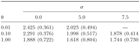
TABLE 3 model (Wakeley 1998). In other words, migration structures selected variation within and between demes The means and the standard deviations (in parentheses)
in a way that is identical to the way it structures neutral of the PDFs depicted in Figure 2
variation. This can be seen as a consequence of the fact
that the model applies to 0⬍ m ⱕ 1 whilesD → 0 as
D → ∞, so that migration is stronger than selection
0.0 5.0 7.5
within demes. However, using the improved algorithm
0.01 2.425 (0.361) 2.023 (0.494) — for simulation of selected genealogies conditional on
0.10 2.291 (0.376) 1.998 (0.517) 1.878 (0.414) the frequencies ofA1andA2in the sample, we have also 1.00 1.888 (0.722) 1.618 (0.804) 1.744 (0.730) shown a strong effect of migration on theT
MRCAof some
samples. Namely, limited migration can convert even very unbalanced samples into balanced ones,e.g., (1, 11)→
of weak selection from populations composed of a large (1, 1), and place the collecting-phase ancestral sample
number of demes. Convergence to the simpler process into the range of samples for which theTMRCAis reduced
occurs due to the difference in timescales between mi- by selection. This happens because there are no
muta-gration and drift within demes on the one hand and se- tions during the scattering phase, while coalescent
lection and mutation across the entire population on the events between like alleles can occur. However, we note
other. Under neutrality, results of this sort can be proven that although unbalanced samples, like (1, 11), within
using the technique developed byMo¨ hle(1998a,b) for demes are more likely to be obtained than balanced
calculating the transition rates of (ancestral) Markov samples, like (6, 6), when the migration rate is small it
processes with a separation of timescales. For ancestries will be even more typical for single-deme samples to be
under weak selection, the framework of birth-death pro- fixed for one allele or the other. This can be seen in
cesses is more appropriate because the addition of new Equation 1, which converges to0⫽ 1⫺xandN⫽x
lineages at type 2 branching events increases the dimen- in the limitm→ 0.
sionality that would be required in Mo¨hle’s analysis. We We note also that if we had not assumed the mutation
have shown that one can truncate the system by ignoring rate to be small (uD → 0 as D → ∞), we would have
the transitions of very small rates to obtain a closed obtained a neutral limiting graph. When the mutation
approximated system; we then found the correct transi- rate in the ancestral selection graph is infinite the
tion rates in the limiting process were provided by the branching-coalescing structure collapses to a neutral
corresponding calculation. coalescent process (Neuhauser and Krone 1997).
Our analysis does not provide an estimate of the error Allowing mutation in the scattering phase of the
struc-incurred in applying the limiting model to real (i.e., tured ancestral selection graph also yields a neutral (coa-finite) populations. One way to address this is using sim- lescent) ancestral process, since this would render an
ulations, such as those reported inLessardandWakeley infinite mutation rate in the collecting phase. That is,
(2004). In that article, simulations demonstrated the if the mutation probabilityisO(1) instead ofO(1/D)
rapid convergence of the distribution of the total length then mutation is a fast timescale event and will occur
of the gene genealogy of a sample of size two to that in the scattering phase amid the rapid migration and
predicted by the limiting (D→∞) ancestral recombina- coalescent events also ofO(1). Whenever the process
tion graph with island model migration among demes. switches over to the slower transitions, such as those in
Populations composed of 100 or more demes were Table 1 that areO(1/D), mutation still occurs at a fast
closely approximated by the limiting model. rate and →∞, asD→∞.
It is clear that any quantity of interest can be com- We would like to clarify the case of zero mutation
puted using the framework of Equation 21, that is, by con- rate that leads to a neutral coalescent in the ASG. When
ditioning on the outcome of the scattering phase. In ⫽0, ancestors are always of one type only, but in the
fact, in the case of weak selection and mutation consid- dual process 2-arrows occur at a faster rate than␦-arrows. If all ancestors areA1 only the slower-rate␦-arrows are
ered here, there is a lot of parity with the strictly neutral
TABLE 4
Comparison of the means and the standard deviations (in parentheses) of theTMRCAin the unstructured ASG to those of the PDFs depicted in Figure 3 rescaled by
the factor 1⫹ᏹ⫺1so that they are measured in the same units
(1, 11)⫻4 demes (11, 1)⫻4 demes
⫽0 ⫽5 ⫽7.5 ⫽5 ⫽7.5
ᏹ⫽10 2.318 (0.432) 2.195 (0.408) 2.173 (0.377) 2.271 (0.889) 2.165 (0.752)
Kaplan, N. L., R. R. HudsonandC. H. Langley, 1989 The
“hitch-needed to describe the ancestral process since 2-arrows
hiking effect” revisited. Genetics123:887–899.
are never followed, and this yields the neutral coales- Karlin, S., andH. M. Taylor, 1975 A First Course in Stochastic
Pro-cesses. Academic Press, New York.
cent. On the other hand, having allA2ancestors both
Kimura, M., 1955 Stochastic processes and the distribution of gene
the ␦-arrows and the faster-rate 2-arrows participate in
frequencies under natural selection. Cold Spring Harbor Symp.
the ancestral process. However, the outcome of 2-arrows Quant. Biol.20:33–53.
Kimura, M., 1983 The Neutral Theory of Molecular Evolution.
Cam-is determined in thCam-is case; they will always be followed
bridge University Press, Cambridge, MA.
and no uncertainty arises in the path taken by the dual
Kingman, J. F. C., 1982a The coalescent. Stoch. Proc. Appl.13:235–248.
process of a sample. No virtual ancestors are needed and Kingman, J. F. C., 1982b Exchangeability and the evolution of large
populations, pp. 97–112 inExchangeability in Probability and
Sta-when a branching event occurs in the Markov process
tistics, edited by G.Kochand F.Spizzichino. North-Holland,
corresponding to the conditional ASG, it represents a
Amsterdam.
so-called null transition, as discussed in appendix b. Krone, S. M., andC. Neuhauser, 1997 Ancestral processes with selection. Theor. Popul. Biol.51:210–237.
Recalculating the Markov process without these
transi-Lessard, S., andJ. Wakeley, 2004 The two-locus ancestral graph
tions yields the same neutral coalescent as required.
in a subdivided population: convergence as the number of demes grows in the island model. J. Math. Biol.48:275–292. We thank both referees for their reports. P.F.S. thanks the Wakeley
Mo¨ hle, M., 1998a Coalescent results for two-sex population models. Lab and the Department of Organismic and Evolutionary Biology at
Adv. Appl. Probab.30:513–520. Harvard for their hospitality during a visit. J.W. was supported by a
Mo¨ hle, M., 1998b A convergence theorem for Markov chains arising Presidential Early Career Award for Scientists and Engineers from
in population genetics and the coalescent with partial selfing. the National Science Foundation (DEB-0133760). P.F.S. was also sup- Adv. Appl. Probab.30:493–512.
ported by a travel fund from the Faculty of Science at the University of Mo¨ hle, M., 1998c Robustness results for the coalescent. J. Appl. Sydney. This is research publication no. 0009 from Sydney University Probab.35:438–447.
Bioinformatics and Technology Centre. Moran, P. A. P., 1958 Random processes in genetics. Proc. Camb. Philos. Soc.54:60–71.
Moran, P. A. P., 1962 Statistical Processes of Evolutionary Theory. Clar-endon Press, Oxford.
Nath, H. B., and R. C. Griffiths, 1996 Estimation in an island LITERATURE CITED
model using simulation. Theor. Popul. Biol.50:227–253. Aldous, D. J., 1985 Exchangeability and related topics, pp. 1–198 Neuhauser, C, 1999 The ancestral graph and gene genealogy under
inE´cole d’E´te´ de Probabilite´s de Saint-Flour XII–1983(Lecture Notes frequency-dependent selection. Theor. Popul. Biol.56:203–214. in Mathematics, Vol. 1117), edited by A.Doldand B.Eckmann. Neuhauser, C., andS. M. Krone, 1997 The genealogy of samples Springer-Verlag, Berlin. in models with selection. Genetics145:519–534.
Avise, J. C., 2000 Phylogeography: The History and Formation of Species. Nordborg, M., 2000 Linkage disequilibrium, gene trees and selfing: Harvard University Press, Cambridge, MA. an ancestral recombination graph with partial selfing. Genetics Bahlo, M., andR. C. Griffiths, 2000 Inference from gene trees 154:923–929.
in a subdivided population. Theor. Popul. Biol.57:79–95. Notohara, M., 1990 The coalescent and the genealogical process Barton, N. H., A. M. EtheridgeandA. K. Sturm, 2004 Coalescence in geographically structured population. J. Math. Biol.29:59–75. in a random background. Ann. Appl. Probab.14:754–785. Ohta, T., andM. Kimura, 1971 On the constancy of the evolution-Beerli, P., andJ. Felsenstein, 1999 Maximum-likelihood estima- ary rate of cistrons. J. Mol. Evol.1:18–25.
tion of migration rates and effective population numbers in two Sawyer, S. A., andD. L. Hartl, 1992 Population genetics of poly-populations using a coalescent approach. Genetics152:763–773. morphism and divergence. Genetics132:1161–1176.
Beerli, P., andJ. Felsenstein, 2001 Maximum-likelihood estima- Sawyer, S. A., R. J. Kulathinal, C. D. BustamanteandD. L. Hartl, tion of a migration matrix and effective population sizes innpop- 2003 Bayesian analysis suggests that most amino acid replace-ulations by using a coalescent approach. Proc. Natl. Acad. Sci. ments inDrosophilaare driven by positive selection. J. Mol. Evol.
USA98:4563–4568. 57:S154–S164.
Bustamante, C. D., R. Nielsen, S. A. Sawyer, K. M. Olsen, M. D. Slade, P. F., 2000a Simulation of selected genealogies. Theor. Po-Puruggananet al., 2002 The cost of inbreeding inArabidopsis. pul. Biol.57:35–49.
Nature416:531–534. Slade, P. F., 2000b Most recent common ancestor probability distri-De Iorio, M., andR. C. Griffiths, 2004 Importance sampling on butions in gene genealogies under selection. Theor. Popul. Biol.
coalescent histories. ii. subdivided population models. Adv. Appl. 58:291–305.
Probab.36:434–454. Slade, P. F., andC. Neuhauser, 2003 Nonneutral genealogical Ethier, S. N., andT. Nagylaki, 1980 Diffusion approximations of structure and algorithmic enhancements of the ancestral selec-Markov chains with two timescales and applications to population tion graph. Theor. Biol.8:255–278 (erratum: Theor. Biol.8:539). genetics. Adv. Appl. Probab.12:14–49. Slatkin, M., 1985 Gene flow in natural populations. Annu. Rev.
Ecol. Syst.16:393–430. Fearnhead, P., 2002 The common ancestor at a nonneutral locus.
J. Appl. Probab.39:38–54. Slatkin, M., 1987 The average number of sites separating DNA sequences drawn from a subdivided population. Theor. Popul. Golding, B., 1994 Non-Neutral Evolution. Chapman & Hall, New York.
Griffiths, R. C., 1991 The two-locus ancestral graph, pp. 100–117 Biol.32:42–49.
Stephens, M., 2001 Inferences under the coalescent, pp. 213–238 inSelected Proceeedings of the Symposium on Applied Probability, edited
by I. V.Basawaand R. L.Taylor. Institute of Mathematical Sta- inHandbook of Statistical Genetics, edited by D. J.Balding, M. J. Bishopand C.Cannings. John Wiley & Sons, Chichester, En-tistics, Hayward, CA.
Hey, J., andC. A. Machado, 2003 The study of structured popula- gland.
Stephens, M., andP. Donnelly, 2003 Ancestral inference in popula-tions—new hope for a difficult and divided science. Nat. Rev.
Genet.4:535–543. tion genetics models with selection. Aust. N. Z. J. Stat.45:395–430. Strobeck, C., 1987 Average number of nucleotide differences in a Hudson, R. R., 1983 Testing the constant-rate neutral allele model
with protein sequence data. Evolution37:203–217. sample from a single subpopulation: a test for population subdivi-sion. Genetics117:149–153.
Hudson, R. R., M. SlatkinandW. P. Maddison, 1992 Estimation
of levels of gene flow from DNA sequence data. Genetics132: Tajima, F., 1983 Evolutionary relationship of DNA sequences in finite populations. Genetics105:437–460.
583–589.