Optimal Design for Minimizing Uncertainty in Dynamic Equilibrium Systems

(1)

Optimal Design for Minimizing Uncertainty in Dynamic Equilibrium

Systems

H.T. Banks, Robert Baraldi, Kevin Flores

Department of Mathematics

Center for Research in Scientific Computation

North Carolina State University

Raleigh, NC

March 7, 2015

Abstract

We further develop and utilize a previously described optimal design framework to investigate an oscillatory system of 16 states which simulates the circadian rhythm and intertwined positive and negative regulatory loops ofPer,Cry,Bmal1, andClock genes in mammals. We illustrate use of a subset selection methodology with experimental perturbations in order to increase and possibly maximize the amount of information gained from longitudinal data derived from such experiments. We demonstrate that optimizing experimental perturbations may substantially decrease uncertainty in estimating model parameters.

(2)

1 Introduction

Current efforts in modeling the host immune response to HIV infection and RNA3 recruitment in the Brome Mosiac Virus (BMV) replication cycle have elucidated the relationship between disturbances that drive biological systems away from equilibrium and information content in such perturbations [2, 1]. For instance, the BMV model developed by Banks, et al. [4, 1] describes how experimental input manipulation can produce non-equilibrium system dynamics, which leads to a greater information content in collected data. The findings in [1] suggest that input manipulation is a powerful tool for reducing standard errors in parameter estimates. In the HIV model developed by Banks, et al. [2], anti-retroviral therapy (ART) drives viral load in patients toward an equilibrium level that is undetectable by ultra-sensitive assays. When ART is interrupted, often due to patient negligence, the HIV model converges to an equilibrium with high viral load. One of the results of [2] was that as the authors fit the HIV model to clinical patient data, the number of HIV model parameters that could be easily estimated with high statistical confidence increased with the number of treatment interruptions. Thus, non-equilibrium dynamics induced by ART perturbations increased the data information content as calculated through asymptotic standard errors for estimated model parameters.

In this paper, we look at the effects on parameter estimation that results from perturbing a dynamic system away from its oscillatory steady state. We hypothesize that disturbing an oscillatory system away from equilibrium yields better information for parameter estimation than an unaltered or undisturbed system, as evidenced by providing more statistical certainty in parameters for the model. To investigate this, we analyzed a mathematical model describing the regulation of genes involved in mammalian circadian rhythms. The expression of these genes can be inhibited through silencing their respective mRNAs. This permits the researcher to effectively negate the expression of a certain gene, thereby perturbing the system away from its periodic equilibrium. We employed an optimal experimental design theory framework described in [1], and further developed the algorithm to minimize parameter standard errors by choosing optimal times to perturb the model away from its dynamic equilibrium. Variations on the observation frequency and length of experiment are analyzed in the context of this algorithm, as well as the number of possible perturbations allowed. We report how optimization of experimentally controlled inputs, i.e., RNA inhibition (RNAi), for the circadian system can lead to a substantial decrease in standard errors for model parameters, thereby increasing the levels of certainty in parameters for the model.

2 Mathematical model

2.1 Circadian rythms model

The mathematical model of circadian rythms we used was previously developed in [9]; it is an oscillatory system of 16 state variables desribing a regulatory network of thePer,Cry,Bmal1, andClock genes in mammals. Of the four parameter sets presented in [9], parameter set 1 of the model, described in Tables 1 and 2 of this paper and Table 2 of [9], models the protein and mRNA levels of the aforementioned genes in continuous darkness, which gives rise to the desired sustained circadian oscillations. The mechanism of circadian oscillation relies on the for-mation of an inactive complex between PER and CRY and the activators CLOCK and BMAL1 that enhancePer

andCry expression [9]. The occurence and period of these oscillations are generally most sensitive to parameters related to synthesis or degradation ofBmal1 mRNA or BMAL1 protein. The developers of this model concluded that sustained oscillations might arise from the sole negative autoregulation of Bmal1 expression. When the researchers integrated light-induced expression of thePer gene, the model accounted for rhythmic regulation of the oscillations by the light-dark cycle. Given the sustained oscillations of the model at steady state as well as the large number of system parameters, we found the model appropriate for assessing the impact of perturbing an oscillatory system away from the dynamic equilibrium on the uncertainty associated with estimating model pa-rameters. The equations have been grouped by mRNAs, the phosphorylated and non-phosphorylated PER-CRY complex in the cytosol and nucleus, the phosphorylated and non-phosphorylated protein BMAL1 in the cytosol and nucleus, and the complex between PER-CRY and CLOCK-BMAL1 in the nucleus. The model, as developed in [9], is as follows:

(3)

dMP

dt =vsP Bn

N

Kn AP+BnN

−vmP

MP

KmP +MP

−kdmpMP, (1)

dMC

dt =vsC Bn

N

Kn AC+BNn

−vmC

MC

KmC+MC

−kdmcMC, (2)

dMB

dt =vsB Km

IB

Km IB+BNm

−vmB

MB

KmB+MB

−kdmbMB. (3)

(b) Phosphorylated and non-phosphorylated proteins PER and CRY in the cytosol:

dPC

dt =ksPMP−V1P PC

KP+PC +V2P

PCP

Kdp+PCP

+k4P CC−k3PCCC−kdnPC, (4)

dCC

dt =ksCMC−V1C CC

KP+CC +V2C

CCP

Kdp+CCP

+k4P CC−k3PCCC−kdcCC, (5)

dPCP

dt =V1P PC

KP +PC

−V2P

PCP

Kdp+PCP

−vdP C

PCP

Kd+PCP

−kdnPCP, (6)

dCCP

dt =V1C CC

KP+CC

−V2C

CCP

Kdp+CCP

−vdCC

CCP

Kd+CCP

−kdnCCP. (7)

(c) Phosphorylated and non-phosphorylated PER-CRY complex in the cytosol and nucleus:

dP CC

dt =−V1P C

P CC

KP +P CC

+V2P C

P CCP

Kdp+P CCP

−k4P CC+k3PCCC+k2P CN−k1P CC−kdnP CC, (8)

dP CN

dt =−V3P C

P CN

KP +P CN

+V4P C

P CN P

Kdp+P CN P

−k2P CN +k1P CC−k7BNP CN +k8IN−kdnP CN, (9)

dP CCP

dt =V1P C

P CC

KP+P CC

−V2P C

P CCP

Kdp+P CCP

+−vdP CC

P CCP

KD+P CCP

−kdnP CCP, (10)

dP CNP

dt =V3P C

P CV

KP+P CV

−V4P C

P CN P

Kdp+P CN P

+−vdP N C

P CN P

KD+P CN P

−kdnP CN P. (11)

(d) Phosphorylated and non-phosphorylated protein BMAL1 in the cytosol and nucleus:

dBC

dt =ksBMB−V1B BC

KP+BC +V2B

BCP

Kdp+BCP

(4)

dBCP

dt =V1B BC

KP +BC

−V2B

BCP

Kdp+BCP

−vdBC

BCP

Kd+BCP

−kdnBCP, (13)

dBN

dt =−V3B BN

KP+BN +V4B

BN P

Kdp+BN P

+k5BC−k6BN−k7BNP CN+k8IN −kdnBN, (14)

dBN P

dt =V3B BN

KP+BN

−V4B

BN P

Kdp+BN P

−vdBN

BN P

Kd+BN P

−kdnBN P. (15)

(e) Inactive complex between PER-CRY and CLOCK-BMAL1 in the nucleus:

dIN

dt =−k8IN+k7BNP CN−vdIN IN

Kd+IN

−kdnIN. (16)

Definitions of all the parameters used in these equations are in Tables 1 and 2. In Equations (1)-(16), concentrations are defined with respect to total cell volume. The initial conditions for this system are IC =

{0,0,8.7,0,0,0,0,0,0,0,0,0,0,0,0,0}; all are zero except the amount of Bmal1 mRNA. The concentration of every protein species (single or complex) is denoted by a subscript C, N, CP, or N P for the cytosolic, nuclear, cytosolic phsophorylated or nuclear phosphorylated form, respectively.

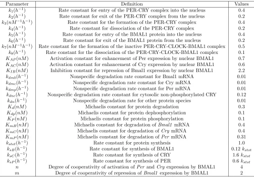
Due to the substantial number of parameters present in the model and the combinatorial nature of the pa-rameter subset selection method detailed in Section 4, we first had to reduce the number of papa-rameters that were assumed to be estimated. In [9], the authors state that many parameter values remain to be determined experimentally, and that the oscillations created were obtained for a semi-arbitrary choice of parameter val-ues in a physiologically realistic range. Given the somewhat arbitrariness of the parameter valval-ues and the implied difficulty of experimental estimation, we selected parameters based on mathematical type and biolog-ical significance. We also tried to select parameters that would represent a varying degree of sensitivity, and gathered this sensitivity information based on the values in Table 2 of [9]. Parameters k1 through k8 are all

rate constants for the protein complexes described in the model, and act as decay or growth rates. Parame-ters KAP, KAC, and KIB describe the activation or inhibition of mRNA’s by nuclear BMAL1, and appear in the model as Michaelis-Menten constants. Parameters Kd, Kdp, KP, KmB, KmC and KmP are all Michaelis-Menten constants for proteins and mRNA’s, and describe either degradation or phosphorylation processes. The parameter set that we apply the subset selection algorithm, developed in [3] and employed in [2, 1], is

(5)

Parameter Definition Values

k1(h−1) Rate constant for entry of the PER-CRY complex into the nucleus 0.4

k2(h−1) Rate constant for exit of the PER-CRY complex from the nucleus 0.2

k3(nM−1h−1) Rate constant for the formation of the PER-CRY complex 0.4

k4(h−1) Rate constant for dissociation of the PER-CRY complex 0.2

k5(h−1) Rate constant for entry of the BMAL1 protein into the nucleus 0.4

k6(h−1) Rate constant for exit of the BMAL1 protein from the nucleus 0.2

k7(nM−1h−1) Rate constant for the formation of the inactive PER-CRY-CLOCK-BMAL1 complex 0.5

k8(h−1) Rate constant for the dissociation of the PER-CRY-CLOCK-BMAL1 complex 0.1

KAP(nM) Activation constant for enhancement of Per expression by nuclear BMAL1 0.7

KAC(nM) Activation constant for enhancement of Cry expression by nuclear BMAL1 0.6

KIB(nM) Inhibition constant for repression of Bmal1 expression by nuclear BMAL1 2.2

kdmb(h−1) Nonspecific degradation rate constant for Bmal1 mRNA 0.01

kdmc(h−1) Nonspecific degradation rate constant for Cry mRNA 0.01

kdmp(h−1₎ _{Nonspecific degradation rate constant for Per mRNA} _0.01

kdnc(h−1₎ _{Nonspecific degradation rate constant for cytosolic non-phosphorylated CRY} _0.12

kdn(h−1₎ _{Nonspecific degradation rate for other protein species} _0.01

Kd(nM) Michaelis constant for protein degradation 0.3

Kdp(nM) Michaelis constant for protein dephosphorylation 0.1

KP(nM) Michaelis constant for protein phosphorylation 0.1

KmB(nM) Michaelis constant for degradation ofBmal1 mRNA 0.4

KmC(nM) Michaelis constant for degradation ofCry mRNA 0.4

KmP(nM) Michaelis constant for degradation of Per mRNA 0.31

kstot(h−1) Rate constant for protein synthesis 1.0

ksB(h−1) Rate constant for synthesis of BMAL1 0.12kstot

ksC(h−1) Rate constant for synthesis of CRY 1.6 kstot

ksP(h−1) Rate constant for synthesis of PER 0.6 kstot

n Degree of cooperativity of activation ofPer and Cry expression by BMAL1 4

m Degree of cooperativity of repression ofBmal1 expression by BMAL1 2

(6)

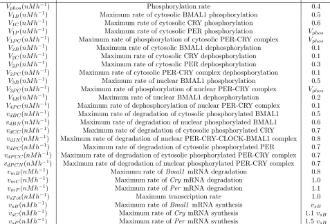
Parameter Definition Values

Vphos(nM h−1₎ _{Phosphorylation rate} _0.4

V1B(nM h−1) Maximum rate of cytosolic BMAL1 phosphorylation 0.5

V1C(nM h−1) Maximum rate of cytosolic CRY phosphorylation 0.6

V1P(nM h−1) Maximum rate of cytosolic PER phosphorylation Vphos

V1P C(nM h−1) Maximum rate of phosphorylation of cytosolic PER-CRY complex Vphos

V2B(nM h−1) Maximum rate of cytosolic BMAL1 dephosphorylation 0.1

V2C(nM h−1) Maximum rate of cytosolic CRY dephosphorylation 0.1

V2P(nM h−1) Maximum rate of cytosolic PER dephosphorylation 0.3

V2P C(nM h−1) Maximum rate of cytosolic PER-CRY complex dephosphorylation 0.1

V3B(nM h−1) Maximum rate of nuclear BMAL1 phosphorylation 0.5

V3P C(nM h−1) Maximum rate of phosphorylation of nuclear PER-CRY complex Vphos

V4B(nM h−1) Maximum rate of nuclear BMAL1 dephosphorylation 0.2

V4P C(nM h−1) Maximum rate of dephosphorylation of nuclear PER-CRY complex 0.1

vdBC(nM h−1) Maximum rate of degradation of cytosolic phosphorylated BMAL1 0.5

vdBN(nM h−1) Maximum rate of degradation of nuclear phosphorylated BMAL1 0.6

vdCC(nM h−1) Maximum rate of degradation of cytosolic phosphorylated CRY 0.7

vdIN(nM h−1₎ _{Maximum rate of degradation of nuclear PER-CRY-CLOCK-BMAL1 complex} _0.8

vdP C(nM h−1) Maximum rate of degradation of cytosolic phosphorylated PER 0.7

vdP CC(nM h−1) Maximum rate of degradation of cytosolic phosphorylated PER-CRY complex 0.7

vdP CN(nM h−1) Maximum rate of degradation of nuclear phosphorylated PER-CRY complex 0.7

vmB(nM h−1) Maximum rate ofBmal1 mRNA degradation 0.8

vmC(nM h−1) Maximum rate ofCry mRNA degradation 1.0

vmP(nM h−1) Maximum rate ofPer mRNA degradation 1.1

vsT ot(nM h−1) Maximum transcription rate 1.0

vsB(nM h−1) Maximum rate ofBmal1 mRNA synthesis vsB

vsC(nM h−1) Maximum rate ofCry mRNA synthesis 1.1vsB

(7)

2.2 Model for system perturbations using RNAi

We model the RNA inhibiter (RNAi) by introducing an additional state variable r that represents the con-centration of exogenously spawned small interfering RNAs (siRNA’s) that can inhibit a target mRNA post-transcriptionally. The intracellular concentration of siRNA is modeled by the equation

dr

dt =u(t)ron−rdr. (17)

The functionu(t) is a piecewise constant function with range in{0,1}that represents whether the RNAi is on or off for each ofH time intervals [tb

i−1, tbi],i= 1, . . . , H. The functionu(t) signifies whether the RNAi is active (= 1) or inactive (= 0) in certain intervals of time. The parameterronrepresents the rate of siRNA influx into cells andrd is the siRNA exponential decay rate. The constantrd was taken to be 2 hours−1as described in [11]. Due to the lack of literature on the value of ron, we assume it is equal to 4 (concentration/hour), as this represents a seemingly reasonable rate of siRNA influx. It is assumed there is initially no silencer in the system (r(0) = 0). To simulate the effect of RNAi in the model, we had the RNAi influence the removal rate of the Per mRNA.

The description of RNAi was inserted into Equation (1) by creating a (1 +mrr) term and multiplying it by the decay ratekdmpMP. Here,mr is the mass action interaction rate betweenrandMp. The modified equation forPer mRNA is now

dMp

dt =vsP Bn

N

Kn AP+BNn

−vmP

MP

KmP +MP

−kdmp(1 +mrr)MP, (18)

where mr is taken to be 10. It is important to note that while this may seem a high value, for simplification we did not want to affect more than one mRNA removal rate, and thus needed a slightly larger value to obtain a reasonable perturbation magnitude. Thus, we have implemented a state that will increase the rate at which

Per mRNA is removed, and in combination with the function u(t), effectively introduces perturbations into the system.

3 Optimal experimental design theory

3.1 Uncertainty quantification with asymptotic theory

We employed asymptotic theory in order to quantify parameter uncertainty within an optimal experimental design framework. Below, we formulate a Fisher Information Matrix, i.e., from asymptotic theory, for a given assumed level of observation noise and a function describing system perturbations, i.e., u(t). In the model above (specifically Equation (18)), the function u(t) is assumed to be known as it is controlled by the experimenter. With the addition of the RNAi, we can write the circadian model generally as

d~x

dt(t) =~g(t, ~x(t; ˆq, u(t)),q, uˆ (t)), t∈[t0, tf], ~

x(t0) =~x0, f~(t; ˆq, u(t)) =C~x(t; ˆq, u(t))

(19)

where~x0are given fixed initial conditions,~x(t; ˆq, u(t)) is the vector of state variables of the system time pointtand

parameter vector ˆq∈Rp, withp= 18 “estimated” parametersP from the total set of 55 model parameters from Tables 1 and 2. The initial time and final time are designatedt0andtf, respectively. LetP1([t0, tf]) denote the set of all bounded distributions on the interval [t0, tf]. The set of functions describing RNAi perturbations we use is

the set of piecewise constant functions with a domain [t0, tf] that is divided intoH intervals with variable length, and with a range in{0,1}. Specifically, letS={s= (s0, s1, . . . , sH)∈RH+1|si< si+1 fori= 0, . . . , H−1} and

letB =ZH

2. Then the perturbation function is defined in a piecewise constant fashion as u(t) :=u(t;b, s) =bi for t∈[si−1, si], i= 1, . . . , H, where b ∈B and s∈S. Thus the set U ≃B×S contains all of the admissible

perturbation functions u(t;b, s). LetP2(U) represent the set of all bounded distributions P2(u) onU. Then the

Generalized Fisher Information Matrix (GFIM) may be written

F(P1,P2,qˆ) =

Z tf

t0

Z

ZH

2

∇T

ˆ

qf~(t; ˆq, u(t)) V

−1

0 (t)

(8)

Here ˆq= ˆq0 is the assumed “true” parameter vector with the corresponding statistical error model (see Section

3.2.2 of [6]), which we assume to be constant, given by

~

Y(t) =f~(t; ˆq, u(t)) +Ee(t), (21)

where f~(t; ˆq, u(t))∈R6 and theEe(t) are independent and identically distributed with zero mean and covariance matrix given by V0(t).

We consider the case of observations collected at discrete times where we choose a set of n time points

τ ={tj},j = 1,2, . . . , n, and t0=t1< t2<· · ·< tn =tf. The corresponding discretep×pFisher information matrix (FIM) for a perturbation functionu(t;b, s) measured at discrete timesτ is

F(τ, u,qˆ) = n

X

j=1

∇T

ˆ

qf~(tj; ˆq, u(tj;b, s)) V0−1(tj)∇qˆf~(tj; ˆq, u(tj;b, s)). (22)

Here, V0 is taken to be the 6×6 diagonal matrix V0 = diag(σ2, ..., σ2) and we assume for these calculations

that the variance is equal to a constant value of σ2 = 1 for all states. The values in the sensitivity matrices

∇qˆf~(tj; ˆq, u(tj)) were calculated using the complex-step derivative method (see Section 3.2) and the parameters ˆ

qsupplied inP from those in Tables 1 and 2. Indeed, throughout we tacitly assume that these ˆq resulted from a prior best fit parameters to data. The choice of optimal design criteria is given by the minimization of a functional

J(F) : Rp×p _→ _R+_{; we utilize SE-optimal design, introduced in [5]. For any component} _q

k of the estimated parameter vector ˆq, the standard error (SEk) is computed by methods of asymptotic theory [7] that rely on the Fisher Information Matrix (Equation (22)).

3.2 Complex-step derivative method for calculating sensitivities

We briefly describe the complex-step derivative (see [10] for details) used to calculate an approximation for the sensitivities of the six species seen in Figure 2 of [9] with respect to model parameters. These species are: MP, the mRNA of Per; MC, the mRNA of Cry; MB, the mRNA of Bmal1; CT ot, the total amount of CRY; PT ot, the total amount of PER, and BT ot, the total amount of BMAL1. Essentially, the complex-step derivative is a finite-difference approximation calculated in the complex plane. Recall the forward-difference formula, wherein a common estimate for the first derivative of a scalar functionf(x) is

f′(x) =f(x+h)−f(x)

h +o(h), (23)

wherehis the finite-difference interval ando(h) is the truncation error for the first-order approximation. Consider a functionf =u+ivof the complex variablez=x+iy. Paraphrasing [10], iff is analytic in the complex plane then the Cauchy-Riemann equations apply and are given by

∂u ∂x =

∂v

∂y (24)

∂u ∂y =−

∂v

∂x. (25)

Equations (24) and (25) give the relationship between the real and imaginary parts of the function. We can use the definition of a derivative in the right hand side of the first Cauchy-Riemann Equation (24) to write

∂u ∂x = limh→0

v(x+i(y+h))−v(x+iy)

h , (26)

where his a real number. Since the Equations (1)-(16) are real functions of real variables, y = 0, u(x) =f(x), andv(x) = 0. Equation (26) can be rewritten as

∂f ∂x = limh→0

Im[f(x+ih)]

(9)

and approximated by

∂f ∂x ≈

Im[f(x+ih)]

h . (28)

The value of h is taken to be very small, e.g., h = 10−50_{. This is the} _{complex-step derivative approximation}_,

and is not subject to subtractive cancellation errors since there is no difference operation [10]. This method was implemented for each of the 18 parameters selected and the 6 states described above. This method is used to calculate partial derivatives for the Fisher Information Matrix as defined in [7].

3.3 Optimal experimental design algorithm

The algorithm is initialized with an unoptimized or naive experimental design described by u(t;b, s), which depends ons, an ordered set ofH on/off intervals, and a binary vectorb∈ZH2. The naive experimental design

corresponds tob =~0. For our results below, the vector swas initialized (as s∗_{) using periodic spacing between}

the initial and final experiment times,t0andtf, respectively. The experimental designs we consider here are for

a fixed set of observation timesτ, which will consist of periodic observations (every 1 or 3 hours) betweent0 and

tf. We note that optimization of the observation timesτ in addition to the experimental perturbation function

u(t;b, s) may also be considered in future work and have been investigated elsewhere [1]. We also note that the algorithm we use here is different from that developed in [1], since we optimize rather than fix the time intervals defined by s. Calculating the optimal u(t;b, s) requires nonlinear optimization of H−1 time points, i.e., the boundary of the intervals defining the piecewise constant function, and 2H _{possible input vectors for a total of}

H−1 + 2H _{dimensions. Instead of this computationally intensive procedure, we iteratively solve}

b∗= argmin

{b|Pu∈P2(U),s=s∗}

J(F(τ, u(t;b, s),qˆ)) (29)

and

s∗= argmin

{b|Pu∈P2(U),b=b∗}

J(F(τ, u(t;b, s),qˆ)) (30)

by computing the sum of the normalized standard errors for the parameters in P (SE-optimal design presented in [5]) for all b ∈ ZH2 , and by using using fminsearchin Matlab (The Mathworks, Natick, MA), respectively.

The minimum sum is chosen, and the process iterates with the chosen b and sto define the new perturbation function u(t;b, s) for the experimental design. When the samebands are selected twice in a row, it is assumed that these values define the optimal perturbation function. This optimal perturbation function is then used to produce uncertainty quantification plots using the parameter subset selection procedure.

4 Parameter subset selection algorithm

The parameter subset selection algorithm of [3, 8] was implemented in [2], and can be used to better understand how many parameters a data set may support for a given level of observation error. The algorithm selects a parameter subset based on minimizing the sum of normalized standard errors (selection score) for a certain number of estimated parametersnp. If we have a set of sizepchosen from a set of parameters ˆq(for this model

p = 18), and a number np ≤ p, the subset selection algorithm finds a subset of parameters of size np that minimizes a selection score as described in [3]. To implement this procedure one first needs a set of parameter estimates{qˆ1, ...,qˆp}, with corresponding standard errors{SE1, ..., SEp}. One then introduces thecoefficients of

variation for ˆqi

ν(ˆqi) =SEi ˆ

qi

, i= 1, . . . , np, (31)

and calculates aselection score given by the Euclidean norm inRnp _of_ν_(ˆ_q_{) =} _ν_(ˆ_q

1), . . . , ν(ˆqnp)

T , i.e.,

(10)

as an uncertainty quantification for the estimates ˆq. The components of the vector ν(ˆq) are the ratios of each standard error for a parameter to the corresponding nominal parameter value. These ratios are dimensionless numbers warranting comparison even when parameters have considerably different scales and units; thus, they are compared graphically on a logarithmic scale. Graphs such as Figure 2 below plot thev( ˆqi) for each parameter (y-axis) fornp= 1, ...,18 (x-axis).

5 Results

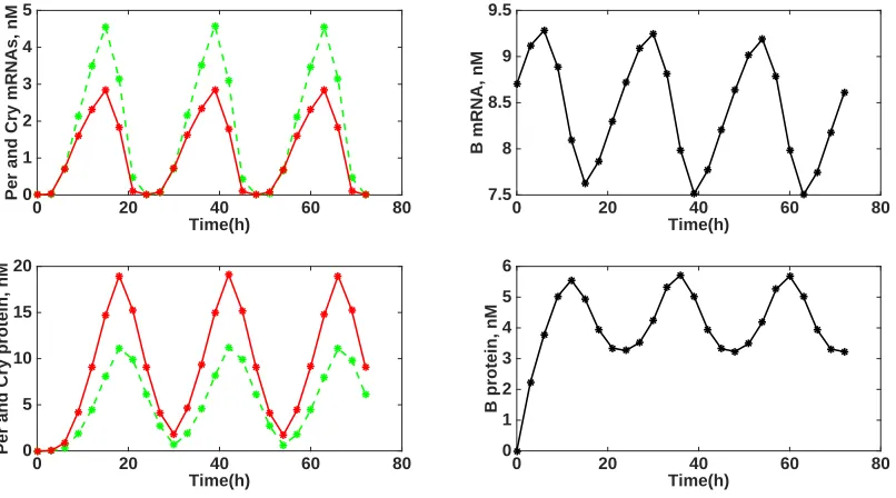
We sought to determine whether optimizing system perturbations could improve confidence in parameters es-timated for a system with a dynamic (i.e., periodic) equilibrium, using the circadian rhythms model as a test example. Below, we analyzed forward solutions and uncertainty quantification plots resulting from the parameter subset selection algorithm using a naive or optimal experimental design for several different choices of the final experiment time (tf), the observation frequency, and the number of possible perturbations (H). The sensitivity matrix is evaluated at the discrete time points determined by the observation frequency. The forward solutions are presented in a similar style to those in Figure 2 of [9], where the total amount ofPer,Cry, andBmal1 mRNAs and PER, CRY, and BMAL1 proteins are presented. The parameter subset selection graphs are the plots of the normalized standard errors for each parameter in the set P. It is important to note that the subset selection algorithm does not re-estimate parameters when minimizing the selection score; the Fisher Information Matrix is calculated only once, from which respective rows and columns are removed to calculate standard errors. We note that re-estimation following the application of the subset selection algorithm was tested in [2] and proved to make only negligible differences in the results. We define a threshold at which parameter uncertainty can be taken as reasonable by setting an upper bound on the normalized standard error for each parameter in a given subset; this bound ensures that every 95% confidence interval is narrower than the parameter estimate itself. This value is represented by the horizontal (red) line in the subset selection graphs with the value ₁_.1₉₆ = 0.5102, as presented in [2].

(11)

Time(h)

0 20 40 60 80

Per and Cry mRNAs, nM 0

1 2 3 4 5

Time(h)

0 20 40 60 80

B mRNA, nM

7.5 8 8.5 9 9.5

Time(h)

0 20 40 60 80

Per and Cry protein, nM 0

5 10 15 20

Time(h)

0 20 40 60 80

B protein, nM

0 1 2 3 4 5 6

(12)

5.1 Optimal Experimental Design:

t

_f

_{= 72}

_{hrs, observation frequency = 3 hrs,}

H

_{= 3}

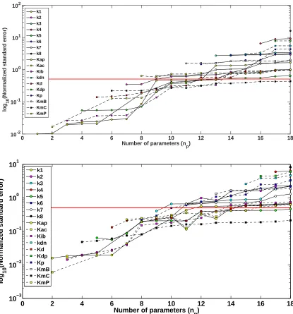
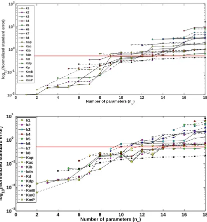
We first investigated whether introducing RNAi perturbations, calculating using our optimal experimental design algorithm (Equations (29) - (30)), could have an affect on reducing parameter uncertainty. We implemented our optimization algorithm using an experimental time of 72 hours, an observation frequency of 3 hours, and 3 time intervals for possible RNAi activation/deactivation (H = 3). Using 3 possible perturbation intervals, we found that the optimal time mesh s and perturbation vector b corresponding to the function u(t;b, s) were equal to

{0,16.8410,47.0857,72}and{0,1,0}, respectively. Figure 2 (top) displays the naive experimental design results with comparison to the optimized experimental design results (bottom) with regard to parameter uncertainty as calculated using the subset selection algorithm. As stated previously, all of the parameter subset selection graphs were plotted on a logarithmic scale due to the substantial difference of the normalized standard errors (NSEs). Specifically, the NSEs for each parameter were calculated using a parameter subset selection algorithm and are plotted log10 scale fornp= 1, ...,18 chosen parameters.

We found that an optimized experimental design produced improvement in parameter uncertainty. The sum of the NSEs atnp= 18 for the naive and optimal experimental design were 63.9709 and 43.2897, respectively. We also observed an overall decrease in the NSEs for each of the parameters chosen by the subset selection algorithm at all values of np = 1, . . . ,18. For example, the NSE for KmC estimated at np = 18 is less for the optimal experimental design (0.2144) than for the naive experimental design (0.4363), and similar results were found for the other parameters in the model at all values ofnp. Moreover, two parameters were below the 95% confidence interval threshold at np = 18 vs. only 1 parameter for the naive experimental design (Figure 2). Specifically, only the NSE forKmC completely falls below the threshold set at.5102 for both naive and optimal experimental designs. However, the NSE for k5 also falls below the threshold for the naive and experimental designs for all

(13)

Number of parameters (n

p)

0 2 4 6 8 10 12 14 16 18

log

10

(Normalized standard error)

10-2 10-1 100 101 102

k1 k2 k3 k4 k5 k6 k7 k8 Kap Kac Kib kdn Kd Kdp Kp KmB KmC KmP

0 2 4 6 8 10 12 14 16 18

10−3 10−2 10−1 100 101

p)

log

10

(14)

5.2 Optimal Experimental Design:

t

_f

_{= 72}

_{hrs, observation frequency = 3 hrs,}

H

_{= 5}

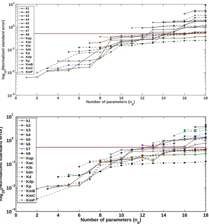
We investigated whether increasing the number of possible time intervals for the RNAi perturbation could have a greater affect on reducing parameter uncertainty. We implemented our optimization algorithm using an ex-perimental time of 72 hours, an observation frequency of 3 hours, and 5 time intervals for possible RNAi acti-vation/deactivation (H = 5). Using 5 possible perturbation intervals, we found that the optimal time mesh s

and corresponding perturbation vectorbdefiningu(t;b, s) were equal to{0,16.7561,38.7894,44.5964,70.0176,72}

and{0,1,1,0,0}, respectively. Figure 3 (Top) displays the naive experimental design results with comparison to the optimized experimental design results (Bottom) with regard to parameter uncertainty as calculated using the subset selection algorithm.

We found that, although an optimal experimental design with H = 5 did have an impact on parameter uncertainty as compared to the naive experimental design, it was not very different from the case with H = 3 (Figure 3). For example, the sum of the NSEs for H = 3 and H = 5 for np = 18 were 43.2897 and 43.1881, respectively. Likewise, the maximum number of parameters that lay below the uncertainty threshold for an optimized experimental design was the same forH = 3 andH = 5, i.e.,np= 10.

(15)

p)

0 2 4 6 8 10 12 14 16 18

log

10

10-2 10-1 100 101 102

0 2 4 6 8 10 12 14 16 18

10−3 10−2 10−1 100 101

p)

log

10

(16)

Time(h)

0 20 40 60 80

1 2 3 4 5 Time(h)

0 20 40 60 80

B mRNA, nM

7.5 8 8.5 9 9.5 Time(h)

0 20 40 60 80

5 10 15 20

Time(h)

0 20 40 60 80

B protein, nM

0 1 2 3 4 5 6

0 20 40 60 80

0 2 4 6

Time(h)

Per and Cry mRNAs, nM 0 20 40 60 80

6 8 10

Time(h)

B mRNA, nM

0 20 40 60 80

0 10 20 30

Time(h)

Per and Cry protein, nM 0 20 40 60 80

0 2 4 6

Time(h)

B protein, nM

0 20 40 60 80

0 2 4 6

Time(h)

Per and Cry mRNAs, nM 0 20 40 60 80

6 8 10

Time(h)

B mRNA, nM

0 20 40 60 80

0 10 20 30

Time(h)

Per and Cry protein, nM 0 20 40 60 80

0 2 4 6

Time(h)

B protein, nM

Figure 4: Forward solutions of the circadian model for the naive and optimized experimental designs for thePer,

(17)

5.3 Optimal Experimental Design:

t

_f

_{= 72}

_{hrs, observation frequency = 1 hrs,}

H

_{= 3}

We investigated whether increasing the observation frequency from every 3 hours to every hour could have a greater affect on reducing parameter uncertainty when using our optimal design algorithm withH = 3. Using 3 possible perturbation intervals with a one hour observation frequency, we found that the optimal time meshsand corresponding perturbation vector bdefiningu(t;b, s) were equal to{0,15.6869,44.0767,72}andu(t) ={0,1,0}, respectively. Figure 5 (Top) displays the naive experimental design results with comparison to the optimized experimental design results (Bottom) with regard to parameter uncertainty as calculated using the subset selection algorithm.

Our results indicate that increasing the observation frequency when utilizing our optimal design algorithm may have a significant affect on lowering parameter uncertainty. In the case ofH = 3, the sum of the NSEs for

np= 18 parameters was lowered from 43.28 to 25.41 by increasing the observation frequency from 3 per hour to 1 per hour, respectively. The maximum number of parameters that lay below the uncertainty threshold for an optimized experimental design with 3 and 1 hour observation frequencies wasnp= 10 andnp = 12, respectively. There are 10 parameters below the uncertainty threshold atnp= 18 when using an optimized experimental design with 1 hour observation frequency and H = 3 (Figure 5 (Bottom)). In contrast, there are only 2 parameters that lie below the uncertainty threshold at np = 18 when using an optimized experimental design with 3 hour observation frequency andH = 3 (Figure 2 (Bottom)).

We note that increasing the observation frequency when using a naive experimental design could have a similar affect on parameter uncertainty as using an optimal experimental design. For example, we found that increasing the observation frequency to every hour when using a naive experimental design resulted in parameter uncertainty levels similar to results found when using an optimal experimental design with a 3 hour observation frequency andH = 3. For example, there are two parameters that lie below the uncertainty threshold atnp= 18 for both of these cases (compare Figure 5 (Top) and Figure 2 (Bottom)).

(18)

p)

0 2 4 6 8 10 12 14 16 18

log

10

10-3 10-2 10-1 100 101

0 2 4 6 8 10 12 14 16 18

10−3 10−2 10−1 100 101

p)

log

10

(19)

5.4 Optimal Experimental Design:

t

_f

_{= 320}

_{hrs, observation frequency = 3 hrs,}

H

_{= 3}

We investigated whether increasing the total experiment time from tf = 72 hours to tf = 320 hours could have an affect on reducing parameter uncertainty when using our optimal design algorithm with H = 3. Using 3 possible perturbation intervals with a 3 hour observation frequency, we found that the optimal time mesh s

and corresponding perturbation vector b defining u(t;b, s) were equal to {0.0005,108.7691,210.8853,313.3115}

and{0,1,0}, respectively. Figure 6 (Top) displays the naive experimental design results with comparison to the optimized experimental design results (Bottom) with regard to parameter uncertainty as calculated using the subset selection algorithm.

Our results indicate that increasing the total experiment time when utilizing our optimal design algorithm may have a significant affect on lowering parameter uncertainty. For example, in the case of H = 3, the sum of the NSEs fornp= 18 parameters was lowered from 43.28 to 11.3029 by increasingtf from 72 to 320, respectively (compare Figure 2 (Bottom) to Figure 6 (Bottom)). The maximum number of parameters that lay below the uncertainty threshold for an optimized experimental design for tf = 72 and tf = 320 hours were np = 10 and

np= 14, respectively. Likewise, the number of parameters that were below the uncertainty threshold atnp= 18 were 2 and 11 for the case whentf = 72 andtf = 320, respectively.

(20)

p)

0 2 4 6 8 10 12 14 16 18

log

10

10-3 10-2 10-1 100 101

0 2 4 6 8 10 12 14 16 18

10−3 10−2 10−1 100 101

p)

log

10

(21)

Time(h)

0 100 200 300 400

1 2 3 4 5

Time(h)

0 100 200 300 400

B mRNA, nM

7 7.5 8 8.5 9 9.5

Time(h)

0 100 200 300 400

5 10 15 20

Time(h)

0 100 200 300 400

B protein, nM

0 1 2 3 4 5 6

0 100 200 300 400 0

2 4 6

Time(h)

Per and Cry mRNAs, nM 0 100 200 300 400

6 8 10

Time(h)

B mRNA, nM

0 100 200 300 400 0

20 40 60

Time(h)

Per and Cry protein, nM 0 100 200 300 400

0 2 4 6

Time(h)

B protein, nM

Figure 7: Forward solutions of the circadian model for the naive and optimized experimental designs for thePer,

(22)

6 Discussion

Overall, our results suggest that experimental input manipulation that produces non-equilibrium system dynamics for oscillatory systems yields more informative data sets for parameter estimation than that obtained when using an unaltered or undisturbed system. In particular we obtain more statistical certainty in parameters for the model in the form of lower normalized standard errors. Optimization of the input manipulation with a piecewise constant functional form, i.e., via our iterative algorithm (Equations (29) and (30)), can successfully reduce standard errors in parameter estimates for the circadian system, and possibly among other models with dynamic equilibria. As shown unanimously in the graphs presented in the Results section, creating a perturbation in the dynamic circadian system at least results in lower normalized standard errors and often increases the number of parameters below the designated threshold. Increasing the observation frequency while calculating optimal system perturbations further reduces the normalized standard errors, as seen in Figure 5.

Interestingly, when the duration of the experiment was increased, the normalized standard errors decreased without the perturbation and even more so with the system disturbance. This was evidenced by Figure 6. The result matches intuition since the observation frequency of 3 hours is not related to the periodicity of the system’s oscillations; therefore, when the model is simulated for 320 hours, there is not yet any information repetition or selection of points with the same values at different times. The opposite of this would be selecting the maximum of each period at different times. The data would essentially be observed as constant, and the Fisher Information Matrix would not be invertible. Since the sensitivities are calculated at time points not dependent on the periodicity of the model oscillations, running the model for a longer period of time “discovers” more about the solution, thereby producing a Fisher Information Matrix without any similar columns or rows. As seen in Figure 6, perturbing the system away from this equilibrium only exacerbates this effect.

Future investigations will attempt to investigate possible parameter correlations by bootstrapping and calcu-lating standard errors through asymptotic techniques in the context of information theory. Provided raw data, another future investigation could consolidate the conclusion of this paper with inverse problem techniques and extrapolate these findings to the creation of optimal experimental designs.

7 Acknowledgements

This research was supported in part by the Air Force Office of Scientific Research under grant number AFOSR FA9550-12-1-0188, in part by the National Science Foundation by Undergraduate Biomathematics grant number DBI-1129214 and in part by the National Science Foundation under grant number DMS-0946431.

References

[1] K. Adoteye, H. T. Banks, K. B. Flores, Optimal design of non-equilibrium experiments for genetic net-work interrogation. CRSC-TR14-12, Center for Research in Scientific Computation, North Carolina State University, September, 2014;Applied Math Letters,40(2015), 84–89.

[2] H.T. Banks, Robert Baraldi, Karissa Cross, Kevin Flores, Chistina McChesney, Laura Poag, and Emma Thorpe, Uncertainty quantification in modeling HIV viral mechanics. CRSC-TR13-16, Center for Research in Scientific Computation, North Carolina State University, December, 2013;Mathematical Biosciences and

Engineering, to appear.

[3] H. T. Banks, A. Cintron-Arias, and F. Kappel,Parameter selection methods in inverse problem formulation,

inMathematical Modeling and Validation in Physiology, ser. Lecture Notes in Mathematics (eds. J. J. Batzel,

M. Bachar, and F. Kappel), Springer Berlin Heidelberg (2013), 43–73.

[4] H. T. Banks, K. B. Flores, K. Link, L. Poag, T. Huffman, and J. Nardini, A mathematical model of RNA3 recruitment in the Brome Mosaic Virus replication cycle,International Journal of Pure and Applied

(23)

[5] H. T. Banks, K. Holm, and F. Kappel, Comparison of optimal design methods in inverse problems,Inverse

Problems,27(2011) 075002.

[6] H. T. Banks, S. Hu, and W. C. Thompson,Modeling and Inverse Problems in the Presence of Uncertainty, CRC Press, Boca Raton (2014).

[7] H.T. Banks and H.T. Tran,Mathematical and Experimental Modeling of Physical and Biological Processes, CRC Press, Boca Raton London New York, 2009.

[8] A. Cintron-Arias, H. T. Banks, A. Capaldi and A. L. Lloyd, A sensitivity matrix based methodology for in-verse problem formulation, CRSC Tech. Rep. CRSC-TR09-09, April, 2009;J. Inverse and Ill-posed Problems,

17(2009), 545–564.

[9] Jean-Christophe Leloup and Albert Goldbeter, Modeling the mammalian circadian clock: Sensitivity analysis and multiplicity of oscillatory mechanisms,Journal of Theoretical Biology,230(2004), 541-562.

[10] Joaquim R. R. A. Martins, Ilan M. Kroo, and Juan J. Alonso, An automated method for sensitivity anal-ysis using complex variables, Proc. 38th Aerospace Sciences Meeting, paper AIAA-2000-0689, Amer. Inst. Aeronautics and Astronautics (2000), pp. 1–12.