Multidomain Medium Frequency Transformer Optimization Using High Fidelity Modelling.

(1)

ABSTRACT

BOOTH, KRISTEN ELIZABETH. Multidomain Medium Frequency Transformer Optimization Using High Fidelity Modelling. (Under the direction of Srdjan Lukic.)

Power electronic converters are the standard of power conversion. They enable

renew-able energy integration to the power grid as well as transfer AC grid power to DC required by

consumer devices, such as electric vehicles. These converters require multidomain design

to achieve high power density and efficiency.

Many of these converters require galvanic isolation in terms of a transformer. At lower

frequencies, these magnetic components, and any necessary resonant capacitors, can

be large. This reduced power density is a major disadvantage to many power electronic

converter applications, such as naval ship power systems. However, improvements in

semiconductors have enabled these converters to reach higher frequencies to reduce the

size of the reactive components, including the transformer. As the power density increases,

thermal limits become an inherent constraint of the design.

This work proposes an improved method of medium frequency transformer

optimiza-tion. By using previously documented analytical models and incorporating high fidelity

models into the optimization routine, a highly accurate and computationally efficient

algo-rithm is obtained. Furthermore, a robust optimization procedure is introduced to handle

parameter tolerances of the medium frequency transformer. The analysis shows that the key

variation in transformer feasibility are the thermal constraints. If these are not accurately

modelled, there is a high likelihood of an infeasible experimental setup. Adjustments can

be made to account for deviations that may occur to create a more conservative design.

This enables a feasible, true optimal design point that will require no adjustments in the

(2)

(3)

Multidomain Medium Frequency Transformer Optimization Using High Fidelity Modelling

by

Kristen Elizabeth Booth

A dissertation submitted to the Graduate Faculty of North Carolina State University

in partial fulfillment of the requirements for the Degree of

Doctor of Philosophy

Electrical Engineering

Raleigh, North Carolina

2019

APPROVED BY:

Iqbal Husain Wensong Yu

Scott Ferguson Srdjan Lukic

(4)

DEDICATION

(5)

BIOGRAPHY

Kristen Booth has taken a Postdoctoral Researcher position at The Ohio State University

in the Center for High Performance Power Electronics (CHPPE) after defending her Ph.D.

As an NSF Graduate Research Fellow, Kristen completed her Ph.D. degree from North

Carolina State University in 2019. She graduated from NCSU with a M.S. in Electrical

Engineering in 2017 and received the B.S.E. in Engineering Physics in 2015 from Murray State

University. Kristen’s research interests include resiliency and reliability of power electronics

converters, optimization of medium frequency transformers, and power electronics for

(6)

ACKNOWLEDGEMENTS

I would like to thank my advisor, Dr. Lukic, for the freedom to pursue my research interests.

I would also like to express my gratitude to everyone at the FREEDM Systems Center. The

friendships made along the way will always be remembered fondly. To Ken, Hulgize, Teri,

Roy, Pam, Karen, and Rebecca, your advice and laughter are what made FREEDM feel like

home. I’d like to give a special shout out to Rishabh and Erick for putting up with me as

cubicle mates. Our discussions made our work better. To Mehnaz and Likhita, thank you

for being you. I want to mention a few more, but by no means is this an exhaustive list:

Siddharth, Landon, Radha, David, Michelle, Awal, Megan, and Ali. We will forever be apart

of the FREEDM family.

By no means did my journey begin at FREEDM. I greatly appreciate the help of the

McNair Scholars program, including Leslie, and the resulting relationship with my first

research advisor, Dr. Leedy, at Murray State University. There aren’t enough words to express

how important you both are to me. I’d also like to acknowledge Stephanie, Verena, and Will

Leedy for their support and visits through the years.

For all the support through the years, thank you to my families. Mom and Dad, thank

you for your constant and irrevocable belief in me. Blake, Katie, Anna Grace, Amber, and

the Todd, love you long time. Mike, Tammy, Mikey, Marsha, Micah, Katy, and Adam, thank

you for your love and welcoming me into your family. To my grandparents, I know you’re

cheering me on from a better place. I also tip my hat to all the extended family, the Garcias,

the Runges, the Booths, and the Tarltons. Cheers to my lake family, the Hines, the Stewarts,

the Alexanders, and the Meltons. I also cherish my lifelong friends, Betty Kay, Aubrey,

Scarlett, and Jin. While we might have physical distance between us, our friendships will

(7)

To Ronnie Booth, what words are there left to say? We’ve had our share of ups and downs,

and you’ve been there to support me through it all. Thank you for riding this roller coaster

of life with me, and I can’t wait to see where we go together. I love you whole bunches.

Finally, thank you to the NSF Graduate Research Fellowship. This material is based upon

(8)

LIST OF TABLES

Table 2.1 Leakage Inductance Comparison . . . 32

Table 3.1 Core Losses at 25◦_{C . . . .} ₅₃

Table 3.2 Core Losses at Steady State Temperatures . . . 53

Table 3.3 Core Loss Percent Error Between Low and High Fidelity Models . . . . 54

Table 4.1 Transformer Design Specifications . . . 68

Table 4.2 Optimized Transformer Designs . . . 69

Table 4.3 Transformer Estimated Temperatures in Degrees Celsius . . . 70

Table 4.4 Transformer Design Specifications and Variables . . . 72

Table 4.5 Comparison of Optimization Model and Experimental Results . . . 81

Table 5.1 Parameter Tolerances . . . 86

Table 5.2 Relation ofk to Constraint Feasibility . . . 90

Table 5.3 Constraint Variance by Individual Parameter . . . 92

Table 5.4 Constraint Variance . . . 92

Table 5.5 Objective Variance by Individual Parameter . . . 93

Table 5.6 Objective Variance . . . 93

Table 6.1 XFC MFT Design Specifications . . . 101

Table 6.2 XFC MFT Analytical Losses . . . 107

(11)

LIST OF FIGURES

Figure 1.1 Design method comparison where a conventional design method is

on the left and optimization approach is on the right[2]. . . 2

Figure 1.2 GA algorithm flow chart. . . 7

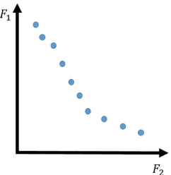
Figure 1.3 A Pareto front example. . . 9

Figure 1.4 Ranking designs in multi-objective optimization. . . 9

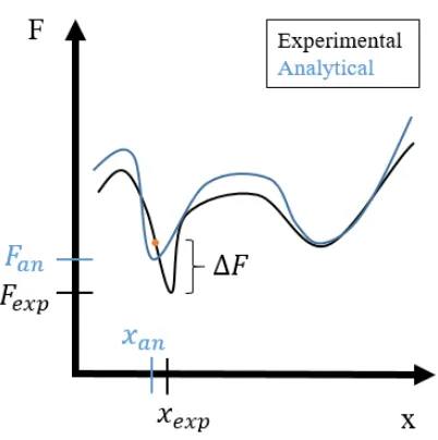
Figure 1.5 Generic model and experimental responses. . . 11

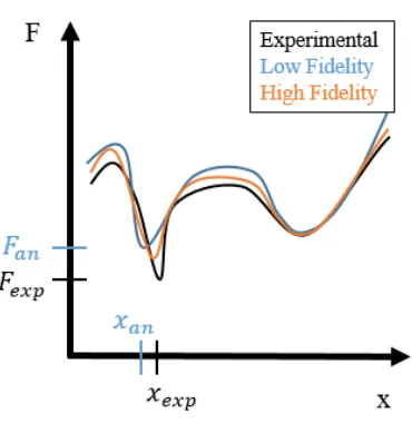
Figure 1.6 Responses of generic low and high fidelity models and experiment. . 13

Figure 2.1 Equivalent nonideal transformer circuit. . . 16

Figure 2.2 Skin effect in a winding at various frequencies: (a) surface distribution and (b) cross-sectional distributionJz(x)[94]. . . 19

Figure 2.3 Proximity effect on windings due to an external magnetic field: (a)surface distribution and (b) cross-sectional distributionJz(x)[94]. . . 20

Figure 2.4 Transition to foil windings from round conductors. . . 21

Figure 2.5 Core-type transformer vertical cross section. . . 26

Figure 2.6 Core-type transformer horizontal cross section. . . 27

Figure 2.7 MEC of core-type transformer. . . 27

Figure 2.8 Core-type transformer leakage paths. . . 28

Figure 2.9 Core-type (a) experimental transformer and (b) FEA model. . . 32

Figure 2.10 Domain wall movement: (a) without applied field and (b) with ap-plied field[87]. . . 33

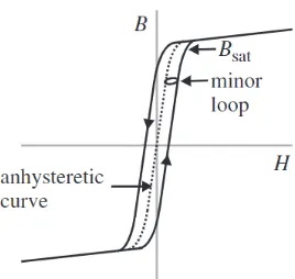
Figure 2.11 A generic B-H curve. . . 34

Figure 2.12 Comparison of i2_{GSE and iGSE}_[₇₀_]_{. . . .} ₃₈

Figure 2.13 Conversion comparison of square waveform to sinusoidal excitation. 39 Figure 2.14 Experimental core loss measurement circuit. . . 40

Figure 2.15 Percent error caused by sampling uncertainty in phase angle versus phase angle for differentN [97]. . . 41

Figure 2.16 Output of FEA for core losses. . . 42

Figure 2.17 An example of nonuniform flux density in a UU-core. . . 43

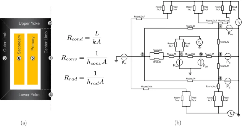
Figure 2.18 (a) Two-dimensional MFT structure with nodal temperature loca-tions. (b) Thermal resistive network for MFT design. . . 47

Figure 3.1 Analytical surface and FEA simulations using a constant 4-core model. 55 Figure 3.2 Proposed optimization algorithm for MFT. . . 65

Figure 4.1 Three-level LLC resonant converter with MFT. . . 68

Figure 4.2 FEA model of MFT. . . 71

(12)

Figure 4.4 Objective space of MFT optimization using Brute Force (circles), the Pareto front (squares), and experimental results of SOA (star) and

ASM (hexagram). . . 73

Figure 4.5 Experimental setup for full load test. . . 74

Figure 4.6 Core loss measurement method. . . 75

Figure 4.7 SOA full load experimental results. . . 76

Figure 4.8 Thermal FEA model results of SOA design and predicted nodal tem-peratures. . . 77

Figure 4.9 ASM full load experimental results. . . 79

Figure 4.10 Physical transformer for the ASM design with thermocouples. . . 79

Figure 4.11 Thermal FEA model results of ASM design and predicted nodal tem-peratures. . . 80

Figure 5.1 Sensitivity analysis of MFT. . . 87

Figure 5.2 Normal distribution of potential designs versus (a) efficiency and (b) power loss. The shaded area depicts 97.725% of potential designs due to tolerances. The red star is the SOA result, and the ASM result is shown as pink hexagram. . . 94

Figure 5.3 Normal distribution of potential designs versus (a) power density and (b) volume. The shaded area depicts 97.725% of potential designs due to tolerances. The red star is the SOA result, and the ASM result is shown as pink hexagram. . . 95

Figure 5.4 Optimization outcome with the potential design region highlighted in yellow. . . 95

Figure 5.5 Results of robust optimization of MFT design. . . 96

Figure 6.1 Optimization outcome with the potential design region highlighted in yellow. . . 99

Figure 6.2 Single-phase of the XFC modular layout. . . 100

Figure 6.3 Modulation scheme of the NPC DAB which contains the MFT. . . 100

Figure 6.4 Test configuration for BIL[99]. . . 102

Figure 6.5 (a) Passed impulse test. (b) Failed impulse test. . . 103

Figure 6.6 Applied voltage and PD test configuration[99]. . . 103

Figure 6.7 One half of the MFT with the bobbin structure. (a) Isometric view. (b) Front view. . . 106

(13)

CHAPTER

1

Introduction

1.1 Medium Frequency Transformers

The future of the power grid will be shaped by the evolving topologies in power electronic

converters. As distributed energy resources, such as residential and commercial

photo-voltaic arrays or wind turbines, are tied into the power grid, these converters are required

to stabilize grid-tied voltages and maintain grid synchronization. Solid State Transformers

(SSTs), an application of these converters, improve the reliability of the grid and voltage

regulation while also enabling reactive power compensation in smart grid concepts[42, 79,

100].

A key component of power electronic converters is the Medium Frequency Transformer

(14)

the separated electrical circuits. Designing MFTs is an incredibly difficult task due to the

incorporation of resonant components for resonant converters. This reduces the overall

size of the converter system. Due to the thermal and electrical requirements of MFTs,

multidomain modelling is invaluable to the design process.

As with all engineering challenges, the design process calls for an iterative procedure.

This includes design, test, and repeat until a desired response or criteria is met. Fortunately,

as processing power of computers has increased and more design programs have become

available, this methodology has been replaced by optimization techniques to reduce the

time and effort to an optimal design. These minute, but important, differences are described

in Fig. 1.1. Many of the steps are similar; however, lack of a fitness measurement of the

design and early termination of conventional design methods are the major disadvantages.

(15)

1.2 Optimization Algorithms

Before delving into optimization, some basic terms must first be described. Design

vari-ables are the inputs to the optimization algorithm and are given by the vector,x. They are

the “unknowns" that can be modified and may be continuous or discrete. In transformer

optimization, a few design variable examples are core area, core material, winding gauge,

and winding turns.

The function of design variables is the objective function,F(x). Optimization calls for a maximization or minimization of the objective function. Formalities of optimization

algorithms prefer minimizing the objective function; therefore, this will be the case in

this work. Objective functions may be unimodel, multimodal, or increase or decrease

monotonically. Common objective functions for transformer optimization are efficiency

and power density.

Constraints are limitations on the design and are a function of the design variables.

They may be in the form of side bounds,xL B_i ≤xi≤xU B_i ; inequalities,g(x)≤0; or equalities,

(16)

1.2.1 Problem Formulation

With these definition in mind, a formalized problem statement can be written. In general,

MinimizeF(x) Subject to:

gj(x)≤0 j =1 . . .m

hk(x) =0 k=1 . . .l xL B

i ≤xi≤x U B

i i =1 . . .n

(1.1)

where the side bounds are turned into two inequality constraints,

xL B_i ₋x_i_≤0 (1.2)

and

xi−xU Bi ≤0. (1.3)

When defining the optimization problem, it is imperative that the design variables,

objective function, and constraints are properly characterized. Poor choices may result in a

sub-optimized design or divergence. For some optimization algorithms to work properly,

the objective function must be equally sensitive to all design variables; therefore, each

design variable must have equal weight. This is accomplished through normalization. In

the same manner, constraints must have equal weight when violated to avoid one affecting

the fitness to a greater extent. Consider normalizing the constraint,

(17)

by modifying it to

g : σ(x)

σa l l o w a b l e

−1_≤0 (1.5)

whereσ(x)is the constraint value calculated using a particular design set,x, andσ_{a l l o w a b l e} is a maximum allowable constraint value.

1.2.2 Overview of Optimization Techniques

Depending on the optimization problem, a plethora of optimization algorithms can be

found in the literature. The type of optimization problem that can be solved is

corre-lated to the shape of the objective function. For a single-variable optimization, there are

approximation-based approaches, such as 3-point quadratic with refinement, or region

elimination methods, including golden section[2]. These require a convex objective

func-tion in the defined search space.

Solvingnvariable optimization problems requires more complicated algorithms. Zero

order methods, such as grid-based search, global random searches, or Powell’s method,

are extremely useful when the objective function is discontinuous or design variables

are discrete[2, 66]. However, they are slow to converge and computationally inefficient.

Higher order methods use gradient knowledge to make move decisions . Unfortunately,

these methods, examples being Steepest Descent or Newton’s Method, can be trapped in a

local minima if the original guess is poor and the objective function is multimodal. Other

methods to solve these optimization problems are linear programming and sequential

unconstrained minimization techniques[2]. These can be affected by the accuracy of the

(18)

1.2.2.1 Evolutionary Techniques

The aforementioned methods are inadequate for the size, scale, and difficulty level of the

transformer optimization, especially when multi-objective optimization is desired. The

remaining method to solve this optimization problem is by using an evolutionary approach.

These approaches are extremely effective for highly nonlinear, discontinuous functions and

are readily scalable to multiple objectives. There are a few disadvantages of evolutionary

approaches. They require more objective function calls due to the population size and are

based on randomizations, such as mutations and crossovers. Due to the randomization of

heuristic approaches, each run of the optimization may lead to a different solution. This

leads to the biggest drawback: evolutionary algorithms do not have a proof of convergence.

There are three main evolutionary optimization algorithms: Simulated Annealing (SA),

Particle Swarm Optimization (PSO), and Genetic Algorithms (GAs)[2].

SA only has one design point per iteration, unlike PSO and GAs. It replicates the slow

cooling methods of critically heated materials, like steel. At high annealing temperatures,

the steel atoms can move freely. As it cools, the movement of the atoms are reduced. Based

on this setup, SA can make large steps at first and smaller steps as the "temperature" is

lowered. SA generates a random probability of taking a step that has a larger objective

function than the value at the current iteration. This enables SA to step out of local minima

which is an improvement over previously mentioned methods[52].

PSOs and GAs have a user-defined number of designs per iteration. PSOs work by having

a communicative population that explores a design space. Each design point, or particle,

has knowledge of the global best solution found and past points explored by the individual.

This information is used to adjust the particle’s position and velocity for the next iteration.

(19)

to PSO adjust for this by adding inertia terms to reduce velocity buildup[15, 32]. Discrete

design variables must be mapped to a continuous function prior to using the PSO algorithm

[55]. PSOs are simple to implement for a single objective, but multi-objective functions

increase the complexity by using multiple swarms[45].

GA concept is based on the evolution seen in nature. In the same way that "survival

of the fittest" exists, only the most fit designs remain in the population and reproduce.

Weaker genes are removed from population as generations improve. The flow of a GA is

depicted in Fig. 1.2. Once an optimization problem has been defined, an initial population

is created and assessed. Assessment can be performed through a variety of methods. A

basic assessment is the objective function value at that design point; however, this is not

the only means to assess and rank members of the population. A fitness function can be

described that is based on the objective function value for the design, the distance to other

designs, and/or penalty functions for violating constraints[44].

(20)

Once a fitness function has been described, parent designs are selected to generate

children designs through crossover. Mutations may occur in the children to introduce

diversity and variability into the population. Children are also assessed in the same manner

as parents. Finally, the population is updated through a process called selection. Selection

can occur through tournaments, truncation, or fitness proportion - "Roulette Wheel."

The population that makes it through the selection process is the next generation

of designs for the GA. Each generation is similar to an iteration of the aforementioned

methods. The GA terminates by a user-defined method. Common termination methods

include a finite number of generations, the most fit design lacking significant improvement,

or little improvement in the overall average of the population. GAs easily handle discrete

design variables, discontinuities in the objective function, and multi-objective optimization.

Therefore, a GA will be used for this work.

1.2.3 Multi-objective Optimization

Where single objective optimization has one optimal design, multi-objective optimization

provides an entire set of optimal points. This set is called the Pareto front and is due to the

trade-offs associated with compromising between objectives. An example of a Pareto front

is shown in Fig. 1.3. A design vector,x∗, is defined to be Pareto optimal if there does not exist another design vector,x, such thatfi(x)≤fi(x∗)for alli =1 . . .k and fj(x)<fj(x∗)for at least one index j. In other words,x∗_{is Pareto optimal if there is no}_x_{that exists that is} better in every objective function. All design vectors on the Pareto frontier are considered

non-dominated[2].

All other design vectors are dominated. Each front behind the Pareto front increases

(21)

Figure 1.3A Pareto front example.

from the population, the next front with the same requirements using the Pareto optimal

definition has a rank of 2. This is continued until all design vectors have a rank. An example

of ranking is given in Fig. 1.4.

Figure 1.4Ranking designs in multi-objective optimization.

A well-defined Pareto front has uniform spacing between design vectors covering a wide

range of the design space. This is where fitness assessment modification is important. Two

key fitness parameters for multi-objective optimization are the rank and relative distance

(22)

1.3 Motivation of Research

State of the art for transformer optimization is based onassuming that the analytical

models used are accurate enough to give the optimal design point (for a single objective

optimization) or Pareto front (for a multi-objective optimization). Sometimes, models are

not accurate enough. A common method of avoiding inaccurate modelling is by

character-izing some behavior experimentally and using a Look Up Table (LUT) of the data in the

final optimization algorithm.

Another known method of adjustment is by model tuning. Models can be “tuned" to

experimental data to make them align. This may occur by slight parameter changes. This

is very common in most research. A key way to spot tuned models would be to see highly

convergent analytical and experimental data. Used sparingly, tuning is an acceptable form

of model adjustment. In drastic cases, it is highly unethical.

If a model is not approximating the underlying physics well, the next logical step is

to improve the model. Consider the evolution of Steinmetz’s equation[86]. Steinmetz

originally proposed the equation based on sinusoidal excitation at low frequency for core

loss calculations. His equation is based on empirical relationships. It is not a physics-based

model, but a curve fitting of the data collected. All empirical equations have limitations;

for the Steinmetz Equation, it was limited to sinusoidal waveforms. Future work employed

the original equation,Pv =k Bβ, but improved it to include the frequency dependence,

Pv =k f αBβ. Further adjustments to the equation can be found in GSE, iGSE, and i2GSE as discussed in Section 2.3.2.2.

A multitude of publications, such as the ones previously mentioned, are based on the

idea of building a better, more complex model. Within transformer design, this can also be

(23)

AC resistances or leakage inductances. Some models introduce porosity factors for non-foil

windings; others discuss winding height versus window height. The essence of these papers

is model tuning, changing one parameter to fit the data better.

Figure 1.5Generic model and experimental responses.

These models are assumed to beaccurate enough. Choosing a design point based on a

model and using it in experiments is a common inference of the literature which enables

the design process. Assume the responses,F, of the experiment and model are given in Fig.

1.5 withx being the variable design parameter. The model closely resembles the responses

of the experiment. IfF is to be minimized, there will be two different answers - one from the

model,xa n, and one from the experiment,xe x p. Assume that the researcher does not have access to a full data set of experimental values. To minimize the function, the analytical

model will be used. However, the response for that design parameter once built, in this

(24)

line, shown by the orange point. The response is∆F away from the minimal response. Also,

it is not thetrueoptimal design point,xe x p. Therefore, the design is near the optimal point, but not exactly. This concept can be further motivated ifx is an array of varying design

parameters. Hence, a small "shift" inxcould drastically change the design point altogether.

The field has finally reached a quandary. Overly specific models can not be generalized

when finely tuned or has limiting assumptions. At some point, these models approach the

high fidelity models that are the foundation of Finite Element Analysis (FEA) programs.

The next logical step then is to move to high fidelity modelling. Instead of being used only

for design verification, high fidelity modelsshouldbe exploited, especially for optimization

routines.

A key drawback of high fidelity modelling is the computational effort. For a single

design verification, it is not uncommon to use. However, in an optimization routine, the

time consumption of using detailed models would be extensive. For example, GAs require

multiple generations of design populations. Considern designs in the population with

G generations.n is generally chosen to be the minimum of 10xd wherexdis the number of design variables or 100. The number of generations can be predefined or based on

population fitness from one generation to the next. That would require the high fidelity

model to be computedn×G times. Since the high fidelity model could take minutes, or

hours in some cases, this would be infeasible to run for such a population.

Assume the analytical model in Fig. 1.5 is a low fidelity model. It is easy and fast to

compute compared to a high fidelity model, such as FEA. The high fidelity model is added

in Fig. 1.6. Ideally, it should be nearly identical to the experimental responses. Realistically,

there is a limitation to the accuracy of the high fidelity model. However, as long as the

high fidelity model is more accurate than the low fidelity model, then the resulting optimal

(25)

Figure 1.6Responses of generic low and high fidelity models and experiment.

fidelity model alone has already been dismissed due to computational effort, a hybrid

method that uses the advantages of both the low and high fidelity models is preferred. This

enables a highly accurate response with low effort and fast computation time.

Lastly, this approach will not be as lab-dependent as other models in the literature.

This statement means that no experimental characterizations are required prior to using

the algorithm. The only experiments needed will be to verify the output responses. This

enables independent use for any researcher with no prior information needed that cannot

be obtained from data sheets.

1.4 Research Goals

Based on the motivation of this work. There are two main goals of this work. What is the

effect of modelling error and parameter tolerances on the final optimized MFT design? Can

(26)

1.5 Outline of Chapters

The rest of this work is presented as follows. Chapter 2 reviews the analytical, experimental,

and FEA methods to compute various transformer characteristics based on the physical

background provided. Limitations of measurements and calculations are discussed where

necessary. An overview of the state of the art in MFT optimization is described in Chapter 3

where gaps in the literature are discussed for motivation of the future work proposed in

(27)

CHAPTER

2

Multidomain Modelling of Medium Frequency Transformers

Using mutual magnetic coupling, transformers enable power transfer from one circuit to

another. An ideal transformer is completely lossless and has perfect coupling between the

windings. Therefore, the windings have zero resistance, and the core has infinite

perme-ability and no energy storage. In the physical world, however:

1. Core materials do not have infinite permeability;

2. Windings do not have perfect mutual coupling;

3. Windings do inherently have losses; and

4. Energy is stored and dissipated in the core.

The most perfectly realized winding configuration will still have some leakage flux which

(28)

temperature. Due to the physical structure of the core, some minimum energy is required

to magnetize the transformer. This energy will be partially stored and dissipated in the core.

A nonideal transformer is modelled in Fig. 2.1.

Figure 2.1Equivalent nonideal transformer circuit.

This chapter is written to correlate with the flow of the optimization routine. First, some

basic magnetic design background is described. This is followed by transformer parasitics.

The second half of this chapter deals with transformer losses and the thermal modelling.

2.1 Magnetic Design

Magnetic design for MFTs is usually built on the well-known models using area product.

There is some debate on the accuracy of the low frequency models in the medium frequency

applications[8]. However, these models are a good starting point for the MFT design process

as there is no proof that this method is inaccurate. Assuming that the designer knows some

basic information about the input and output(s) of the MFT (e.g. desired voltages, currents,

(29)

The optimization algorithm assumes knowledge of the input current,Ip r i; primary and secondary voltages,Vp r i andVs e c respectively; primary turns,Np r i; number of cores (size of core),Nc o r e; duty cycle,D; and a switching frequency,fs w. Using this information in the ideal transformer model, the turns ratio,a, the secondary turns,Ns e c, and the flux density,

B, calculations are shown in (2.1), (2.2), and (2.3) wherekf is a constant depending on the voltage waveform. It is equal to 4 for square waves and 4.44 for sine waves.

a =Vp r i Vs e c

(2.1)

Ns e c =

Np r i

a (2.2)

B= Vp r iD kffs wAcNp r i

(2.3)

Now that the basic information is available, the current density, J for each winding

must be calculated in order to choose the correct winding size,

Jy =

Iy

Aw,y

≤Jm a x,g a u g e, (2.4)

whereJm a x,g a u g e is the maximum current density for the equivalent gauge of the Litz wire andy can be either the primary or secondary winding.

The winding area is then

Aw,y =

NyAc u,y

kc u,y

(2.5)

(30)

The first check to eliminate infeasible designs is

kc u,c a l c =

Np r i(Aw,p r i) +Ns e c(Aw,s e c)

WA

≤kc u,c h o s e n (2.6)

whereWAis the window area.

The second check that can eliminate any infeasible designs is the area product,

AP =D[Vp r i(Aw,p r i) +Vs e c(Aw,s e c)] kf fs wB kc u

, (2.7)

where the following relationship must be true

AP≤WAAc o r eNc o r e (2.8)

and Ac o r e is the cross sectional area of the core. If a design is still feasible after these calculations, it will continue to the next section.

2.2 Winding Characteristics

2.2.1 Frequency Effects

Calculating copper resistances in MFTs is important to the thermal modelling of the

trans-former; however, the behavior of the current density and magnetic fields within the windings

are highly nonuniform at these frequencies. Skin effect is the behavior of current to flow

(31)

(a) (b)

Figure 2.2Skin effect in a winding at various frequencies: (a) surface distribution and (b) cross-sectional distributionJ_z(x)[94].

can be easily calculated to find the skin depth distanceδusing

δ=

v

t ρ

πµf =

v

t 2

ωµσ (2.9)

whereρ is the resistivity of the material,µis the permeability of the material, f is the

frequency of the waveform,ωis the angular frequency of the waveform, andσrepresents

the conductivity of the material. This equation easily calculates the distance the current

density penetrates until it reaches a factor of 37% of the original value as seen in Fig. 2.2

[78].

Due to the current flowing in the individual conductors, each conductor produces a

magnetic field that radiates into other nearby conductors, inducing unwanted voltages.

This natural response is called the proximity effect and forces an even more nonuniform

current density within affected conductors as seen in Fig. 2.3. The extent to which the

conductors are affected is based on the distance to other conductors and the time-varying

(32)

density; therefore, proximity effect cannot be avoided in designing MFTs due to the tight

packing of the windings.

(a) (b)

Figure 2.3Proximity effect on windings due to an external magnetic field: (a)surface distribution and (b) cross-sectional distributionJz(x)[94].

2.2.2 Winding Loss and Parasitic Calculations

There are several models to calculate AC resistance and leakage inductance. The most

widely used method for both is Dowell’s method. Many improvements on this method

have accumulated in the literature. Other lesser known models are also be discussed briefly

for their advantages and disadvantages. However, for the ease, simplicity, and accuracy of

Dowell’s method, it will be incorporated in the MFT optimization routine.

2.2.2.1 AC Resistance

Dowell’s method to calculate AC resistance can be used for a variety of winding

(33)

frequency-independent and -dependent calculations. The base assumptions of the method are that (i)

the winding layers completely occupy the window height of the core, (ii) the magnetic core

has infinite permeability as to only calculate the magnetic field in the transformer window,

and (iii) analysis is only in one dimension. The input current waveform information is also

needed for this method.

While foil conductors can be immediately imported to the model, round conductors

require some manipulation prior to using Dowell’s method to correlate to a foil winding.

This is done by creating a square conductor with the same cross-sectional area as the

original. The diameter of the conductor,dr, is converted by

de q =

sπ

4dr (2.10)

as depicted in Fig. 2.4.

Figure 2.4Transition to foil windings from round conductors.

The frequency-independent resistance calculation is merely the DC resistance of the

winding,

RD C =

mρNtlT

hwdw

(34)

whereRD C is the DC resistance per winding section,m is the number of whole foil layers in a winding portion,Nt is the number of turns per layer,lT is the mean turn length,hw is the winding height, anddw is the winding width. The summation of theseRD C of each winding portion is the total DC resistance of the winding. This is done for both the primary

and secondary windings separately.

The AC resistance is calculated using the AC resistance factor,Fr, as

RAC =FrRD C. (2.12)

In the case of nonsinusoidal current excitation, each harmonic,n, affects the skin depth,

δ0₌ δ

p

n, (2.13)

and the penetration ratio,∆

∆0₌p_n_∆₌p_ndw

δ . (2.14)

Finally, the AC resistance factor at each harmonic,Fr,n, can be defined as

Fr,n=∆0

ϕ0 1+ 2 3 m 2

−1ϕ₂0 (2.15)

where

ϕ0 1=

s i n h(2∆0₎₋_{s i n}₍₂_∆0₎

c o s h(2∆0)₋_{c o s}(₂∆0) (2.16)

and

ϕ0 2=

s i n h(∆0₎₋_{s i n}₍_∆0₎

c o s h(∆0)₋_{c o s}(∆0). (2.17)

(35)

between the windings. Therefore, the porosity factor,

η=hw

hc

=dw

p , (2.18)

is developed and introduces complexities in the skin depth and penetration ratios as

adjusted in (2.19) and (2.20) wherehc is the height of the core window[64].

δ00₌ δ0

p_η (2.19)

∆00₌p

η∆0 _(2.20)

These modifications flow through toϕ00

1 andϕ200by replacing∆0with∆00. Finally, the AC resistance factor is modified to

Fr,n=∆00

ϕ00 1+ 2 3 m 2

−1ϕ₂00. (2.21)

Therefore the total power loss for a current,Ir m s, is

Pc u,l o s s= ∞

X

n=1

Fr,nRD CI_{r m s}2 _,_n. (2.22)

Unlike Dowell’s method, Ferreira proposes a two-dimensional model to calculate AC

resistances of round conductors without converting them to foil-like conductors to improve

the accuracy at low winding porosities[39]. Unfortunately, it is based on a model describing

an isolated single conductor. As windings are condensed into a single area, proximity effects

are not included in the model, and this creates inaccuracies as described in the extensive

study found in[51]. The complexities of this method do not vastly improve the analytical

(36)

2.2.2.2 Leakage Inductance

Dowell’s method also extends to calculating leakage inductance using similar methods

applied in the AC resistance calculations[35]. Therefore, the modified Dowell’s method to

include the porosity factor is

Ll k=µ0N_{p r i}2

lT

hw

dw,p r imp r i

3 Fw,p r i +

dw,s e cms e c

3 Fw,s e c+cp s

+dw i,p r i

(mp r i−1)(2mp r i−1) 6mp r i

+dw i,s e c

(ms e c−1)(2ms e c−1) 6ms e c

(2.23)

where

Fw,y = 1 2m2

y∆

(4m2_y−1)ϕ₁₋2(m_y2−1)ϕ₂, (2.24)

lt is the mean turn length,my is the number of equivalent layers,cp sis the gap between the primary and secondary windings,dw,y is the equivalent winding width, anddw i,y is the width of the dielectric between layers.

2.2.2.3 Improvements to Dowell’s Method

For Litz wire, the porosity factor can be calculated as

η=Ns vde q

hw

(2.25)

due to the inconsistencies of Litz wire bundles that do not make a perfect matrix of windings

within the bundles[64]. This makes calculating the number of windings oriented

(37)

that the total winding cross-sectional profile is followed by the individual strands as

Kw=

hw

de q

. (2.26)

Thereby the horizontal and vertical number of windings can be calculated in (2.27) and

(2.28), respectively, whereNs is the number of strands in the Litz wire.

Ns h=

v tN_s

Kw

(2.27)

Ns v=

p

KwNs (2.28)

This avoids the need to calculate the porosity factor based on the harmonic number of the

current waveform.

Further correction, in[64], is made to the leakage inductance calculation by introducing

a correction, called the Rogowski factor, that adjusts the equivalent length of the magnetic

flux. The Rogowski factor can be calculated as

KR=1−

1₋e−πhw/(dw,p r i+dd+dw,s e c)

πhw/(dw,p r i+dd+dw,s e c)

(2.29)

and creates the improved height,

he q =

hw

KR

. (2.30)

Thishe q can replace thehw in (2.23) to gain a more accurate leakage inductance value when the windings do not stretch the entire core height. This improved method is used in

(38)

2.2.2.4 Magnetic Equivalent Circuit

Another method for calculating leakage inductance is via a Magnetic Equivalent Circuit

(MEC). While Dowell’s method is successful for shell-type transformers, MEC attempts to

handle core-type transformers[87]. In general, core-type transformers cause difficulty in

accurately calculating the leakage inductance since the leakage flux is inside the window of

the core as well as outside of the core. A core-type transformer with separated windings is

depicted in two planes in Fig. 2.5 and Fig. 2.6 with the relevant dimension definitions.

Figure 2.5Core-type transformer vertical cross section.

This setup produces the MEC shown in Fig. 2.7. The leakage inductance is defined as

Ll k,y =

N2

y

IR =IPN 2

Y (2.31)

(39)

Figure 2.6Core-type transformer horizontal cross section.

(40)

Figure 2.8Core-type transformer leakage paths.

Fig. 2.7 can be calculated by considering the leakage paths depicted in Fig. 2.8. It can be

seen that the paths vary based on the winding location, interior or exterior to the core. To

define whether the winding is interior exterior to the core, an angle,

αy =sin−1

2rc

ri,y +ro,y

, (2.32)

defines the point where the winding transitions from interior to exterior as shown in Fig. 2.6.

Then, the lengths of the interior and exterior portions of each coil are

li,y =lc,y +αy(ri,y+ro,y) (2.33)

and

(41)

into two parts,

IP_{p l} =IP_{p l i}+IP_{p l e}, (2.35) which are the interior and exterior leakage flux paths. The final derivations of these values

are given in

IPp l i=

µ0li,p r i

4k4

p i2+8kp i1kp i3 2+2k 2 p i1k

2 p i2−2k

3

p i1kp i2+4kp i41ln

1+2kp i2 kp i1

128w_w2_,_{p r i}d_w2_,_{p r i}

+ µ0li,p r i (hc+dw,p r i)

₁

2cc,p r i + 1 cp s

+(2ww,p r i+cc,p r i+cp s) cv,p r i

(2.36)

where

kp i1=|ww,p r i−dw,p r i| (2.37)

kp i2=min(ww,p r i,dw,p r i) (2.38) and

IPp l e =

µ0le,p r i

16k4 p e2+16

p

2kp e1kp e3 2+4k 2 p e1k

2 p e2−2

p

2k3

p e1kp e2+4k 4 p e1ln

1+2 p

2kp e2 kp e1

128w2

w,p r idw2,p r i

+ µ0le,p r iw

2 e p

ww,p r i(2we p) +

q

(2dw,p r i+2we p)(2we p3 ) (2.39)

where

kp e1=|dw,p r i−2ww,p r i|, (2.40)

kp e2= 1

p

(42)

and

we p=wc e c +0.5(hc−dw,p r i). (2.42) The secondary winding leakage is calculated in the same way due to the identical setup

by replacingp withs. Leakage inductance for each winding can then be calculated and

referred to the primary to reach the total leakage inductance.

2.2.3 Experimental Measurements for Leakage Inductance

Using an LCR meter, three measurements of the MFT can be made that will aid the leakage

inductance calculations: (i) the primary short-circuit inductance,Ls c

p r i, (ii) the primary open-circuit inductance,Lo c

p r i, and (iii) the secondary open-circuit inductance,L o c s e c.L

s c p r i is measured by shorting the secondary windings while the other two measurements are

made with the opposite winding being left open.

The inductive coupling coefficient,k, of the windings is found by rearranging

L_{p r i}s c =Lo c_{s e c}(1₋k2). (2.43)

The magnetizing inductance,Lm, referred to the primary can be defined as

Lm=Lo c_{p r i}k. (2.44)

Then, the primary leakage inductance, Ll k,p r i, and the secondary leakage inductance,

Ll k,s e c, are given in (2.45) and (2.46) wherea is the turns ratio.

(43)

Ll k,s e c =

Lm

a2 −L

o c

s e c (2.46)

By referring the leakage inductance to the primary, the total leakage inductance of the

transformer is

Ll k=Ll k,p r i+a2Ll k,s e c =Ll k,p r i+L0l k,s e c. (2.47)

2.2.4 Leakage Inductance Using FEA

Using the ANSYS Maxwell magnetostatic solution type, data fork, the self inductance of the

primary and secondary windings,Lpp andLss, respectively, and the mutual inductance,

M, can be obtained. The leakage inductance can be calculated via

Ll k,p r i =Lp p−a M, (2.48)

Ll k,s e c =Ls s−

M

a , and (2.49)

Ll k=Ll k,p r i+a2Ll k,s e c =Ll k,p r i+L0l k,s e c. (2.50)

2.2.5 Model Limitations

Dowell’s method and MEC are extremely accurate for the cases generally seen in MFTs –

tightly packed windings inside core windows – using one-dimensional models. However,

these models struggle to handle the leakage inductance calculation outside the core

win-dow found in the case of core-type transformers. This is due to the winding not being fully

encompassed by the core in the single plane prescribed in the models. Core-type

trans-formers, therefore, are not generally used in MFT design although core-type transformers

(44)

(a) (b)

Figure 2.9Core-type (a) experimental transformer and (b) FEA model.

Table 2.1Leakage Inductance Comparison

(mH) Experimental Analytical FEA

Ll k,p r i - 0.836 1.06

L0

l k,s e c - 0.586 0.283

Ll k 2.45 1.42 1.35

For example, a 60:10 UU core-type transformer was built for the electric vehicle fast

charger converter as shown in Fig. 2.9. Table 2.1 shows a comparison of the experimental,

analytical calculations, and FEA results of the leakage inductance.

2.3 Core Characteristics

Physical core characteristics cause losses to occur as energy is stored and transferred

through the magnetic material. This section discusses the causes of the core loss, and

several methods of calculation are described in varying detail based on popularity and

(45)

(a) (b)

Figure 2.10Domain wall movement: (a) without applied field and (b) with applied field[87].

2.3.1 Core Losses

Hysteresis and eddy currents are two sources of core loss. Hysteresis is a phenomenon

that occurs due to the moving magnetic domain walls as depicted in Fig. 2.10[87]. These

domains are the small portions of the material where adjacent atoms have aligned magnetic

moments. The net magnetic moment of the material is zero when there is no external

mag-netic field. When an external magmag-netic field is applied, these domain walls shift as domains

aligned with the field enlarge and all others reduce in size and magnitude. Saturated flux

density is the point at which all aligned domains occupy the entire material. Energy is

required to make these shifts and is a large portion of the total core losses. Hysteresis can

be seen in the generic B-H curve depicted in Fig. 2.11. The area inside the loop represents

work done on the material by an applied field and is dissipated in the form of heat[68].

Eddy currents affect the magnetic material due to the material also having good electrical

conductivity[38]. Therefore, the AC magnetic fields induce currents in the material to

oppose the flux as described by Lenz’s law. Excess eddy currents account for the differences

found between measured losses and the calculated hysteresis and eddy current losses. This

(46)

Figure 2.11A generic B-H curve.

localized near the domain walls[69]. A detailed discussion on magnetic domains is provided

in[98].

2.3.2 Core Loss Models

There are three common methods of core loss: loss separation, hysteresis, and empirical

methods. Loss separation handles each individual cause of core loss, as described in the

previous section, separately and sums all losses together:

Pl o s s =Ph y s t+Pe d d y+Pe x c e s s (2.51)

as first proposed by Bertotti[18]. Separating the losses is considered difficult and time

consuming as many material characterizations are required.

Hysteresis methods are physics-based and highly accurate; however, they also require

intensive material characterization. Empirical models are educated guesses based on

ex-perimental data. In essence, the data is curve-fit in relation to a few material-dependent

(47)

2.3.2.1 Hysteresis Methods

There are two affluent hysteresis-based models: the Preisach model [76] and the

Jiles-Atherton method[48]. Comparisons of these models with empirical methods for calculating

core losses prove that the characterizations needed are extremely time consuming, and

empirical methods are nearly as accurate with information provided by the manufacturer.

For these reasons, these models will not be discussed in detail and will not be used in this

work.

2.3.2.2 Empirical Methods

A multitude of empirical methods are described in the literature. These methods are based

on measurement observations. Many are based on the original Steinmetz equation[85, 86].

While Steinmetz did not include the frequency dependency, this power loss equation is

attributed to him:

Pc =K fs wα B

β

m. (2.52)

In (2.52),Pc is the core loss per unit volume,K,α, andβare Steinmetz coefficients, andBm is the peak flux density value of the AC waveform.αis a value between 1 and 2 depending

on the magnetic material, andβ is between 2 and 3. This method assumes a sinusoidal

waveform which is not valid in MF converters. A full review of Steinmetz equation-based

methods is given in[93].

Modified Steinmetz Equation

The first method to improve the Steinmetz equation for nonsinusoidal excitation is

introduced in[1]and relates the core loss to the derivative of flux density,dB/dt, by replacing

the frequency with an equivalent frequency as a function ofdB/dt. Reference[77], which

(48)

concise equation for core loss as compared to[1]. The literature suggests that MSE is more

inaccurate than other methods proposed[58]. MSE is defined as

Pc =

K f_{e q}(α−1)B_mβfr (2.53)

where

fe q = 2

∆B2π2

Z T 0 d B d t 2

d t, (2.54)

∆B=Bm a x −Bm i n, and fr=T1r is the remagnetization frequency. However, this method is not consistent with the original Steinmetz equation for sinusoidal waveforms[94].

General Steinmetz Equation with Improvements

General Steinmetz Equation (GSE) is based on the core loss being a function of the

instantaneous values of flux density and its rate of change as proposed in[56].

Pc(t) =Pd

d B(t) d t ,B(t)

(2.55)

Therefore,[58]proposes GSE,

Pc = 1 T Z T 0 k1

d B(t) d t

α

|B(t)|β−αd t; (2.56)

however,[91]shows that depending only on instantaneous values is a problem in practice

which results in inaccurate estimates.

Therefore, two separate research groups proposed a similar equation with a dependence

on instantaneous rate of change and the peak-to-peak amplitude of the flux density. They

are given credit for this model with two names, improved General Steinmetz Equation

(49)

reduced to the same expression:

Pc = 1 T Z T 0 ki

d B(t) d t

α

|∆B(t)|β−αd t (2.57)

where

ki=

K

(2π)α−1R2π

0 |cosθ|α2β−αdθ

. (2.58)

The key advantage to this method is the dependence only onK,α, andβ that is already

given by the manufacturer. iGSE is the most widely used core loss empirical method for

MFTs as it reduces to a simple equation for square wave excitation found in MF converters.

The latest improvement on the GSE is the improved-improved General Steinmetz

Equa-tion (i2_GSE)_[₇₁_]_{. This method aims to improve iGSE to account for relaxation in magnetic}

material. However, it hasn’t managed to become more popular than iGSE due to the need

for material parameters beyond the ones given by the manufacturer:

Pc = 1 T Z T 0 ki

d B(t_)

d t α

|∆B(t)|β−αd t+

n

X

l=1

Qr lPr l (2.59)

wherePr l is calculated for each voltage change as

Pr l = 1

Tkr

d d tB(t)

αr

(∆B)βr ₁₋_e− t₁

τ_, _(2.60)

Qr l =e−qr

d B_{d B}(₍t_t+)/d t

_)/d t

, (2.61)

andαr,βr,kr,τ, andqr are the new material parameters.t1is the length of time used to let the material reach thermal equilibrium used to findαr,βr, andkr in

∆E =kr

d d tB(t_)

αr

(50)

The material parameterτcan be found using

∆E

τ =

d E

d t , (2.63)

andqrmust be found by matching the model to the measured points of a duty cycle measure. These changes correct the mismatch at lower duty cycles, as shown in Fig. 2.12 and have

continuity with iGSE atD =0.5. While the data is well-modelled by the improvements described, it is lacking the simplicity usually preferred in analytical modelling. Therefore,

the iGSE method will be used in the optimization algorithms of this work.

Figure 2.12Comparison of i2_{GSE and iGSE}_[₇₀_]_.

Waveform Coefficient Steinmetz Equation (WcSE)

WcSE, in (2.64), works to replicate the flux density in a sinusoidal excitation by using

a conversion ratio to handle nonsinusoidal excitation. Shen derives conversion ratios for

several common excitation waveforms[80]. For example, a square waveform has a

(51)

but is known to be very inaccurate when a large zero voltage period is implemented in the

converter[93].

Pc = (F W C)K fαBmβ, (2.64)

Figure 2.13Conversion comparison of square waveform to sinusoidal excitation.

The total losses of the MFT have material dependencies that are related to the

corre-sponding temperature and peak flux density of the core. Therefore, the loss and thermal

calculations must be iteratively analyzed until there is relatively little change in the current

and previous loss calculations and nodal temperatures of the MFT.

2.3.3 Experimental Measurements of Core Loss

A wattmeter can be used to directly measure the electrical power of a system. However,

this technique breaks down as the system frequency and harmonic content increase. This

method is unsuitable for medium frequency magnetic measurements.

(52)

Figure 2.14Experimental core loss measurement circuit.

periodicv(t)andi(t), the generic power loss equations is

P = 1

T Z T

0

v(t)·i(t)d t. (2.65)

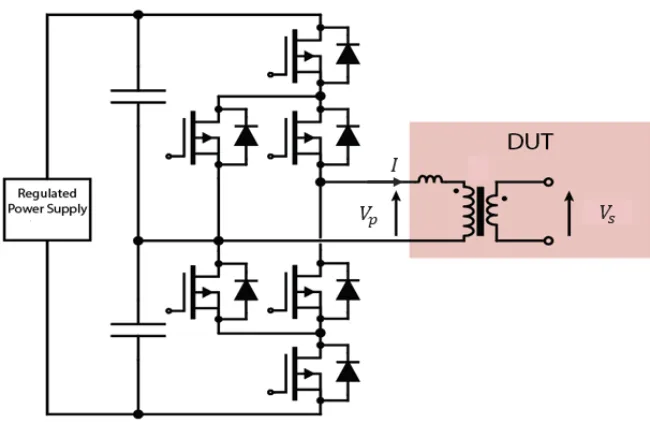
The experimental setup, shown in Fig. 2.14, is the most widely used core loss setup for its

ease in implementation throughout academia and industry although it is not considered

the most accurate[88, 97]. An excitation circuit creates the square voltage waveform across

the transformer primary terminals while the secondary terminals remain open-circuited.

When the open circuit voltage and primary current are measured, the resulting power loss

is the core loss. Since most oscilloscopes are digital with some sampling frequency,fs. For the sampled datav(ti)andi(ti), the average power can be approximated as

Pd= 1

N

N−1

X

n=0

(53)

whereN is the number of samples. These two equations assume that the primary and

sec-ondary winding turns are equivalent. Figure 2.15 shows the inaccuracy caused by sampling

uncertainty in phase angle versus percent error for various sampling rates over a cycle.

Since core loss measurements are based on a no-load setup[43, 88], the phase angle will

naturally be near 90◦_{. Calorimeters are a time-consuming method to improve transformer} loss measurements, but the winding losses and the core losses cannot be separated in this

method[61, 62, 96].

Figure 2.15Percent error caused by sampling uncertainty in phase angle versus phase angle for differentN [97].

2.3.4 Core Loss Using FEA

ANSYS can also be used to measure core loss by transiting to the transient solution type.

After collecting the required material characterizations from the data sheet for the design,

the instantaneous core losses are calculated and can be averaged for comparison with

(54)

Figure 2.16Output of FEA for core losses.

2.3.5 Model Limitations

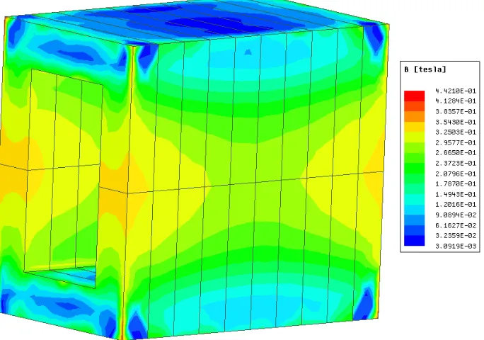
The common denominator that limits these analytical models for core loss is the assumption

of a uniform instantaneous flux density. It is well understood that flux density in a core

is highly nonuniform based on core structure and manufacturing process. For toroidal

cores, the flux density is largest near the center and is smaller near the outer edge. Any core

structures that have sharp corners, such as U-cores or E-cores, have little to no flux density

in the outer corners with a much larger proportion near the inner corners. An example of

this is given in Fig. 2.17 using FEA. Using high fidelity modelling, this assumption can be

removed to better model the physical phenomena occurring in the MFT.

2.4 Thermal Characteristics

After identifying the core and winding losses, the steady state temperatures of the core must

(55)

Figure 2.17An example of nonuniform flux density in a UU-core.

surrounding environment. While much has been previously accomplished with an isolated

transformer model, there is even more to be gained from improving the model to involve

the environment. A commercial converter is generally in an enclosure with other thermal

sources; thus, the transformer model is affected by an increased ambient temperature as

well as the radiation of heat from nearby components. This moves feasible thermal designs

into the unfeasible design space.

2.4.1 Modes of Heat Transfer

Thermal models can be represented with thermal equivalent circuits. In this manner, heat

flow, ˙q, is analogous to current. Component temperatures are defined as voltages of the

(56)

Thermal resistances can be simplified in the same manner as electrical circuits. Prior to

introducing the thermal models, the three modes of heat transfer: conduction, radiation,

and convection, must first be defined[28].

Conduction is heat transfer between objects, including atoms or molecules, in contact

with one another. A common example of conduction is when a heated stove top coil transfers

heat to a pot placed on the stove eye. Conductive resistivity is defined as

Rc o n d =

l

λA (2.67)

wherel is the material length normal to the conductive plane,λis the thermal conductivity

of the material, andAis the cross sectional area of the material in the conductive plane.

When heat is transferred between two materials through conduction, two resistors, one for

each material, are placed in series.

Energy emitted by matter that is at a nonzero temperature is thermally radiated[17].

The sun radiating heat to warm the surface of the earth is an example of radiation. The

thermal resistance for radiation is

Rr a d=

T1−T2

ε1σA∗(T14−T24)

(2.68)

whereT1andT2are the temperatures of the objects andT1>T2,εis emissivity,σ=5.67× 108_W_/m2_K _{is the Stephan-Boltzmann’s constant, and}_A

∗is the overlapping area of the two objects.

The convection heat transfer mode is heat transfer in a fluid. This is the most difficult

(57)

object. Defining

Rc o n v = 1

hc o n vA

, (2.69)

hc o n v is the convection coefficient that is dependent on the surface of the object being vertical or horizontal. It is defined for laminar flow over a surface as

hc o n v =N u

λ

S (2.70)

whereS is the surface characteristic length which is

S=     

H, for vertical surfaces and

2W L

W+L, for horizontal surfaces

(2.71)

whereH,W, andLare the height, width, and length of the object, respectively. The Nusselt

number,N u, represents the flow of a fluid near a surface,

N u=0.55(G r P r)0.25, (2.72)

whereG r is the Grasshof number andP r is the Prandtl number defined in (2.73) and (2.74).

The density,ρ, volumetric expansion coefficient,β, dynamic viscosity,µ, and specific heat

capacity,cp, of the fluid must be known and evaluated at the film temperature which is the average temperature between the fluid and surface. Generally, the fluid is air[92].

G r =ρ

2_g_β_S3_∆_T

µ2 (2.73)

P r =cp

µ

Multidomain Medium Frequency Transformer Optimization Using High Fidelity Modelling.

ABSTRACT

DEDICATION

BIOGRAPHY

ACKNOWLEDGEMENTS

TABLE OF CONTENTS

LIST OF TABLES

LIST OF FIGURES

CHAPTER

1

Introduction

1.1

Medium Frequency Transformers

1.2

Optimization Algorithms

1.2.1

Problem Formulation

1.2.2

Overview of Optimization Techniques

1.2.3

Multi-objective Optimization

1.3

Motivation of Research

1.4

Research Goals

1.5

Outline of Chapters

CHAPTER

2

Multidomain Modelling of Medium Frequency Transformers

2.1

Magnetic Design

2.2

Winding Characteristics

2.2.1

Frequency Effects

2.2.2

Winding Loss and Parasitic Calculations

2.2.3

Experimental Measurements for Leakage Inductance

2.2.4

Leakage Inductance Using FEA

2.2.5

Model Limitations

2.3

Core Characteristics

2.3.1

Core Losses

2.3.2

Core Loss Models

2.3.3

Experimental Measurements of Core Loss

2.3.4

Core Loss Using FEA

2.3.5

Model Limitations

2.4

Thermal Characteristics

2.4.1

Modes of Heat Transfer