Surfactant Dynamics: Spreading and Wave Induced Dynamics of a Monolayer.

(1)

ABSTRACT

STRICKLAND, STEPHEN LEE. Surfactant Dynamics: Spreading and Wave Induced Dynamics of a Monolayer. (Under the direction of Karen E. Daniels.)

Material adsorbed to the surface of a fluid - for instance crude oil in the ocean, biological surfactant

on ocular or pulmonary mucous, or emulsions - can form a 2-dimensional mono-molecular layer. These materials, called surfactants, can behave like a compressible viscous 2-dimensional fluid, and

can generate surface stresses that influence the sub-fluid’s bulk flow. Additionally, the sub-fluid’s flow

can advect the surfactant and generate gradients in the surfactant distribution and thereby generate gradients in the interfacial properties. Due to the difficulty of non-invasive measurements of the

spatial distribution of a molecular monolayer at the surface, little is known about the dynamics that

couple the surface motion and the evolving density field.

In this dissertation, I will present a novel method for measuring the spatiotemporal dynamics of

the surfactant surface density through the fluorescence emission of NBD-tagged phosphatidylcholine,

a lipid, and we will compare the surfactant dynamics to the dynamics of the surface morphology. With this method, we will consider the inward and outward spreading of a surfactant on a thin fluid film

as well as the advection of a surfactant by linear and non-linear gravity-capillary waves. These two

types of surfactant coupled fluid flows will allow us to probe well-accepted assumptions about the coupled fluid-surfactant dynamics. In chapter 1, we review the models used for understanding the

spreading of a surfactant on a thin fluid film and the motion of surfactant on a linear gravity-capillary

wave. In chapter 2, we will present the experimental methods used in this dissertation. In chapter 3, we will study the outward spreading of a localized region of surfactant and show that the spreading of

a monolayer is considerably different from the spreading of thicker-layered surfactant. In chapter 4, we will investigate the inward spreading of a surfactant into a circular surfactant-free region and show

that hole closure and the rate of hole closure depends upon the mean surfactant concentration. In

chapter 5, we will consider the effects of surface gravity-capillary waves on a monolayer of surfactant and identify that surfactant accumulates on the leading edge of a traveling wave and in the troughs of

a standing wave. In chapter 6, we quantify the effect of surfactant on the onset of Faraday waves. In all

(2)

(3)

Surfactant Dynamics: Spreading and Wave Induced Dynamics of a Monolayer

by

Stephen Lee Strickland

A dissertation submitted to the Graduate Faculty of North Carolina State University

in partial fulfillment of the requirements for the Degree of

Doctor of Philosophy

Physics

Raleigh, North Carolina

2015

APPROVED BY:

Michael Shearer Rachel Levy

Laura I. Clarke Daniel B. Dougherty

(4)

DEDICATION

To my wife

(5)

BIOGRAPHY

Stephen Lee Strickland was born in 1988 to Bill and Joann Strickland of Spartanburg, South Carolina; he spent his childhood and adolescence in the same town. As a child, he showed a great aptitude for

music, beginning formal violin instruction when he was 10, and had a love of cross country and track

and field, but he did not discover a passion for science until he participated in a summer program at Spartanburg High School. His instructors showed him the joy of discovering the world through

experiments, so he signed up for Advanced Placement Physics the following year. This study of physics,

coupled with his Eagle Scout playground construction project that required a great deal of engineering work, was the impetus for Stephen to study physics as a college student.

Stephen attended Wofford College in Spartanburg on the Frank F. Roberts and Robert C. Byrd

Scholarships. He participated heavily in research and gave presentations throughout his years at Wofford, both at the college during the semesters and at other institutions during the summers. In

2010, he earned a Bachelor’s of Science cum laude in physics and a Bachelor’s of Arts cum laude in

mathematics, with a double minor in computer science and computation. After earning his bachelor’s degrees, Stephen decided to break with Strickland family tradition and attend graduate school at

North Carolina State University for physics instead of going to law school at the University of North

Carolina at Chapel Hill. While he knew he wanted to be an experimentalist, he was initially undecided about his field of study. In his first year, he joined Dr. Karen Daniels’ lab group because of her

passion for her research. Working with the Daniels lab group has afforded Stephen some unique travel

opportunities, including to Harvey Mudd College in California to help Dr. Rachel Levy’s students construct a surfactant spreading apparatus, and to the Okinawa Institute of Science and Technology

in Okinawa, Japan for a dynamics at interfaces workshop.

When Stephen is able to leave the lab, he and his wife Maggie cook together, and he tries to

convince her to watch science fiction shows. He also spends time with his new family, including

(6)

ACKNOWLEDGEMENTS

There are many people who I would like to thank and acknowledge for their help and support:

My advisers, Karen Daniels and Michael Shearer, for all your guidance and enthusiasm for my research.

My collaborator, Rachel Levy, for our many encouraging conversations and the opportunity to

help you start your laboratory.

My collaborator, Ellen Swanson, for our many insightful discussions.

My committee members, Karen Daniels, Michael Shearer, Rachel Levy, Laura Clarke, and Dan

Dougherty, for your patience in preparing me, testing me, and dissecting this monolithic document.

Those doctors who worked with me under Karen’s guidance, Eli Owens, James Puckett, and Carlos Ortiz, for showing me that there is light at the end of the tunnel.

My fellow graduate students, Austin Reid, Scott Lindauer, Yuming Huang, Lake Bookman, Elisabeth

Brown, Melissa Strait, and Aaron Bardall, for sharing in the joys and struggles of graduate school.

Ted Brzinski, for sharing in our growth as scientists.

North Carolina State University, Physics Department, for accepting me into and supporting me

through the program.

(7)

TABLE OF CONTENTS

LIST OF TABLES . . . viii

LIST OF FIGURES. . . ix

CHAPTER 1 INTRODUCTION . . . 1

1.1 What are surfactants? . . . 1

1.2 Motivating questions . . . 5

1.2.1 Surfactant spreading and self-healing . . . 5

1.2.2 Surfactant-covered linear waves (meniscus waves) . . . 8

1.2.3 Surfactant-covered Faraday waves. . . 10

1.2.4 Broader impact. . . 11

1.3 General equations of motion. . . 12

1.4 Mathematical models . . . 16

1.4.1 Surfactant spreading and self-healing . . . 16

1.4.2 Surfactant-covered linear waves (meniscus waves) . . . 19

1.4.3 Surfactant-covered Faraday waves. . . 25

CHAPTER 2 METHODS . . . 29

2.1 Measuring the surfactant distribution. . . 29

2.1.1 Overview of fluorescence imaging . . . 33

2.1.2 Material selection and optimization . . . 40

2.1.3 InferringΓfromI . . . 42

2.2 Measuring the surface morphology. . . 44

2.2.1 Laser profilometry . . . 45

2.2.2 Moiré imaging. . . 46

2.3 The equation of state andΓc . . . 59

2.4 New measurements of the equation of state . . . 60

2.5 Spreading, storage, cleaning, and preparation protocols. . . 62

2.6 Shaker protocol . . . 64

CHAPTER 3 SURFACTANT SPREADING. . . 69

3.1 Introduction. . . 69

3.2 Surfactant-Spreading Experiments . . . 71

3.3 Model . . . 75

3.3.1 Equation of State. . . 76

3.4 High Surfactant Concentration. . . 78

3.4.1 Timescale . . . 78

3.4.2 Height Profile and Surfactant Distribution . . . 80

3.4.3 Spreading Exponent . . . 81

3.5 Monolayer Surfactant Concentration . . . 82

3.5.1 Height Profile and Surfactant Distribution . . . 82

3.5.2 Spreading Exponent . . . 83

(8)

3.7 Acknowledgments . . . 85

CHAPTER 4 SURFACTANT SELF-HEALING . . . 86

4.1 Abstract . . . 86

4.2 Introduction. . . 87

4.3 Methods . . . 89

4.3.1 Experiments . . . 89

4.3.2 Model . . . 95

4.4 Results . . . 100

4.4.1 Distension Growth . . . 102

4.4.2 Distension Decay . . . 106

4.4.3 Distension Size . . . 108

4.5 Discussion and Conclusions . . . 110

CHAPTER 5 SURFACTANT ON WAVES . . . 113

5.1 Abstract . . . 113

5.2 Introduction. . . 114

5.3 Experiment. . . 117

5.3.1 Apparatus and Materials . . . 118

5.3.2 Fluorescence imaging . . . 121

5.3.3 Moiré imaging. . . 122

5.3.4 Surface height field and surfactant density field ansatz . . . 126

5.4 Results . . . 128

5.5 Conclusions and Discussion . . . 133

CHAPTER 6 FARADAY WAVE ONSET ACCELERATION . . . 137

6.1 Introduction. . . 137

6.2 Predictions . . . 138

6.3 Methods . . . 139

6.4 Results . . . 143

CHAPTER 7 CONCLUSIONS . . . 145

7.1 Equation of state for surfactant spreading. . . 147

7.2 Timescales for surfactant spreading . . . 148

7.3 Meniscus waves and the interfacial rheology. . . 148

7.4 Faraday waves . . . 149

7.5 Broader uses of fluorescence imaging . . . 149

BIBLIOGRAPHY . . . 151

APPENDIX . . . 166

Appendix A Continuum theory . . . 167

A.1 Bulk Fluid. . . 169

(9)

A.1.2 Evolution of tensors . . . 171

A.1.3 Strain and rate of strain. . . 173

A.1.4 Continuity equation . . . 175

A.1.5 Cauchy momentum relation . . . 176

A.1.6 Constitutive relation . . . 177

A.1.7 Navier-Stokes equations . . . 178

A.2 The surface. . . 179

A.2.1 Differential geometry . . . 180

A.2.2 Evolution of tensors . . . 181

A.2.3 Strain and rate of strain. . . 182

A.2.4 Continuity equation . . . 184

A.2.5 Cauchy momentum relation . . . 185

A.2.6 Constitutive Relation . . . 186

A.2.7 Boussinesq-Scriven equations. . . 187

A.3 Defining the geometry . . . 188

A.3.1 Navier-Stokes in cylindrical coordinates . . . 188

(10)

LIST OF TABLES

Table 2.1 Spectral peaks of materials in the fluorescence imaging apparatus. . . 39 Table 2.2 The regimes of the recently measured equation of state that correspond to the

initial surfactant concentration of each of the experiments in chapters 3 and 4. 62

Table 3.1 Key dimensional parameters. . . 73 Table 3.2 The six different initial conditions for the experiments presented in the paper. . 73

Table 4.1 Physical and chemical properties of the surfactants and surfactant solutions. For NBD-PC and oleic acid, the value ofσs corresponds to the surface tension at or aboveΓc; atΓ<Γc, the surface tension is higher. For all other materials,σs is the surface tension of the surfactant (or surfactant solution). Data for PDMS and Triton X-305 were obtained from the manufacturer (Shin-Etsu and Dow Chemical, respectively). . . 91 Table 4.2 Summary of experiments (all rows). Simulations were performed with the

pa-rameters in the first row. Experiments with fluorescence imaging (FI) use a silicon wafer (Si) to line the bottom of the 14.6 cm radius aluminum well. Exper-iments which only use laser profilometry (LP) use an anodized 11.1 cm radius aluminum well (Al). Both lasers are from LaserGlow, with a 250µm beam thick-ness; laser 1 is 20 mW, 532 nm, fan angle 100◦_{; laser 2 is 5 mW, 635 nm, fan}

angle 30◦_{. Initial concentration}_Γ0_{is not applicable for soluble surfactants. The}

volumes reported for NBD-PC and oleic acid are that of the surfactant-solvent solution (see Table 4.1); the volatile solvent evaporates before the experiment begins. §4.4.1 and §4.4.2 report dynamics from only the FI & LP1 experiments; measurements of the distension size are reported for all 5 types of experiments in §4.4.3. . . 91

Table 5.1 Summary of experimental parameters and best-fit parameters ((5.1) and (5.2)) for the two experiments. The uncertainty of all parameter values is in the last reported digit. The center of the Faraday wave (axis of patten rotation) is within ±3.5 mm of the container axis. . . 128

(11)

LIST OF FIGURES

Figure 1.1 The microscopic perspective of a surfactant-covered interface. (a) the molecu-lar model of DPPC (Dipalmitoylphosphatidylcholine), the molecu-largest constituent of pulmonary surfactant and a commonly studied molecule (Avanti Polar Lipids); (b) the molecular model of an NBD-PC molecule, a molecule we will study in this dissertation (Avanti Polar Lipids); (c) the molecular model of water (repro-duced under the Wikimedia commons license); and (d) the molecular model of glycerol (reproduced under the Wikimedia commons license), all roughly to scale. (e) The surface of clean water[Jun11]is roughly 1-molecule deep, and the dangling Hydrogen-bonds give rise to a surface energy known as surface tension. (f ) A snapshot during a molecular-dynamics simulation of the DPPC covered water surface[MA10]. . . 2 Figure 1.2 A surfactant monolayer on the surface of a fluid, when compressed, can

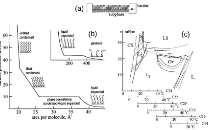
un-dergo many phase transitions. A Langmuir trough, shown schematically in (a), quasi-statically compresses a monolayer by moving a barrier that divides the fluid surface. Phase transitions in a monolayer can be identified as horizontal regions (first order transition) or kinks (second order transition) in the surface pressureπversus mean molecular surface areaAisotherms, shown schemat-ically in (b). The phase of the monolayer is controlled by the alignment of surfactant tails which is in turn controlled by the surfactant concentration and temperature. Surfactants with a similar molecular structure can exhibit similar phase transitions, for example, the phase diagram (c) of several single tailed fatty-acids, with tail lengths ranging from C-14 through C-24, exhibit similar behavior when corrected with a shift in the temperature axis. All sub-figures are from Kaganer et al.[Kag99]. . . 3 Figure 1.3 A schematic of the process of surfactant spreading on a thin viscous fluid. . . . 17 Figure 1.4 A schematic depicting the generation of meniscus waves by the vertical

(12)

Figure 1.5 There are two roots to the infinite depth dispersion relation (equation (1.51)) which correspond to gravity-capillary waveskG C W and longitudinal waveskLW of which Re[kG C W]is independent of the surface elasticity"while Im[kG C W] and Re[kLW]depend on". The complex part of the waves numbers is related to the rate at which energy is dissipated and are often called the damping factors. The value of" that corresponds to the peak in Im[kG C W]is called "maxand is the lowest value of"for which the trajectories of fluid material elements in gravity-capillary waves becomes linear (figure 1.4 (b)). These roots correspond to a fluid densityρ=1_cmg3, fluid viscosity

µ

ρ=0.01cm

2

s , and surface tensionς=70dynes_cm that are close to the values of water, and the wave oscillation frequency of_2πω =200Hz is in the capillary wave regime. This figure is adapted from Lucassen-Reynders & Lucassen[LRL70]. . . 21 Figure 1.6 The evolution of the fluid surface depicted at four evenly spaced times during

a subharmonic Faraday wave oscillation. The up and down strokes of the container are depicted with an arrow below the container. The flow field within the fluid (arrows) is significantly different from that predicted by linear gravity-capillary wave theory in figure 1.4 (b). This figure is adapted from Douady

[Dou90]. . . 26 Figure 1.7 This instability diagram, plotted for a single driving frequency, shows the

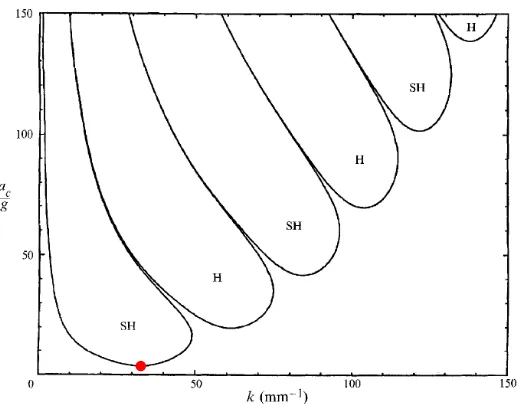
in-stability thresholds (ac_g ) for different Faraday wave modes (k) as well as the tongue-like regions that differentiate between sub-harmonic (SH) and har-monic (H) waves. Because we study a single Faraday waves mode in chapter 5, we slowly increase the driving acceleration until the first Faraday wave mode becomes unstable. Although this specific plot is derived using parameters that differ significantly from the system we study, the red dot represents a point that is analogous to the driving acceleration we use to excite a single Faraday wave mode. The location, widths, and heights of the instability tongues depend upon the fluid properties; however, in all cases there is a point (the red dot) where the onset acceleration is the lowest. When driving the system at this acceleration, a single wave mode is excited. This figure is adapted from Kumar & Tuckerman[KT94]. . . 27

Figure 2.1 The surface potential methods of measuringΓ(figure from Hühnerfuss et al.

(13)

Figure 2.2 Schematics of apparatuses for three different scanning based methods for measuring Γ. Radiotracing (a) (adapted from Sakata & Berg[SB69]) uses a Geiger-Müller (GM) tube to detect the beta emissions from the surfactant tagged with radioactive carbon-14. By scanning the scintillating tube,Γ(x,t)

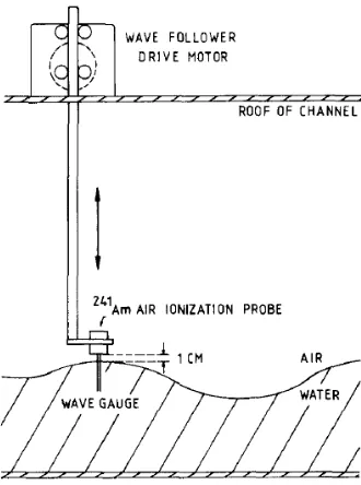
can be inferred. Second Harmonic Generation (SHG) (b) (adapted from Vogel & Hirsa[VH02]) uses surfactants tagged with special fluorophores that can up-convert incident laser light. By scanning the laser bean and the SHG detector, Γ(x,t)can be inferred. Fluorescence (c) (adapted from Bull et al.[Bul99]) uses surfactants tagged with fluorophores that can down-convert incident laser light. By scanning the laser beam, a camera can detect the emitted down-converted light which can be used to inferΓ(x,t). In both (b,c) the excitation light is

blocked by a filter placed in front of the detector. . . 31 Figure 2.3 A schematic of the original fluorescence imaging technique (a) used by Fallest

et al.[Fal10]as well as the revised apparatus (b) used in this dissertation. The basic principles are the same for both apparatuses. Surfactant fluorophores are excited by blue light and emit green light. The intensity of the camera-measured signal depends upon the concentration of the surfactant. The apparatuses de-picted in (a) and (b) use the same type of surfactant, type of fluid, and container material. (a,b) are not drawn to scale. For reference, in (b), the container’s inner radius is 14.6 cm while the distance between the camera and the fluid surface is roughly 60 cm. (c,d) sample fluorescence images (acquired through appara-tuses (a,b) respectively) during outward spreading experiments. Sub-figure (c) is taken from Fallest et al.[Fal10]while sub-figure (d) is adapted from Strickland et al.[Str14]. The experiments from which (c) and (d) are taken have the same initial mass of surfactant. The exposure time for (c) is 1 s while for (d) it is 1₄s. 34 Figure 2.4 The spectra of several material used in either the original or revised versions of

the fluorescence imaging apparatus. (a) The absorption (blue) and emission (red) spectra for NBD-PC in solution with chloroform (source: Avanti Polar Lipids, Inc.). (b) The quantum efficiency spectra for the Andor Luca-R camera used in this dissertation (source: Andor Technology, Ltd.). (c) The spectra for the black light blue lights used by Fallest et al. [Fal10](source: Koninklijke Philips N.V.). (d) The spectra for the blue LEDs (blue curve) used in this disser-tation (source: Visual Communications Company, LLC). (e) The transmission spectra for the Newport camera filter (with center wavelengthλ0=530 nm and FWHM 10 nm) used in this dissertation (source: Newport Corporation). (f ) The transmission spectra for the moiré mask filter used in this dissertation (source: Lee Filters). (g) The luminescence of anodized aluminum when excited with 305 nm light[Kom11]. . . 38 Figure 2.5 This image, taken with the Andor Luca-R camera and illuminated with blue

(14)

Figure 2.6 The non-monotonicI-Γcalibration for NBD-PC on glycerol (a) (source: Strick-land et al.[Str14]) and water (b) (source: Strickland et al.[Str15]). The calibra-tion in (a) was performed by continuous exposure while in (b), the×’s indicate continuous exposure and the’s indicate stroboscopic exposure. In all cases,

the standard deviation of the mean is smaller than the symbol size; however, for reference, the standard deviation for the stroboscopic exposure images are shown as error bars. . . 43 Figure 2.7 A schematic (a), sample data (b), and calibration (c) for the operation of laser

profilometry. This technique involves a laser that shines at an oblique angle to the surface. A camera positioned above the apparatus detects light that is diffusively reflected by the surface. The intersection between the plane swept out by the laser line and the fluid surface is proportional to the fluid depth. Sub-figures (a) and (b) are from Strickland et al.[Str14]. . . 45 Figure 2.8 The moiré imaging apparatus (a) consists of a moiré patterned light source, a

reflective fluid surface, and a camera positioned above the fluid. The reflection of the moiré mask (b) off of the flat fluid surface consists of concentric rings that alternate between opaque and transparent. (b) serves as the characteriza-tionMi j of the moiré mask. The grayscale (c) and binarized (d) reflection of the moiré pattern off of the surface wave for one phase of the Faraday wave oscillation. The sequence of eight images that (c) represents are notedDi j(tk). The detailed process of ray tracing is discussed in sections 2.2.2.1 and 2.2.2.2. 47 Figure 2.9 The position of the cameraP~, direction of the cameraκˆ, and the cm to pixel

scalingSis obtained by measuring the parallax of an array of bolts with different elevations. (a) An image of the array of bolts in grayscale with the Hough transform identified bolt heads overlaid in red. (b) An overlay showing the identified bold heads (red circles in (a)) in red and the best fit positions for the bold heads in cyan. Overlap of the red and cyan appears as white. (c) The moiré mask is characterized by imaging it through a reflection off of the flat fluid surface. The characterizationMi j is shown in the red channel. The z-position of the mask can be determined by fitting the radii of the edges between the bright and dark rings in the binarized characterization. (d)Mi j (in red) and the corresponding best fit bright rings in cyan. Overlap between the red and cyan appears as white. . . 49 Figure 2.10 The surfactant-covered gravity-capillary waves experiments in chapter 5 are

performed just above the Faraday wave onset acceleration; however, before onset, the surface profile consists of just meniscus waves. Images (a-d) show a sequence of four grayscale moiré images (Di j(tk)) for the four phases of the meniscus waves, while images (e-f ) show the corresponding best fit grayscale ray-traced pseudo-data images (Pi j(tk)). . . 53 Figure 2.11 Images (a-h) show a sequence of eight grayscale moiré images for the eight

(15)

Figure 2.12 These plots show the optimization scoreQ(equation (2.10)) vs each of the 12 fitting parameters presented in equation (2.24). In these plots,Q(B)is shown as blue curves while the value found by MATLAB’sfminsearch function is shown with a red circle. In order to highlight the behavior ofQin the vicinity of a MATLAB-found minimun, the x and y axes have been scaled to features primarily related to the minima. As a result, some of these plots appear to be cut-off. Sub-figure (k) shows a case where the optimization algorithm did not find the global minimum ofQ(B). Algorithms such asfminsearch find local minima in the vicinity of the inital guess. Because the complex multi-dimensional landscape is rough (likely a consequence of both the binarization and pixel intensity assignment process in the ray trace algorithm which rounds the intersection between the ray and the moiré mask to the next closest pixel), sub-figure (k) coincides with a local minimum. The difference between the identified local minimum and the lower minimum found along thexH Mcurve in (k) is accounted for in the uncertainty ofxH M. . . 55 Figure 2.13 The rotation rate of the Faraday wave is determined from binarized moiré

images that are taken as a set of eight (one for each phase of the Faraday wave period) for each 1 minute interval. Two binarized moiré images (a,b) taken from the same phase of the Faraday wave oscillation but spaced one minute apart bear a similar structure. The angular cross-correlation (e) can be calculated as a linear cross-correlation from the log-polar representations of the images (c,d). The angle of rotation for the Faraday wave during the 1 minute interval between the moiré images corresponds to the maximum of the cross correlation. The Faraday wave rotation rate (e) is determined for each of the eight phases (red dots), and is averaged to produce a single number used in the back rotation of the fluorescence data. . . 58 Figure 2.14 The equation of state for an NBD-PC covered fluid surface. The first

mea-surement of NBD-PC on glycerol (a) (squares) (from Bull et al.[Bul99]) was measured with the Du Noüy method. Measurements for NBD-PC on water (b) (the curve labeled b) (from Tsukanova et al.[Tsu02]) using a Langmuir trough. 60 Figure 2.15 New measurement of the equation of state for the NBD-PC covered surface

of glycerol. The three regions marked I, II, and III show regimes where the equation of state exhibits different behaviors. . . 61 Figure 2.16 (a) schematic of the shaker alignment system. Shaker response to 20 Hz

sinu-soidal signal in time (b) and frequency (c). . . 65 Figure 2.17 (a) the machine shop schematic of the aluminum well used for the wave

appa-ratus in chapter 5. The center of the well is cut to the shape of the round silicon wafer. The shape of the nose (inset) is cut to fit the notch in the wafer (b). After machining the aluminum well is anodized black. . . 66

(16)

Figure 3.2 Fluorescence intensity (proxy for surfactant concentration) measured att∗₌

5 sec, for experiments with initial conditions (a) IC6 and (b) IC4. The dashed circles (of radii 3.4 cm and 1.1 cm, respectively), highlight the corrugations in the leading edge. . . 74 Figure 3.3 The initial surface height profileh(r, 0), from equation (3.3), used in the

simu-lations. . . 75 Figure 3.4 The four equations of state used in the model, L: linear (3.4), G: Langmuir (3.6),

E: measured (3.5), M: multilayer (3.7). . . 77 Figure 3.5 Surface height profilesh(r)measured att∗₌_{5 sec in the experiment (short}

dashed lines, red), compared to numerical solutions at nondimensional times. Long dashed lines: t =2.5 (uses calculated T =2.0 sec); Solid line:t =5 (uses better-fittingT=1.0 sec). Data are from Fallest et al.[Fal10], with initial condition IC6. . . 79 Figure 3.6 (a) Surface height profilesh(r)measured att∗₌_{5 seconds in the experiment}

(dashed lines) andt=5 in numerical solution (solid line); the locationr=rM of the peak is marked with a•. (b) The corresponding surfactant concentration profilesΓ(r)in the experiment (noisy) and numerical solution (smooth); the locationr =r0of the leading edge of the surfactant is marked with a•. Data are from Fallest et al.[Fal10], with initial condition IC6. Note that the larger scatter near the origin is due to the decreasing number of pixels over which the average is taken. The small peak inI(r)near the leading edge arises due to fluorescence resonance energy transfer (FRET) between nearby fluorophores

[Shr95]. As a result of FRET, the relationship between fluorescence intensity and surfactant concentration can exhibit non-monotonic behavior[Str14]. . . 80 Figure 3.7 Comparison between spreading rates of (a) the location of the maximum of the

surface height profileh(r)and (b) the location of the leading edge of surfactant in both experiment and simulation. Colored curves are from experiments with IC6 adapted from Fallest et al. 2010, black dots are from simulations. Dashed curves are (a) comparison to best-fittαwithα=0.295 and (b) comparison to

t1/4. . . 81 Figure 3.8 Azimuthally-averaged fluorescence intensity (in arbitrary units specific to our

Andor camera) at a distancer from the center of the surfactant region, shown at representative times, taken from an experiment with IC4 ( ¯Γ∗₀<Γc). . . 82 Figure 3.9 Images comparing the laser profile for two experiments with IC5 (a-e) ( ¯Γ∗₀>Γc)

and IC2 (f-j) ( ¯Γ∗₀<Γc) at five different times. The uppermost bright line in each image is the reflection from the air-glycerin interface, and is used to measure the free surface height profileh(t). . . 83 Figure 3.10 The spreading dynamics of the location of the leading edge of the fluorescence

intensity (r0), scaled by the ring radiusR0. The dashed lines corresponding to

t1/4andt1/10spreading behavior are shown for comparison. . . 84

(17)

Figure 4.2 Self-healing of surfactant layer. Sample fluorescence imaging (FI) and laser profilometry (LP) images forΓ0=0.8Γc,H=0.7 mm, andR=3 cm. The bright horizontal laser sheet reflection measures the height profileh(r,t), and the background intensity measures the surfactant concentrationΓ(r,t). The time series of a typical experiment starts when the retaining ring is lifted (a), after which the capillary ridge travels inward and forms the vertical distension as the central surfactant-free (dark) region shrinks (b−d). At timetmax, the distension reaches its largest size (e) and then decays (f). The position of the maximum of the Marangoni ridge is denoted byrM and the position of the leading edge of the surfactant is denoted byrS. . . . 93 Figure 4.3 Calibration data relating surfactant concentrationΓto fluorescence intensityI.

Because the curve is non-monotonic, we use a piecewise linear fit (regions A, B, C) to the empirical data. Error bars (standard deviation of the mean intensity) are smaller than the points. . . 94 Figure 4.4 The equation of state used in the simulations (Eqn. 4.4). The equation of state

relates the nondimensional surface tension ˜σto the nondimensional surfac-tant concentration ˜Γ. . . 97 Figure 4.5 Typical numerical simulations with growth and decay of fluid and self-healing

of surfactant. Redimensionalized numerical simulations of Eqn. 4.1 and Eqn. 4.2 usingΓ0=0.8Γc,H=0.7 mm, andR=3 cm (the same parameters as in Fig. 4.2). In each panel, the surface representsh(x,y,t)and the color of the surface ranges fromΓ =0Γc(black) toΓ =1Γc (green). The insets highlight the shape ofh(y)cut through the center of the surface plots. The simulation starts from (a) the initial film height and surfactant concentration, and the resulting dy-namics are (b) the formation of the distension as the annular Marangoni ridge coalesces toward the center of the region. At timetmax, the distension reaches its largest size (c) and then decays (d). Times have been redimensionalized byT/α0.8, as will be discussed in §4.4, to permit a direct comparison with the

experiments. . . 99 Figure 4.6 Distension growth and decay. Dynamics are captured by tracking heighthc at

the center of the system. Experiments (filled symbols) and redimensionalized simulations (open symbols) at five different initial surfactant concentrations. For reference, the gray dotted curve shows the 1.0Γc simulation without theα rescaling. As discussed in §4.3.2, simulation times have been redimensionalized and then further reduced by a factorα0.2=17.2₋+_0.012,α0.4=7.81±2,α0.6= 6.07±1,α0.8=11.0±1, andα1.0=9.91±2, respectively, where the±values represent the uncertainty inα. . . 101 Figure 4.7 Distension growth dynamics. (a,c) Experiments (solid) and (b,d)

(18)

Figure 4.8 Kymograph of the surfactant concentration profile for the 0.6Γc experiment. Surfactant propagates outward in the region demarcated by the two white dashed lines. The color scale is truncated at 0.55Γcand 0.75Γcin order to isolate the region of interest. For reference, the maximum surfactant concentration within the green colored saturated region is 1.4Γc. . . 103 Figure 4.9 Maragoni ridge and surfactant leading edge dynamics. (a) The peak of the

Marangoni ridge (rM) and (b) the inward motion of the leading edge of the surfactant (rS) at five different initial surfactant concentrations, for both ex-periments (solid lines) and redimensionalized simulations (dashed lines). For the experiments, all locations are determined by visual inspection of theh(r,t)

andΓ(r,t)profiles. In the simulations,rSis the first point where the surfactant concentration rises above 0.001Γc; choosing a lower threshold does not signifi-cantly affect the results. In all cases,R=3.0 cm andH=0.7 mm; the horizontal dotted line indicates the initial ring location atr =R. The closing timetc is defined as time at whichrS =0; in the experiments, this is found by visual inspection of the images. (c) The position of the leading edge of the surfactant (same data asa), but plotted as a function of (tc−t) to permit comparison to the asymptotic solution from Jensen[Jen94a](black line). The symbols identify the initial conditions used for each curve. . . 105 Figure 4.10 Profiles attmaxfor range ofΓ0. (a,b) Fluid height and (c,d) surfactant

concen-tration profiles for FI/LP experiments and redimensionalized simulations at timetmax, starting from five values ofΓ0withR=3.0 cm andH=0.7 mm. (a,

c) Experiments and (b,d) simulations are plotted in solid and dashed lines re-spectively. Vertical dotted lines indicate the initial ring location atr=R. From lowest to highestΓ0,tmaxis 12.08, 11.25, 9.02, 3.60, and 3.21 (s). The symbols identify the initial conditions used for each curve. . . 106 Figure 4.11 Distension decay dynamics. (a,c) Experiments (solid) and (b,d)

redimension-alized simulations (dashed) of distension decay dynamics for initial conditions Γ0=0.6Γc,R=3 cm, andH=0.7 mm. Height profileh(r,t)(a,b) and surfac-tant concentration profileΓ(r,t)(c,d) at representative times during decay. Vertical dotted line indicates the initial ring location atr=R. . . 107 Figure 4.12 Power law decay nearΓc. Comparison of experiments (solid lines) and

redi-mensionalized simulations (dashed lines) at three values ofΓ0, highlighting the distension decay dynamics using data from Fig. 4.6. The simulation curves account for the meniscus by adding the experimentally-observed hm a x = 0.36 mm, measured in a ring-lifting experiment when no surfactant was present. The solid line is a comparison to a power law decay with exponent−1/3, pro-vided for comparison. The symbols identify the initial conditions used for each curve. . . 108 Figure 4.13 Dependence of distension sizehmaxon geometric parameters. LP experiments

with a bulk concentration of PDMS. (a) For fixedR=1.5 cm and varyingH

(second row of Table 4.2), with〈hmax〉=0.86 mm (dashed line). (b) For fixed

(19)

Figure 4.14 Dependence of distension sizehmaxon material parameters. Simulations (open symbols) and both FI/LP and LP experiments (closed symbols). (a) Experi-ments and redimensionalized simulations with a variety of initial concentra-tions of NBD-PC and fixedH=0.7 mm andR=3.0 cm (first row of Table 4.2). (b) Experiments on five surfactant types, with fixedR=1.5 cm,H=2.0 mm, andV=540µL (fourth row of Table 4.2).σ0−σSquantifies the surface tension contrast for each surfactant. Dashed line is〈hmax〉=1.12 mm. . . 109

Figure 5.1 Experimental apparatus. The container (black) is connected by low-friction air bushings to an electromagnetic shaker, and filled with a thin layer of water onto which a monolayer of NBD-PC surfactant is deposited. The shaker vibrates the container vertically with accelerationa(t) =a0sinωt, generating meniscus and Faraday waves. The fluorescence imaging system involves a ring of blue LEDs around the outer edge that excites the fluorophore on the lipids; digital images of the fluorescence emission are collected through an optical notch filter. A silicon wafer sits flush with the bottom surface of the container, and reflects the excess light from the LEDs away from the camera. The moiré imag-ing system consists of a patterned light source shinimag-ing downward on the fluid surface, and the camera which records the distorted reflection of the pattern. 116 Figure 5.2 Stroboscopic imaging allows for the collection and phase-averaging of

low-intensity fluorescence images over many cycles. During each second of the experiment, the container oscillates 20 times with an accelerationa(t)(black curve). During that second, the camera is triggered at four different phases of the oscillation (eight different phases of the Faraday wave oscillation). The eight distinct phases (represented asi=1 throughi=8) each have an exposure time of 1/8 of the Faraday wave period, represented by the width of the gray bars. The time from the end of one exposure to the beginning of the next exposure is one whole Faraday wave period (100 ms), so that we sequentially sample each of the eight phases cyclically. The same stroboscopic pattern was used for both experiments, and both the FI and MI data. . . 119 Figure 5.3 Calibration of surfactant fluorescence intensity as a function of surfactant

(20)

Figure 5.4 Sample FI composite image (a) showing∆Γfrom thei=2 stroboscopic phase of Experiment 1, smoothed by a Gaussian filter ofσ=0.04 cm. (b) The corre-sponding∆ΓT, the best fit to (5.2). (c) The meniscus wave (harmonic) com-ponent and (e) the Faraday wave (subharmonic) component of the same∆Γ shown in (a). These components are isolated by adding and subtracting (and dividing by 2) the FI composite images from thei=2 andi=6 stroboscopic phases. (d) The meniscus wave (harmonic) component and (f) the Faraday wave (subharmonic) component of the same∆ΓTshown in (b). (g) This im-age is generated by subtracting (d) from (c). The resulting pattern (smoothed with a Gaussian filter ofσ=0.09 cm) is a higher-order mode which is not ac-counted for in the ansatz (5.2). This mode has 24-fold symmetry and oscillates harmonically with peak-to-mean variation of 0.03Γc. . . 123 Figure 5.5 Sample MI images. (a) Contrast-enhanced image and (b) binarization of the

target pattern reflected off a flat fluid surface. (c) Contrast-enhanced moiré image and (d) binarization of the target pattern reflected off the fluid surface at phasei=2 for Experiment 1. (e) Ray-traced pseudo-image and (f) binarization of the best-fith(r)for image (c) using parameters given in table 5.1. . . 124 Figure 5.6 Visualization of∆hT and∆Γfor Experiment 1, within the annular field of view.

The best fit using theh-ansatz (5.1) (mesh surface) and the FI composite data (colouration) for thei=2 stroboscopic phase. The peak-to-mean variations in ∆hT and∆ΓT are±60µm and ±0.15Γc respectively. The∆Γfields are smoothed by a Gaussian filter ofσ=0.04 cm to reduce noise. In figures 5.7 and 5.8, this same data is decomposed into its meniscus and Faraday wave components. . . 129 Figure 5.7 Meniscus wave component of∆hT and∆Γfor Experiment 1. (a) The best

fit∆hM T ansatz from (5.1) (mesh surface) and the harmonic component of ∆Γ(colouration) for thei =2 stroboscopic phase. (b) Radial slice of both fields alongθ =2.83 radians, the orange strip shown in (a), at phasei =2. The solid line is the best-fit height field∆hM T(r), and the surfactant density field is shown both as the data∆ΓM(orange points) and as the ansatz∆ΓM T (dashed line). The lines are the Bessel modes given in (5.1) and (5.2). (c) The temporal dynamics of∆hM T (solid line) and∆ΓM T (dashed line) at the location

(21)

Figure 5.8 Faraday wave component of∆hT and∆Γfor Experiment 1. (a) The best fit

hF T ansatz from (5.1) (mesh surface) and the sub-harmonic component of∆Γ (colouration) for thei=2 stroboscopic phase. (b) Radial slice of both fields alongθc=2.83 radians, the orange strip shown in (a), at phasei=2. The solid line is the best-fit height field∆hF T(r,θc), and the surfactant density field is shown both as the data∆ΓF (orange points) and as the ansatz∆ΓF T (dashed line). The lines are the Bessel modes given in (5.1) and (5.2). (c) Azimuthal slice of both fields alongrc =4.26 cm, the cyan strip shown in (a), at phase

i =2. Here, the surfactant density field data∆ΓF is represented with cyan points. The lines are the sinusoids given in (5.1) and (5.2) and plotted within a restricted range of the azimuthal dimension−2π_n ,2π_ncentered aboutθc. (d) The temporal dynamics of∆hF T (solid line) and∆ΓF T (dashed line) at the locationrccm andθc radians, marked by the magenta dot in (a). The lines are the sinusoids given in (5.1) and (5.2). The magenta circles in (d) plot behavior ofT(t)given in (5.3), with errorbars much smaller than the symbol size. The ∆Γfields in (a,b,c) are smoothed by a Gaussian filter ofσ=0.04 cm to reduce noise. . . 131

Figure 6.1 Experimental apparatus. The container (black) is is filled with a thin layer of water onto which a monolayer of NBD-PC surfactant is deposited. The container is connected to a shaker which vibrates the container vertically with an acceleration ofa(t) =a0sin(ωt), generating meniscus and Faraday waves. The camera images a reflection of the ring flash. In the presence of Faraday waves, the reflection is significantly distorted; however, if the surface has only meniscus waves, the reflection is minimally distorted. . . 140 Figure 6.2 The algorithm for finding the Faraday wave onset involves examining the

images of the distorted reflection of the ring flash for different driving accelera-tion amplitudes. Once the Faraday waves onset, the reflecaccelera-tion of the ring flash (undistorted in (b)) becomes distorted (c). Consequently, the number of bright pixels in the image significantly increases. The reported onset acceleration (red dot) is the lowest acceleration ampiltude at which the Faraday waves are visible. 141 Figure 6.3 Onset acceleration vs driving frequency for several different initial

concen-tration of the NBD-PC surfactant on water. The data (solid symbols) use four different initial concentrations of NBD-PC. The predictions (lines with open symbols) use equation (6.1) for three of the four surfactant concentrations. . . 144 Figure 6.4 Onset acceleration vs surfactant concentration for a 70 Hz driving frequency.

(22)

Figure A.1 There are two principal modes of deformation in a bulk material element. In dilation, a finite material element is stretched or shrunk along its principle axes. In pure shear, the material element is stretched along one diagonal while being shrunk along the others. The cyan coloration of the above figures indicates the new volume occupied by the material element while the red coloration indi-cates the volume that the element has lost. White shows the overlap between the original state of the material element and the state post deformation. This figures is adapted from Mayer & Eliassen[ME71]. . . 173 Figure A.2 There are four principal deformation modes for a surface material element.

Dilation and shear have already been discussed in §A.1.3 and figure A.1 but are repeated here for completeness. In bending, the material element bows in such a way that the center point moves normal to the element further than the corners. In torsion, the material element forms a saddle, and the center point remains stationary. The coloration used in the lower set of figures differs from that used in the upper figures. Cyan indicates regions where the deformed surface material element is above the undeformed element whereas red indicates the opposite. This figures is adapted from Mayer & Eliassen

(23)

CHAPTER

1

INTRODUCTION

1.1 What are surfactants?

Fluid mechanics assumes that fluid materials are fundamentally continua. For problems involving

macroscopic bulk flow, this assumption is justifiable because the length scale of molecular

interac-tions is much smaller than the length scale of the continuum dynamics. Surfaces, however, behave differently. There is a broken symmetry at the surface: the material on one side is different than the

ma-terial on the other side. Consequently, molecular-scale chemical interactions, which would otherwise

be subsumed into a fluid’s bulk constitutive relation, have macroscopic effects. Transitioning from the molecular-scale to the continuum scale, the discrete molecule effects are coarse grained to give

an effective surface tension. The surface tension acts to minimize surface area while simultaneously

inducing a discontinuity in the pressure field at the interface.

For uncontaminated fluid interfaces, this treatment works well, but when a SURFace ACTive

AgeNT (surfactant) is present, the bulk fluid dynamics are coupled to the dynamics of the surface

contaminant. By changing the chemistry of the interface, surfactants can reduce the surface tension in a way that depends upon the surface density of the surfactant. Further, motion and deformation

of the surface is complicated by interactions between the surfactant molecules. Consequently, the

dynamic properties of a surfactant monolayer cannot be fully characterized by an effective surface tension.

(24)

1.1. WHAT ARE SURFACTANTS? CHAPTER 1. INTRODUCTION

(a)

(b)

(c)

(d)

(e)

(f)

hyd

rop

ho

bi

c

tai

ls

hydrophyllic heads

Figure 1.1: The microscopic perspective of a surfactant-covered interface. (a) the molecular model of DPPC (Dipalmitoylphosphatidylcholine), the largest constituent of pulmonary surfactant and a commonly studied molecule (Avanti Polar Lipids); (b) the molecular model of an NBD-PC molecule, a molecule we will study in this dissertation (Avanti Polar Lipids); (c) the molecular model of wa-ter (reproduced under the Wikimedia commons license); and (d) the molecular model of glycerol (reproduced under the Wikimedia commons license), all roughly to scale. (e) The surface of clean water[Jun11]is roughly 1-molecule deep, and the dangling Hydrogen-bonds give rise to a surface energy known as surface tension. (f ) A snapshot during a molecular-dynamics simulation of the DPPC covered water surface[MA10].

a hydrophylic headgroup (a polar chemical group) with one or many hydrophobic tails (a

non-polar chemical group, typically hydro-carbon or fluoro-carbon chains) (figure 1.1 (a,b) )[Lan17b; Lan17a; Lan20]. The polar head groups are attracted to the hydrogen bonds between water (or

glycerol) molecules and, when dissolved in water, participate in hydrogen bonding with adjacent

water molecules. The non-polar tails, however, do not participate in hydrogen bonding and, when dissolved in water, restrict the orientational freedom of neighboring water molecules. This reduction

in the orientation freedom of the water molecules results in a net decrease in entropy[Sil98]. At the surface, hydrogen bonds are exposed (figure 1.1 (c,d,e)) such that the introduction of

the polar head group reduces the surface energy. Because of the asymmetry of the amphiphilic

molecules, the surfactant will self-assemble into a surface film that is a single molecule thick (figure 1.1 (f )). Depending upon the length of the hydrophobic tails, some types of surfactant molecules

will desorb from the surface into the bulk (or reciprocally absorb from the bulk to the surface). Long

hydrophobic tails serve as a greater entropic barrier and thereby reduce the solubility of the surfactant in the sub-phase[Sil98]. Consequently, monolayers are often divided into two categories: Langmuir

monolayers (insoluble) and Gibbs monolayers (soluble). For Langmuir monolayers, the dynamics are

(25)

(b)

(a)

(c)

(26)

chemical (i.e. adsorption/desorption). Although there are additional types of dynamics that could be

categorized as chemical (such as reactions that change the chemical species of the surfactant), we will consider Langmuir monolayers, thereby focusing on the mechanics of the monolayer.

On the equilibrium coarse-grained continuum scale, the surfactant layer behaves like a

2-dimensional compressible material with, in some cases, a significant bending modulus[Wax84; Lan14]. Through quasi-static compression of the contaminated surface (figure 1.2 (a)), surfactants

can undergo various phase transitions and, in analogy to the commonly known states of matter

for 3-dimensional materials, can change phase from a 2-dimensional gas to a liquid to a solid etc. The equation of state (figure 1.2 (b,c)) for a surface material relates the ambient temperatureT, the

surfactant densityΓ, and the surface pressureπ. The pressure of the surface material is determined from the surface tensionςand is calculated asπ(Γ) =ς0−ς(Γ)whereς0is the surface tension of the

uncontaminated sub-phase[Kag99]. As originally noted by Agnes Pockels[RP91], the isotherm of

these materials exhibits two different behaviors depending on the surface density of the surfactant. When the surfactant density is low,ςdecreases with increasingΓ; however, when the surfactant density exceeds the critical monolayer densityΓc,ςremains constant. When the surfactant density is belowΓc, the surfactant material forms monolayers[Ray99; Kag99]; however, when compressed beyondΓc, the material collapses out of the surface and forms a multi-molecule thick film.

In dynamic processes, the presence and mechanical properties of a surfactant monolayer can

significantly change the motion in the bulk fluid. Pliny the Elder[Pli]and Aristotle[Ari]noted the effect of oil on water observing that pearl divers, when under water, would release oil from their mouths

so that the surface waves would be stilled and light could shine to the murky depths for the divers

to see. Franklin et al.[Fra74]additionally noted that the use of oil could save ships in violent storms, a suggestion that was applied successfully to Arberdeen harbour[Ait82]. The current perspective,

derived from observations of Marangoni[Mar70]and Boussinesq[Bou13], holds that the surfactant

can undergo compression and shear. Inhomogeneous compression of the surface phase will generate surface pressure gradients (or surface tension gradients) which are called Marangoni stresses. In cases

where gradients in the surface velocity are significant, the compression and shear viscosities of the

surface generate additional stresses. When the surface of a fluid is contaminated with a surfactant, the stresses that perturb the monolayer are balanced by the bulk fluid’s excess surface stress. Then,

through viscosity or elasticity, the effects of the surfactant propagate into the material’s bulk and

change the bulk flow.

Surfactants are used in a plethora of industrial and biological processes, of which we will make

reference to two: pulmonary surfactant therapy, where pulmonary surfactant is administered to

(27)

1.2. MOTIVATING QUESTIONS CHAPTER 1. INTRODUCTION

where a monolayer of surfactant spreads on a thin viscous fluid mimics the delivery process of

pulmonary surfactant which spreads on pulmonary mucous. Similarly, our experiments of surfactant covered gravity-capillary waves mimics the interaction between oil slicks and ocean waves.

1.2 Motivating questions

Although the macroscopically static surfactant-covered interface is well understood, the interfacial

dynamics on a macroscopic scale are not. Throughout this dissertation, we will repeatedly raise the

question: what are the spatio-temporal dynamics of an insoluble surfactant monolayer? There are many studies that examine dynamic processes that involve surfactants[Lan98; ZT05; Bra12; GG96;

LRL70; Zan02; CF95; CM09; Pug96; Dre07; Rei09; Sol05; Zha03]. Of these studies, many infer the

dynamics of the surfactant layer based on the motion in the bulk phases. To answer the question in the strictest sense, we must report the spatio-temporal dynamics of the surfactant directly (i.e.

measuringΓ(~r,t)). There are five established techniques for doing this, which we will discuss in detail in chapter 2; however, none of these techniques measuresΓover both surface coordinates and time. Typically at lest one[SB69; GS72; WN78; Vol80; AN88; Vog01; VH02; BM89; Bul99; BG03; Fal10](if not

both[Hüh85]) of the surface coordinates are omitted and sometime the temporal behavior as well

[BM89]. Additionally, these techniques are cumbersome and most have poor temporal resolution. In this work, we will present an enhancement of a fluorescence imaging technique (originally

developed by[Fal10]) for measuringΓ(~r,t)that allows us a spatio-temporal characterization ofΓwith a temporal resolution of at leastO(0.01 s). We will present the details of this method in chapter 2, and we will demonstrate the efficacy of this method by studying the spreading of a surfactant on a thin

viscous fluid (chapter 3), the self-healing of a surfactant monolayer on a thin viscous fluid (chapter 4),

and the perturbation of a surfactant monolayer by gravity-capillary waves (chapter 5). Each of these studies bears scientific interest in its own right.

1.2.1 Surfactant spreading and self-healing

Surfactant spreading is, historically, the quintessential dynamic study of surfactants as surface layers. Based on qualitative tests, Franklin et al.[Fra74]noted that surfactants on water spread to cover the

fluid surface; however, they inaccurately attributed this to a repulsive effect within the surfactant

material when on the surface of water. Thomson[Tho55], noting a similar effect wherein tracer powder on the surface of water would move outward after the deposition of a droplet of alcohol,

postulated that surface tension gradients drove the dynamics and the transport of the surface material,

(28)

Since Rayleigh[Ray99]noted that surfactants form mono-molecular films, the studies of a

sur-factant spreading can be divided into into the spreading of a bulk sursur-factant film[HF22]on a fluid surface and the spreading of a monolayer[CR25]; and further sub-divided into the case of a deep

fluid layer[Fay71]and a thin fluid layer (where lubrication theory is valid)[GG92]. In this latter case

of spreading on a thin fluid layer, Levich[Lev32]derived a formalism, corrected by Yih[Yih68], for the dynamics of the fluid bulk and the surface morphology as driven by surface tension gradients.

This formalism assumes steady flow and a steady surfactant distribution so as to decouple the fluid

dynamics from the surfactant dynamics. Using this formalism, Ahmad & Hansen[AH72], without considering a full theoretical characterization of the transport of surfactant, argued that the distance

traveled by a linear spreading front (in Cartesian coordinates) isx∼t1/2and conducted experiments with oleic acid spreading on glycerin that supported their prediction.

Borgas & Grotberg[BG88]developed a theoretical framework that included surfactant transport

(advection and diffusion intended for the case of a surfactant monolayer) by the underlying steady flow. This framework included the effects of capillarity, gravity, and surface viscosity in addition to

the Marangoni and bulk viscous effects. From this treatment, Gaver & Grotberg[GG90]developed

a set of two coupled PDEs that modelΓandh that accounts for capillary, gravity, Marangoni, and bulk viscous effects. This model (which we will derive in §1.4.1) has become a touchstone for ongoing

work concerning the dynamics of surfactant on thin fluid films including pulmonary drug delivery

[GG90], surfactant replacement therapy[GG92], ocular surfactants and blinking dynamics[Bra12; Mak10], spreading of soluble surfactants[JG93; HG92], solute transport[Jen94a], latex paint drying

[Eva00; GR06; Gun08], ink-jet printing[Han11], secondary oil recovery[Han12; Sin11], the spreading of exogenous into endogenous surfactant[Esp93; Gro95; Bul99], self-similarity analysis of the surfactant spreading problem[JG92; Jen94a], and studies of the jump condition at the surfactant leading edge (a

shock front) Shearer & Levy[SL06]; Levy et al.[Lev07]; Peterson[Pet10]; Peterson & Shearer[PS11];

Peterson & Shearer[PS12].

The popularity of the Gaver & Grotberg[GG90]model indicates its utility; however, the model has

not been subject to a rigorous examination of its predictions concerning bothhandΓfor monolayer spreading. Until recently, there have been only four experimental tests of the model[GG92; Bul99; BG03; Dus05], all of which have only studied surfactant spreading systems where the initial surfactant

concentration is grater thanΓc. These studies have also only considered two quantities,h(~r,t)and the surfactant leading edgerΓ, leaving the predictions aboutΓ(~r,t)untested. The combined efforts of Fallest et al.[Fal10]; Swanson et al.[Swabl]have produced a fifth test of the model’s predictions

concerningΓ(~r,t)when the initial surfactant concentration significantly exceedsΓc.

(29)

monolayer concentration of oleic acid spreading on glycerol) used a colored tracer fluid to detect the

advancing surface compression front. The apparatus consisted of a spreading solution, consisting of hexane and oleic acid, deposited on the surface of glycerin within a containing ring such that after

the hexane spreading solvent evaporated, the ring was lifted and the experiment commenced. These

methods quantitatively agreed with the model’s predictions for the compression frontrc f −1∼tα whereα≈0.7.

Using an apparatus similar to Gaver & Grotberg[GG92], Bull et al.[Bul99]further tested the model

by studying the leading edge of near-monolayer concentrations of fluorescence NBD-PC spreading on glycerin into a monolayer of pre-existing PL-PC and claimed quantitative agreement with the model

predictions of(r_Γ∗−r0)/r0=1.02t0.59wherer0is the radius of a containing ring that separated the NBD-PC from the PL-PC.

Dussaud et al.[Dus05]considered a drop of pure oleic acid spreading on a thin glycerol film

without the use of a retaining ring, and found that the minimum in the gradient of the fluid height profile traveled outward at a rate ofR∼t1/4while the maximum gradient travels asR∼t0.15_{. Dussaud}

et al.[Dus05]found that agreement with the theory was possible, provided that the models have a

small initial amount of surface contaminant.

Fallest et al.[Fal10]considered an apparatus similar to Bull et al.[Bul99]except without the PL-PC

surfactant outside of the containing ring, and with the ability to conduct fluorescence imaging and

height profilometry thereby directly testing the predictions of the model. Fallest et al.[Fal10]found that the peak of the Marangoni ridge and the surfactant leading edge are roughly coincident and

spread at a rate of nearlyrΓ∼t1/4. Swanson et al.[Swa13], continuing the analysis of the data by Fallest et al.[Fal10], found that the predicted height profiles qualitatively agreed with the predictions but that the time redimensionalization and the surfactant concentration profiles do not agree.

Amidst all of these works, there remain several open questions. What are the dynamics of a

monolayer spreading (chapter 3)? Do the predictions of the Gaver & Grotberg[GG90]model become more accurate when considering the spreading of a monolayer of surfactant (chapter 3)? In context

of the fact that the geometry of the surfactant front affects the dynamics (e.g. a planar Cartesian

front spreads asx∼t1/2while a cylindrical front spreading asr_Γ∼t1/4), what are the dynamics of a cylindrical front spreading inward (chapter 4)? This inward spreading system can be understood as

the inverse of the outward spreading system studied in previous tests of the Gaver & Grotberg[GG90]

model. Surfactant can be deposited on the outside of a retaining ring such that once the system equilibrates, the area within the ring remains surfactant-free. Upon lifting the ring, the surfactant

spreads inward due to Marangoni stresses. In this inward spreading geometry, can the Gaver &

(30)

In chapters 3 and 4, we will consider the spreading of a monolayer of NBD-PC surfactant on a

thin layer of glycerol. In chapter 3, we will study the outward propagation of a cylindrical front. We will initiate the dynamics by depositing the surfactant inside of a retaining ring such that once the

surfactant reaches equilibrium within the ring, we will slowly lift the ring leaving behind a circular

patch of surfactant that will spread outward. In chapter 4, we will consider the inverse geometry where a cylindical front will spread inward tor =0. In this second case, we will initiate the dynamics by depositing the surfactant outside of the retaining ring such that once the ring lifts off of the surface, an

annular patch of surfactant will spread inward covering the circular vacancy at the origin. In §2.4, we will question the assumed equation of state used in the simulations of chapters 3 and 4, and we will

present new measurements of the equation of state for NBD-PC on glycerol. In §7.1, We will discuss possible implications and future work regarding the new measurements of the equation of state.

1.2.2 Surfactant-covered linear waves (meniscus waves)

The influence of a surfactant on gravity-capillary waves has been known since antiquity[Pli; Ari; Fra74;

Ait82]and has been used to eliminate the waves during stormy ocean conditions. A robust account of this mechanism was not offered until the early twentieth century, when, independently, Levich

[Lev41a; Lev41b]; Dorrestein[Dor51]; Goodrich[Goo61a; Goo61b]developed a linearized theory to describe the dynamics of surfactant-covered gravity-capillary waves in a Cartesian geometry. These theoretical works show that the presence of a surfactant increases the dissipation of energy as the

wave propagates. As a result, the waves decrease in amplitude.

Both theoretical predictions and experiments concerning these Cartesian waves show that the surface morphology is∆h=Aei(k x+ωt)_{. Similarly, the linear waves in a cylindrical geometry}_[_Boc91; Say00; PD06](which we will consider in §1.4.2 and chapter 5) have a surface morphology that follows ∆h=A J0(k x)eiωt. In either case, the linear theory predicts that these waves compress and expand different regions of the surface. If the surface is surfactant free, this compression/expansion of the

surface does not induce surface stresses, and the waves lose energy slowly owing to bulk viscous damping; however, when a surfactant is present, these variations in the surface area do generate

surface stresses which in turn dissipate a considerable amount of energy through a viscous boundary

layer near the surface. This linear theory predicts, in agreement with experiments[DV65; LH66; Fis85], that the damping factor depends upon the surface rheology (the stress-strain-rate relation

for the surface which, when linearized, is characterized by the surface compressibility"= Γ0_ddς_Γ, the surface dilational viscosityΛ, and the surface shear viscosityM). Because the damping factor can be determined experimentally as the complex part of the wave number and related to the rheology of the

(31)

in particular the dilational surface viscosity, from measurements of∆h[Miy83; Jia93; Say00; Beh07; Mon07].

Lucassen[Luc68a]observed that the dispersion relation for these surfactant-covered

gravity-capillary waves permits a second physically meaningful solution. This second type of wave (often

called a longitudinal or Marangoni wave), exhibits significant horizontal motion of the surface with minimal vertical motion. Observing that the maximum in the damping factor coincides with the

equality between the real parts of the gravity-capillary and longitudinal wave numbers, Lucassen

[Luc68a]postulated that surfactant-covered gravity-capillary waves can resonantly excite longitudinal waves. Inspired by this prediction, Budach & Möbius[BM89]conducted a series of experiments

looking for the resonance assuming that any perturbation of the surfactant distribution correspond to a longitudinal waves. Using a Förster resonance energy transfer based method wherein a fluorescent

surfactant is excited with a mercury lamp and emits light of a larger wavelength, Budach & Möbius

[BM89]measured∆Γand∆hover a single surface coordinate and at a single phase of the wave oscillation. Budach & Möbius[BM89]reported that the peak in the gravity-capillary wave damping

was roughly coincident with the maximum in the amplitude of the surfactant distribution; however,

Budach & Möbius[BM89]did not report any other information (spatial or temporal) about∆Γ. Since these experiments, Ermakov[Erm03]has shown that, within the Lucassen[Luc68a]formalism, the

solenoidal component of the bulk flow behaves like a longitudinal wave. Further, the solenoidal

component achieves a maximum amplitude at the same surface elasticity that gives the equality between the real parts of the gravity-capillary and longitudinal wave numbers.

Despite this assortment of theory and experiments, surprisingly little attention has been given to ∆Γ. The majority of the theoretical considerations do not refer to∆Γat all but instead consider the related quantity∆_AA=dξ_dx whereAis a unit of surface area[LRL70]andξis the horizontal displacement of a material element of the surface. Only recently did Picard & Davoust[PD06]produce a prediction

for the spatio-temporal dynamics of∆Γ; however, for lack of solving the dispersion relation, they did not predict the relation between∆Γand∆h. To date, the best prediction about this relationship must be inferred from Lucassen-Reynders & Lucassen[LRL70]who, studying these waves in Cartesian

coordinates, qualitatively described the relationship betweenξand∆has a temporal phase shift. As "increases from 0 to the value that corresponds to a maximum in the damping factor, the phase shift increases fromπ₂ toπ, and as"→ ∞, the phase shift remains constant whileξ→0. Using the fact that

∆A A =

dξ dx =−

∆Γ

Γ , the relation between∆Γand∆htakes the from of a temporal phase shift that varies from 0 toπ₂ depending upon". We will consider the relation between∆hand∆Γin more detail in §1.4.3.

(32)

linear wave theory predict the dynamics of∆Γ?

In chapter 5, we will study the propagation of gravity-capillary waves in water covered with a monolayer of NBD-PC. By vertically shaking the meniscus, we will produce cylindrical gravity-capillary

waves within a cylindrical container. These meniscus waves obey the linear theory predictions for∆h

[Say00; PD06; PD07]and will allow us to study the relationship between∆Γand∆h.

1.2.3 Surfactant-covered Faraday waves

Faraday waves, first observed by Faraday[Far31], are excited by the vertical shaking of a fluid. These

waves form when the driving acceleration exceeds the onset acceleration (also called critical or threshold acceleration), which is determined by the balance between the energy injected into the

system through the driving acceleration and the energy dissipated through viscous effects. Faraday

waves differ from meniscus waves in two key aspects. First, the energy injection for meniscus waves comes from a contact line whereas for Faraday waves, the energy is injected through the entire bulk

material. Consequently, meniscus waves are traveling waves while Faraday waves are standing waves.

Second, for linear waves, a sinusoidal excitation generates a disturbance with a single well-defined wavelength. For Faraday waves, the modulation of gravity can result in the superposition and coupling

between many different surface modes. As a result, the Kelvin dispersion relation does not apply to

Faraday waves[Kum96]. Depending on the fluid properties and parameters of the driving acceleration, Faraday waves can either oscillate harmonically (with a period equal to the driving period)[Mat70;

Mül97]or sub-harmonically (at twice the driving period)[Ray83; Mül97]. Faraday waves have been a

source of fascination in the non-linear dynamics community because of the wide array of patterns that the waves form[EF94; Wag03]and the many modes of symmetry breaking that can lead additional

instabilities and ultimately chaos[GM83; CG84; Gol06].

A standard approach to predicting the onset acceleration and wave pattern at onset is by assuming that the surface morphology is a superposition of normal modes and considering, via linear-stability

analysis, the stability of each mode at a given driving frequency and amplitude[BU54; KM04b; KM04a; Kum96; KM02a; KT94; SK08; KM02b; Mat04]. As the driving acceleration is increased above the onset

acceleration, multiple wave modes can interact resulting in the symmetry breaking effects that lead to

chaos.

As we will discuss in more detail in §1.4.3, the study of surfactant on Faraday waves has followed

several different routes. Experiments by Henderson et al.[Hen91]; Henderson[Hen98]studied the

en-ergy dissipation induced by the presence, type, and concentration of a surfactant monolayer. These ex-periments showed agreement with the damping rates predicted by Miles[Mil67]and consistency with