Seismic Hazard Analysis based on the Joint Probability Density Function of PGA
and PGV
Sei’ichiro Fukushima1), Takayuki Hayashi2) and Harumi Yashiro2)
1) Tokyo Electric Power Services Co., Ltd., Tokyo, Japan
2) Tokio Marine & Nichido Risk Consulting Co., Ltd., Tokyo, Japan
ABSTRACT
In seismic probability safety analysis, ground motion intensity is usually expressed by a single index such as peak ground acceleration (hereinafter called PGA), spectral acceleration at a specified period, or peak ground velocity (hereinafter called PGV). Limiting the number of indices, however, gives large uncertainty in the estimation of annual failure probability that is given by convolving seismic hazard curve and seismic fragility curve, since information except for ground motion intensity is lost. This study examines the seismic hazard using PGA and PGV, for which many attenuation relations are proposed. After analyzing correlation coefficient between PGA and PGA using K-NET and KiK-net databases, probabilistic seismic hazard for seven sites in Kanto district in Japan is evaluated.
INTRODUCTION
After 1995 Kobe earthquake in Japan, earthquake risk assessment of buildings has widely been carried out. Earthquake risk assessment consists of two phases; assessment of ground motion at a given site, and, assessment of damage of buildings subject to the ground motion mentioned above. In many cases, the ground motion connecting two phases is expressed by a scalar index for convenience, though employing one index bring the large uncertainty in risk assessment due to neglecting other characteristics such as spectral shape, duration time and so on.
In order to reduce the abovementioned uncertainty, Sato et al.[1] tries to identify the most suitable ground motion intensity based on the Monte-Carlo simulation, and concludes that the energy of ground motion is the best to express the damage. Sakai et al.[2] suggests that the spectral acceleration for the equivalent natural period possess the high correlation with damage based on the observation at 1999 Chi-Chi earthquake in Taiwan. It must be noted that these researches aim the improvement of risk assessment for a single building, and cannot be applied to the family of buildings (hereinafter called portfolio) with different natural periods.
On the other hand, Bazzurro et al.[3] proposes to employ multiple parameters such as spectral accelerations for the first mode and second mode in order to improve damage assessment of a building, Shimomura et al.[4] examines the correlation between PGV and duration time. Though employing two or more ground motion indices has an advantage, it may need to examine the indices when assessing the risk of a portfolio.
In this paper, seismic hazard analysis method using the PGA and PGV as input ground motion measures is proposed. The reason of employing these measures is that they can cover the wide range of natural periods of buildings forming portfolio, and a lot of attenuation relations of them have already been obtained.
PROBABILISTIC SEISMIC HAZARD ANALYSIS USING PGA AND PGV
Expression of Seismic Hazard using PGA and PGV
Seismic hazard using PGA and PGV is expressed by the annual exceedance probability P(a,v), which is the probability that PGA exceeds the given a and PGV does the given v simultaneously. By assuming Poisson’s process for earthquake occurrence, P(a,v) can be expressed by the following formula:
)]P(a,v)=1−exp[−ν(a,v , (1)
where, )ν(a,v is the annual occurrence frequency that PGA exceeds the given a and PGV does the given v
simultaneously. )ν(a,v is obtained by the following formula:
∑ ∑
∑
= = =
= n
k n
i
m n
j
j j i i
ek i k k
mk ek i
h x m v a p m n m p v
a
1 1
) (
1
* ( , | , , )
) ( 1 ) ( )
,
( ν
ν , (2)
where,
*
) ( i k m
p : relative frequency of magnitude:mi for source zone:k, )
, , | ,
(a v mi xj hj
p : probability that PGA exceeds the given a and PGV does the given v simultaneously, under the condition of maginitude:mi, closest distance:xj, focal depth:hj,
n: number of source zones,
mk
n : number of mignitude bins for source zone:k, and, )
( i ek m
n : number of rupture planes corresponding to maginitude:mi in source zone:k.
Calculation of Conditional Probability that PGA and PGV Exceed the Given Threshold Simultaneously
The conditional probability that PGA and PGV exceed the given threshold a and v simultaneously is obtained by integrating the joint probability of PGA and PGV for the range of a<A≤∞,v<V ≤∞, where A and V are the variables. It must be noted that the symbol (⋅|mi,xj,hj) is omitted for convenience. The conditional probability p(a,v) is expressed by the following formula:
∫ ∫
∞ ∞=
a v fAV a v dadv
v a
p( , ) , ( , ) , (3)
where fA,V(a,v) is the joint probability of PGA and PGV.
In many cases the log-normal distribution is applied to the probabilities of PGA and PGV, so that logarithmic mean λA and logarithmic standard deviation ζA are assigned for A as well as λVand ζV for V . Using these parameters,
) , ( , a v
fAV is obtained by the following formula:
⎥ ⎥ ⎦ ⎤ ⎪⎭ ⎪ ⎬ ⎫ ⎟⎟ ⎠ ⎞ ⎜⎜ ⎝ ⎛ − + ⎟⎟ ⎠ ⎞ ⎜⎜ ⎝ ⎛ − ⎟⎟ ⎠ ⎞ ⎜⎜ ⎝ ⎛ − − ⎪⎩ ⎪ ⎨ ⎧ ⎟⎟ ⎠ ⎞ ⎜⎜ ⎝ ⎛ − ⎢ ⎣ ⎡ − − − = 2 2 2 2 , ln ln ln 2 ln ) 1 ( 2 1 exp 1 2 1 ) , ( V V V V A A A A V A V A v v a a v a f ζ λ ζ λ ζ λ ρ ζ λ ρ ρ ζ
πζ , (4)
where ρ is the correlation coefficient between A and V. Eqn. (4) can be rewritten as follows:
⎥ ⎥ ⎥ ⎦ ⎤ ⎢ ⎢ ⎢ ⎣ ⎡ ⎪⎭ ⎪ ⎬ ⎫ ⎪⎩ ⎪ ⎨ ⎧ − − − − − × − × ⎥ ⎥ ⎦ ⎤ ⎢ ⎢ ⎣ ⎡ ⎟⎟ ⎠ ⎞ ⎜⎜ ⎝ ⎛ − − = 2 2 2 2 , 1 ) )(ln / ( ln 2 1 exp 1 2 1 ln 2 1 exp 2 1 ) , ( ρ ζ λ ζ ζ ρ λ ρ ζ π ζ λ ζ π V A A V V V A A A V A a v a v a
f . (5)
Since, ) ( ) | ( ) , ( |
, a v f v a f a
fAV = VA A , (6)
and, ⎥ ⎥ ⎦ ⎤ ⎢ ⎢ ⎣ ⎡ ⎟⎟ ⎠ ⎞ ⎜⎜ ⎝ ⎛ − − = 2 ln 2 1 exp 2 1 ) ( A A A A a a f ζ λ ζ
π , (7)
the probability density function under the condition that A=a is given by the following formula:
⎥ ⎥ ⎥ ⎦ ⎤ ⎢ ⎢ ⎢ ⎣ ⎡ ⎪⎭ ⎪ ⎬ ⎫ ⎪⎩ ⎪ ⎨ ⎧ − − − − − × − = 2 2 2 | 1 ) )(ln / ( ln 2 1 exp 1 2 1 ) | ( ρ ζ λ ζ ζ ρ λ ρ ζ π V A A V V V A V a v a v
f . (8)
Eqn. (8) shows that the conditional probability density function fV|A(v|a) is the log-normal distribution with following logarithmic mean and logarithmic standard deviation;
) )(ln / ( ) |
(V A a V V A a A
E = =λ +ρ ζ ζ −λ , (9a)
2 1 ) | .(
.d V A=a =ζV −ρ
s . (9b)
Therefore, as illustrated on Fig.1, probability p(a,v) is expressed by the following formula:
da a f v F dadv a f v f v a p A
a VA a A
a v VAa( ) ( ) [1 ( )] ( ) )
,
(
∫ ∫
|∫
∞ | =∞ ∞
= = −
= , (10)
Fig.1 Probability that PGA and PGV Exceed a and v Simultaneously
Definition of Correlation Coefficient between PGA and PGV
Error in estimating ground motion intensity is expressed by the logarithm of the ratio of observed value to calculated one. So, in this paper, error that corresponds to earthquake i and observation station j is expressed by the following formula:
) / log( Aij Aij Aij = o c
ε , (11a)
) / log(Vij Vij Vij = o c
ε , (11b)
where, εAij and εVij correspond to PGA and PGV respectively. o is the observed ground motion intensity and c is the one obtained by the attenuation relation. The correlation coefficient between PGA and PGV is calculated by the following formula:
V A n
i
V Vi A Ai
n
σ σ
μ ε μ ε
ρ
∑
=− −
−
= 1
) )( (
1 1
, (12)
where, n is the number of the records, μA and σA are mean and standard deviation of εA, μV and σV are mean and standard deviation of εV.
Estimation error expressed by eqn. (11) can be decomposed as follows:
Asij Aei Ac
Aij ε ε ε
ε = + + , (13a)
Vsij Vei Vc
Vij ε ε ε
ε = + + , (13b)
where, εAc is an average error corresponding to the difference between the dataset used in developing the attenuation relation of PGA and that used in this paper, εAei is an error in estimating the PGA of earthquake i whose standard deviation σAe can be regarded as the inter-earthquake variability, εAsij is a residual error whose standard deviation σAs can be regarded as the intra-earthquake variability. For PGV, the same definition is assigned for each error.
Since the inter-earthquake variability and the intra-earthquake variability are independent to each other, the followings are obtained:
2 2 2
As Ae A σ σ
σ = + , (14a)
2 2 2
Vs Ve V σ σ
σ = + . (14b)
Then, the estimation errors εe=εAe+εVe and εs =εAs+εVs are introduced. PGA and PGV are not independent to each other, the standard deviation of each estimation error is expressed by the following formula:
Ve Ae e Ve Ae
e σ σ ρσ σ
σ 2 = 2+ 2+2 , (15a)
Vs As s Vs As
s σ σ ρσ σ
σ 2 = 2+ 2+2 , (15b)
where ρe is the correlation coefficient between PGA and PGV regarding to inter-earthquake variability, and ρs is the one regarding to intra-earthquake variability. Next, the estimation error ε =ε +ε is introduced. Since ε and ε are
Mean
of A
v
PGA PGV
da
Joint P.D.F. of A and V
a
Conditional P.D.F. of V: fV|A=a(v)
Joint P.D.F
Marginal P.D.F of A: fA(a)
p(a, v)
Mean
of V
EQ
independent to each other, the standard deviation of the estimation error is expressed by the following formula:
Vs As s Ve Ae e Vs Ve As Ae s
e σ σ σ σ σ ρσ σ ρσ σ
σ
σ2 = 2+ 2 = 2+ 2+ 2+ 2+2 +2 . (16)
On the other hand, by assigning the correlation coefficient ρ′ between εA and εV, the standard deviation σ can also be expressed by the following formula:
V A Vs
Ve As Ae V A V
A σ ρσ σ σ σ σ σ ρσ σ
σ
σ2 = 2+ 2 +2 ′ = 2+ 2 + 2 + 2+2 ′ . (17)
From eqns. (16) and (17), the correlation coefficient ρ′ can be obtained as following:
V A
Vs As s Ve Ae e
σ σ
σ σ ρ σ σ ρ
ρ′= + . (18)
Eqn (18) shows that the correlation coefficient ρ′ can be calculated as the weighted sum of the correlation coefficients ρe and ρs.
EVALUATION OF CORRELATION COEFFICIENT BETWEEN PGA AND PGV
Construction of Earthquake Database
Attenuation relations for PGA and PGV are given by eqn (19):
730 . 1 )] 653 . 0 exp( 334 . 0 log[ 136 . 2 00459 . 0 606 . 0
loga= M+ h− Δ+ M + (19a)
519 . 0 )] 653 . 0 exp( 334 . 0 log[ 918 . 1 00318 . 0 725 . 0
logv= M+ h− Δ+ M − (19b)
where a is PGA [cm/s/s], v is PGV [cm/s], Δ is the closest distance to rupture plane [km], h is the central depth of rupture plane [km] and M is magnitude in JMA scale.
Earthquakes to be used in the analysis are identified according to the condition listed below,
region : longitude between 137.0E and 142.0E, latitude between 34.0N to 38.0N, depth up to 200 [km], magnitude : 5.0 or greater,
period : Sept. 1996 to July 2006.
Figure 2 shows the epicenters of the earthquakes identified from the K-NET database and KiK-net database. Observation stations are shown on Fig. 3.
Fig.2 Epicenters of the Receded Earthquake Fig.3 Location of Observation Stations
Both PGA and PGV are calculated as the r.m.s. of peak values in NS and EW component which are obtained from the ground motion records at engineering bedrock. After eliminating inadequate data, such as records with small intensity,
137E 138E 139E 140E 141E 142E
34N 35N 36N 37N 38N
0 10
20 50
100 200
(km)
5.0 6.0 7.0 8.0
137E 138E 139E 140E 141E 142E
33N 34N 35N 36N 37N
0 10
20 50
100 200
(km)
K-NET KiK-net
observation stations with small number of records and so on, dataset consisting of 8615 samples is constructed. The summary of the dataset is shown below,
number of EQs : 158, number of stations : 186, range of magnitude : 5.0 to 6.8
focal distance : 18.1 to 448.4 [km].
Evaluation of Correlation Coefficient
Regarding to estimation errors εAij(=log(oAij/cAij)) and εVij(=log(oVij/cVij)), the regression coefficients α, β and
γ are obtained to meet the following formula:
⎪⎩ ⎪ ⎨ ⎧ = − − − = − − − 0 ) / log( 0 ) / log( V Vj Vi Vij Vij A Aj Ai Aij Aij c o c o γ β α γ β α , (20)
where αi is the collection factor for earthquake i, βj is the collection factor for observation station j and γ is the average collection factor corresponding to the difference in databases. Subscripts A and V shows PGA and PGV, respectively.
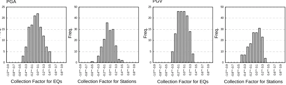
Figure 4 shows the histograms of the collection factor α andβ, and Table 1 shows the standard deviation and correlation coefficient of the collection factors.
Fig.4 Epicenters of the receded Earthquake
Table 1 Standard Deviation and Correlation Coefficient of the Collection Factors
α (Inter-EQs) β (intra-EQs) Total
PGA 0.192 0.251 0.317
Standard
Deviation PGV 0.155 0.263 0.305
Correlation Coefficient 0.873 0.705 0.748
Effects of Magnitude and Focal Distance on Correlation Coefficient
Figure 5 shows the relationship between the magnitude and the correlation coefficient. It is illustrated that correlation coefficient decreases with the increase of magnitude, followed by the regression formula shown below:
95ρ(M)=−0.22M +1. (21)
The similar relationship between the focal distance and correlation coefficient are observed as shown on Fig. 6 with the regression formula shown below:
87ρ(Δ)=−0.00098Δ+0. (22)
Since the greater the magnitude is, the more earthquakes in the far field are contained in the database, it can be concluded that the observation records of the far field make the correlation decrease.
0 5 10 15 20 25 -1 .0 ~-0 .9 -0 .8 ~-0 .7 -0 .6 ~-0 .5 -0 .4 ~-0 .3 -0 .2 ~-0 .1 0. 0
~ 0.
1
0.
2
~ 0.
3
0.
4
~ 0.
5
0.
6
~ 0.
7
0.
8
~ 0.
9
Collection Factor for Stations Collection Factor for EQs
Fr eq. Fr eq. PGA 0 10 20 30 40 50 -1 .0 ~-0 .9 -0 .8 ~-0 .7 -0 .6 ~-0 .5 -0 .4 ~-0 .3 -0 .2 ~-0 .1 0. 0
~ 0.
1
0.
2
~ 0.
3
0.
4
~ 0.
5
0.
6
~ 0.
7
0.
8
~ 0.
9 0 5 10 15 20 25 -1 .0 ~-0 .9 -0 .8 ~-0 .7 -0 .6 ~-0 .5 -0 .4 ~-0 .3 -0 .2 ~-0 .1 0. 0
~ 0.
1
0.
2
~ 0.
3
0.
4
~ 0.
5
0.
6
~ 0.
7
0.
8
~ 0.
9
Collection Factor for Stations Collection Factor for EQs
Fr eq. Fr eq. PGV 0 10 20 30 40 50 -1 .0 ~-0 .9 -0 .8 ~-0 .7 -0 .6 ~-0 .5 -0 .4 ~-0 .3 -0 .2 ~-0 .1 0. 0
~ 0.
1
0.
2
~ 0.
3
0.
4
~ 0.
5
0.
6
~ 0.
7
0.
8
~ 0.
9
Fig.5 Relation between Magnitude and correlation Fig.6 Relation between Distance and correlation
APPLICATION
Condition Setting
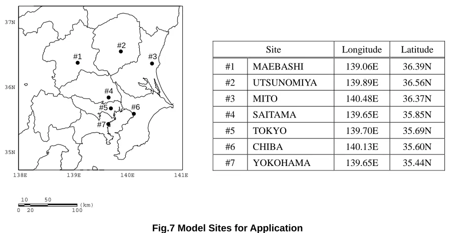
Figure 7 shows the model sites for application. Seismic source zones are given by AIJ[5], in which source zones are categorized into two groups; one corresponds to the large earthquakes modeled as characteristic earthquake, and the other corresponds to background earthquakes modeled by Gutenberg-Richter formula.
Fig.7 Model Sites for Application
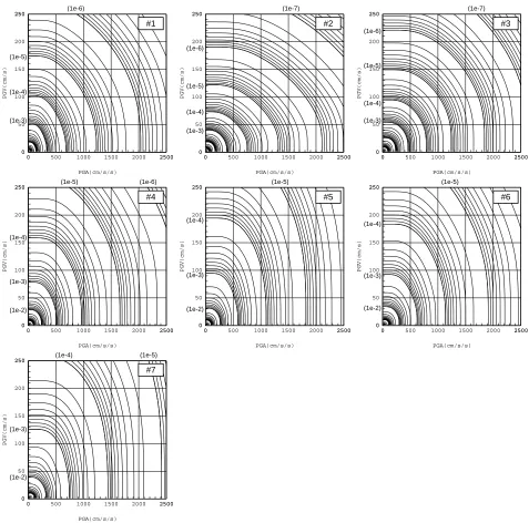
Seismic Hazard Plane for Each Model Site
Figure 8 shows the results of seismic hazard analysis. In this paper, the results are expressed by the contours showing the given probabilities of exceedance. From the figure, it is apparent that the shapes of contours vary with the correlation between PGA and PGV.
By comparing the results for sites in northern Kanto-district with those in southern Kanto-district, it is seen that the ground motion intensities of the former are much smaller than on the latter. It is also observed that the shapes of counters in northern Kanto-district are different from those in southern Kanto-district. The difference in PGV between the former and the latter is greater than one in PGA, since PGV is affected by long period component of ground motions which are generated by inter-plate earthquakes in the southern Kanto-district. It is noted that the famous 1923 Kanto earthquake belong to this types of earthquake.
ρ = -0.2185M + 1.9505
0.0 0.1 0.2 0.3 0.4 0.5 0.6 0.7 0.8 0.9
5.0 5.2 5.4 5.6 5.8 6.0 6.2 6.4 6.6 6.8
地震規模M
相関係
数ρ
ρ = -0.001Δ+ 0.8732
0.0 0.1 0.2 0.3 0.4 0.5 0.6 0.7 0.8 0.9
0 50 100 150 200 250
震源距離Δ(km)
相
関係数
ρ
Magnitude Closest Distance
Corr
el
ation Coef
ficient
Corr
el
ation Coef
ficient
138E 139E 140E 141E
35N 36N 37N
0 10
20 50
100 (km)
#1 Site Longitude Latitude
#1 MAEBASHI 139.06E 36.39N
#2 UTSUNOMIYA 139.89E 36.56N
#3 MITO 140.48E 36.37N
#4 SAITAMA 139.65E 35.85N
#5 TOKYO 139.70E 35.69N
#6 CHIBA 140.13E 35.60N
#7 YOKOHAMA 139.65E 35.44N
#2 #3
#4
#6
#7 #5
Fig.8 Seismic Hazard Plane for Each Model Site
Effect of Correlation Coefficient on Seismic Hazard Plane
Model sites #2, #5 and #7 are selected for the examination of effect of correlation coefficient. Figure 9 shows the results when employing magnitude dependent correlation coefficient as shown on Fig. 5. In evaluating the seismic hazard planes, upper bound and lower bound of correlation coefficient are set to 0.858 and 0.5, respectively. From the comparison of Figs. 8 and 9, it is seen that contours corresponding to low probability are affected by the decrease in correlation coefficient. On the contrary, contours corresponding to high probability are not affected, since seismic hazard with high probability is dominated by the small earthquakes which possess large correlation coefficient between PGA and PGV.
Figure 10 shows the results when employing distance dependent correlation coefficient as shown on Fig. 6. In evaluating the seismic hazard planes, upper bound and lower bound of correlation coefficient are set to 0.846 and 0.6, respectively. From the comparison of Figs. 8 and 10, it is seen that there is small difference in seismic hazard plane of site #2, since there is no large earthquakes that dominates seismic hazard around the site. On the contrary, for sites #5 and #7 close to Kanto earthquake that dominates seismic hazard, the effect of distance dependent correlation coefficient appears.
0 500 1000 1500 2000 2500
0 2500
0 50 100 150 200 250
0 250
PGA(cm/s/s)
PGV(cm/s)
0 500 1000 1500 2000 2500
0 2500
0 50 100 150 200 250
0 250
PGA(cm/s/s)
PGV(cm/s)
0 500 1000 1500 2000 2500
0 2500
0 50 100 150 200 250
0 250
PGA(cm/s/s)
PGV(cm/s)
0 500 1000 1500 2000 2500
0 2500
0 50 100 150 200 250
0 250
PGA(cm/s/s)
PGV(cm/s)
0 500 1000 1500 2000 2500
0 2500
0 50 100 150 200 250
0 250
PGA(cm/s/s)
PGV(cm/s)
0 500 1000 1500 2000 2500
0 2500
0 50 100 150 200 250
0 250
PGA(cm/s/s)
PGV(cm/s)
0 500 1000 1500 2000 2500
0 2500
0 50 100 150 200 250
0 250
PGA(cm/s/s)
PGV(cm/s)
#2 #3
#1
#5 #6
#4
#7 (1e-5)
(1e-5)
(1e-5)
(1e-5) (1e-5) (1e-5)
(1e-5) (1e-4)
(1e-3)
(1e-6) (1e-7) (1e-7)
(1e-6)
(1e-4)
(1e-3)
(1e-6)
(1e-4)
(1e-3)
(1e-6)
(1e-4)
(1e-3)
(1e-2)
(1e-4)
(1e-3)
(1e-2)
(1e-4)
(1e-3)
(1e-2)
(1e-4)
(1e-3)
(1e-2)
Fig.9 Seismic Hazard Plane considering Magnitude-dependent Correlation Coefficient
Fig.10 Seismic Hazard Plane considering Distance-dependent Correlation Coefficient
CONCLUSIONS
In this paper, the seismic hazard analysis using PGA and PGV as ground motion indices is proposed. In constructing the procedure, the correlation coefficient between PGA and PGV is investigated using K-NET and KiK-net databases, followed by the findings that the above-mentioned coefficient is 0.5 and the coefficient may be magnitude dependent as well as distance dependent. By applying the method to some site in Kanto-district, it is also found that the shape of seismic hazard curve is influenced by dominant earthquakes to the site, and by correlation between PGA and PGV.
ACKNOWLEDGEMENT
We give the special thanks to National Research Institute for Earth Science and Disaster Prevention for their acceptance to use K-NET and KiK-net databases for this research.
REFERENCES
1. Sato Y., Fukushima S., Yashiro K.: study on the index of seismic motion for fragility analysis, Summaries of technical papers of Annual Meeting AIJ. B-1, pp. 21-22, 1995.8 (in Japanese)
2. Sakai Y., Yoshioka S., Koketsu K., Kabeyasawa T.: Investigation on indices of representing destructive power of strong ground motions to estimate damage to buildings based on the 1999 Chi-Chi earthquake, Taiwan, Journal of structural and construction engineering, Transaction of AIJ, pp.43-50, 2001.11 (in Japanese)
3. Bazzurro P, Cornell CA.: Vector-valued probabilistic seismic hazard analysis(VPSHA), Proceedings 7th U.S. National Conference on Earthquake Engineering, Boston, MA, 2002.7.
4. Shimomura, T., Takada, T.: Joint pdf of ground motion intensity and duration time based on PSHA, 13th World Conference on Earthquake Engineering, Paper No.1233, 2004.8.
5. AIJ: AIJ recommendations for loads on buildings, 2006.9 (in Japanese)
0 500 1000 1500 2000 2500
0 2500
0 50 100 150 200 250
0 250
PGA(cm/s/s)
PGV(cm/s)
0 500 1000 1500 2000 2500
0 2500
0 50 100 150 200 250
0 250
PGA(cm/s/s)
PGV(cm/s)
0 500 1000 1500 2000 2500
0 2500
0 50 100 150 200 250
0 250
PGA(cm/s/s)
PGV(cm/s)
#5 #7
#2
(1e-7) (1e-5) (1e-6) (1e-4) (1e-5)
(1e-6)
(1e-5)
(1e-4)
(1e-3)
(1e-4)
(1e-3)
(1e-2)
(1e-3)
(1e-2)
0 500 1000 1500 2000 2500
0 2500
0 50 100 150 200 250
0 250
PGA(cm/s/s)
PGV(cm/s)
0 500 1000 1500 2000 2500
0 2500
0 50 100 150 200 250
0 250
PGA(cm/s/s)
PGV(cm/s)
0 500 1000 1500 2000 2500
0 2500
0 50 100 150 200 250
0 250
PGA(cm/s/s)
PGV(cm/s)
#5 #7
#2
(1e-7) (1e-5) (1e-4)
(1e-6)
(1e-5)
(1e-4)
(1e-3)
(1e-4)
(1e-3)
(1e-2)
(1e-3)
(1e-2)