Additive-multiplicative approximation of genotype-environment interaction.

(1)

Additive-Multiplicative Approximation of Genotype-Environment Interaction

A. Gimelfarb

Department of Biology, University of Oregon, Eugene, Oregon 97403 Manuscript received April 21, 1994

Accepted for publication August 20, 1994

the heritability.

G

ENOWE-ENVIRONMENT interactions have

been of interest for a long time, but mainly in the context of animal and plant breeding. More recently this phenomenon started being incorporated into models of evolution in natural populations (VIA and LANDE 1985,1987; GAVRILETS 1986; GILLESPIE and TURELLI 1989;

GAVRILETS and HASTINGS 1994). In spite of the substantial literature on the methods for detecting and estimating genotypeenvironment (GXE) interaction, it is not easy to find a precise definition of it that could be useful for

an evolutionary model of quantitative characters. For example, CALIGARI and MATHER (1975) define GXE interaction as a situation “when, because of their genetic differences, two or more individuals, families or genotypic lines respond differently, or to different extents, to change in the environment.” FALCONER (1983, p. 122)

refers to GXE interaction as a situation in which “a specific difference of environment may have a greater effect on some genotypes than on others, or there may be a change in the order of merit of a series of genotypes when measured under different environments.” Besides not being very precise, such definitions imply that the genotype and environment of an individual can be specified. There are, indeed, instances in which it is possible to specify distinct environments (environmental states), e.g., temperature, density, nutritional level. There are many instances, however, when an identification of an environmental state is very ambiguous, if possible at all. It is definitely not possible in the case of a character influenced by organism’s own internal environments at- tributed “in ignorance of their exact nature to ‘acci- dents’ or ‘errors’ of development” (FALCONER 1983). A

major part of the environmental variation in a quantitative trait is often due to such developmental errors

Genetics 138: 1339-1349 (December, 1994)

ABSTRACT

A model of genotypeenvironment interaction in quantitative traits is considered. The model represents an expansion of the traditional additive (first degree polynomial) approximation of genotypic and environmental effects to a second degree polynomial incorporating a multiplicative term besides the additive terms. An experimental evaluation of the model is suggested and applied to a trait in Drosophila mela- nogaster. The environmental variance of a genotype in the model is shown to be a function of the genotypic value: it is a convex parabola. The broad sense heritability in a population depends not only on the genotypic and environmental variances, but also on the position of the genotypic mean in the population relative to the minimum of the parabola. It is demonstrated, using the model, that G X E interaction may cause a substantial non-linearity in offspring-parent regression and a reversed response to directional selection. It is also shown that directional selection may be accompanied by an increase in

rather than environments external to the organism (FALCONER 1983), and, consequently, “internal” environments may play an important role in the evolution of quantitative traits.

The traditional and most widely used in quantitative genetics approach to dealing with the genotype environment interaction is based on a partitioning,

v,

=

v,

+

v,

+

v,,

( 1 )

of the phenotypic variance of a trait, V,, into genotypic,

V,, environmental, V,, and interaction, V,,, components. Underlying such variance partitioning is the decomposition of the phenotype of an individual into the “main effects” of the genotype and environment, and their “interaction,”

X = G + E + I , . (2)

(2)

1340 A.

out by VIA and IANDE (1985) about the model ( l ) , “obtained within its frame estimates of genotypeenvironment interaction cannot be incorporated in any current theory of evolution.”

ADDITIVE-MULTIPLICATIVE MODEL OF GXE INTERACTION

Almost any work dealing with the dynamics of quantitative traits uses the following model to express the notion that the phenotype of an individual is determined by its genotype and by the environment to which it is exposed:

X = x + e, (3)

where x and e are the contributions to the phenotype by the genotype and environment, respectively. This model has been around for such a long time that it is sometimes regarded as representing a biological mechanism of character development. Recalling, however, the enor- mous complexity of biochemical pathways for even very simple phenotypes (with different genes and environments acting at different developmental stages), it should be obvious that the only thing that can be stated with a certainty about mechanisms of character development is that, whatever they are, they result in a mapping,

X = F{genotype, environment}, (4)

of genotypes and environments onto the phenotype, and that this mapping is almost certainly very complex. One way to get around this problem is to postulate that a numeric value (contribution) can be assigned to a genotype as well as to an environment, and to seek an approximation of mapping (4) by a simple mathematical function of the genotypic and environmental contributions. The additive model (3) is the simplest such approximation by a first degree polynomial in two variables, rather than a description of a specific biological mechanism. The adequacy of the additive approximation for a particular trait can be used to define the presence or absence of GXE interaction in this trait. If the approximation is sufficiently good, we can say that the genotype and environment do not interact. If, on the other hand, the additive approximation is not adequate, this means that there is GXE interaction, and an approximation by some other mathematical function is needed. A simplest extension of model (3) approximat- ing GXE interactions is a second degree polynomial in two variables which incorporates a multiplicative term in addition to the additive terms:

X = = x + e + Dxe.

(5)

Parameter D in (5) can take any value between minus and plus infinity. It characterizes the strength of GXE interaction: there is no interaction if D = 0,

whereas larger values of D indicate more multiplicative

interaction. If rewritten as

X = x

+

ye, ( y = 1

+

D X ) , (6)

expression (5) becomes a special case of the more gen- eral model by GAWLETS and HASTINGS (1994) whose parameter y is determined by the whole multilocus genotype of the individual rather than by its genotypic contribution, as in the above model. Regarding phenotypes as functions of environmental contributions, model (5) represents a special case of the model of “linear reaction norms” (DE JONC 1990a).

The idea of environment contributing multiplica- tively to the phenotype is not new. The first experimental evidence for environmental multiplicativity comes from an investigation by FISHER and MACKENZIE (1923) of the response by potato varieties to different environments. They concluded that “the yields of different varieties under different manurial treatments are better fitted by a product formula than by a sum formula”

[quoted by FREEMAN (1973)l. A purely multiplicative model (without additive terms) was considered by MATHER (1975) who discussed instances in which such a model describes the action of genes and environment better than the additive model does. GIMELFARB (1986)

has studied the behavior of the purely multiplicative model under directional selection. GAWLETS (1986) used a model similar to (5) to investigate the effect of

GXE interaction on the maintenance ofvariation under stabilizing selection. He suggested an interpretation of the terms in the model as the environment-independent effect of genes, the effect of a change in the composition of active genes, and the effect of a change in the activity of genes.

We shall assume that the genotypic, x, and environmental, e, contributions in (5) are distributed indepen- dently of each other with the mean and variance of x denoted as m, and u,, and with the mean and variance of e denoted as m, and u,. It is not difficult to see that in the additive-multiplicative model (5), the phenotypic mean, M , and the phenotypic variance, V, are as

M = m,

+

m,

+

Dm,m,,

(7)

V = u,(l

+

DmJ2

+

u,(l

+

Dm,)’

+

D2u,ue. (8)

An environment can be classified as either “micro” or “macro” depending on whether the environmental differences are between individuals in the same population or in different populations. Organism’s internal “acci- dents” or “errors” of development (FALCONER 1983) r e p resent an example of micro environment, although con- ditions external to an organism, such as temperature or nutritional level, may also be microenvironmental. On the other hand, differences between animal or plant farms, as well as between natural habitats are examples of macro environment. Both micro and macro environments can be handled within the framework of model

(3)

population 111

FIGURE 1 .-Parabola describing the environmental variance of a genotype as a function of the genotypic contribution (dashed curves represent populations with different distributions of the genotypic contributions).

GENOTYPIC CONTRIBUTION

micro environments, except for the last section dealing with GXE interaction and genetic correlation.

The mean value of microenvironmental contributions can be set to zero without loss of generality (by linear rescaling of the phenotype). Consequently,

(7)

and (8) can be rewritten as

M = m,, (9)

V = v,

+

v,(l

+

DmJ2

+

D2v,ve. (10)

Thus, in the additive-multiplicative micro environment, the mean of a trait in a population can be assumed equal to the mean genotypic contribution. It is also seen from

(10) that, unless D = 0, i.e., the environmental contribution is strictly additive, the variance of the trait is determined not only by the variances of the genotypic and environmental contributions but also by the mean genotypic contribution, or by the mean of the trait in the population (given (9) )

.

ENVIRONMENTAL VARIANCE OF A GENOTYPE Given a group of genotypically identical individuals, the phenotypic variance of a trait among them can be regarded as the environmental variance of their genotype. If environment is strictly additive, this variance is determined only by the variance of environmental contributions and, hence, it is the same for any genotype. This is not true, however, if environment is not additive. Let a group of individuals with a common genotype g whose contribution to a character is x be exposed to additive-multiplicative environment. Given the genotypic identity of the individuals, the variance of the genotypic contributions in the group is zero, i.e., v X = 0,

and the mean in the group is simply the genotypic contribution to the character, i.e., m, = x. Substituting these values into ( l o ) , we obtain the environmental variance of the genotype g as

V ( g ) = v,(l

+

D X ) ~ . ( 1 1 )

It is seen that V( g ) is determined not only by the variance of environmental contributions but also by the genotype. As a function of the genotypic contribution, x, it is a convex parabola with the minimum at the point

p = - 1 / D . (12)

An example of such parabola is represented by the solid curve in Figure 1. Dashed curves in the same figure cor- respond to populations with different distributions of

the genotypic contributions. Depending on the position of the mean of the genotypic contributions relative to the minimum point

(12),

the environmental variance of a genotype in the population can be either a decreasing function of the genotypic contributions (population I) or an increasing function (population 111) or a non- monotone function (population 11).

GILLESPIE and TURELLI (1989) proposed a model of genotype-environment interaction based on the assumption of higher developmental homeostasis of multilocus heterozygotes. An important property of their model is that the environmental variance of a genotype is a decreasing function of the number of heterozygous loci in the genotype. If contributions by the loci to the trait are additive, genotypes with intermediate contributions will have on the average a higher proportion of heterozygous loci than those with more extreme contributions. Consequently, the environmental variance will be lower for genotypes with intermediate contributions than for genotypes with more extreme ones. As a function of the genotypic contribution, the environmental variance will resemble a convex parabola. It a p pears, therefore, that the model of GXE interaction by GILLESPIE and TURELLI (1989) can be approximated by the additive-multiplicative model (5).

(4)

10

9 8

7

5,

R

I

5

4 3

7

I I I I I I I I

28 32 38 40 44 48 52 58 8 0 MEAN

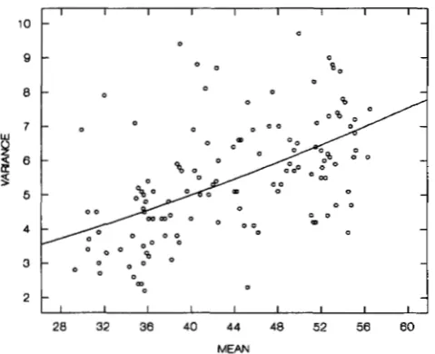
FIGURE 2.-The relationship between the mean and the vari- ance of abdominal bristles in isogenic lines of D. melanogaster (each point represents an isogenic line).

least squares fit of (1 1) to the data yields a parabola (the solid curve in Figure 2) with the following parameters:

D = 0.021, v, = 1.475. (13)

The minimum point of the parabola, p = -47.6. Since the number of bristles cannot be negative, the negative value of p implies that for the abdominal bristles in D. melanoguster the minimum point is located always outside and to the left of the distributional range of the genotypic contributions (as for population I11 in Figure l ) , and, hence, the environmental variance of a genotype is always an increasing function of the genotypic contribution.

For any parameter D # 0 , the model (5) can be rewritten as

X + 1/D = (x

+

1/D)(1

+

De). (14)

This means that the additive-multiplicative model with a non-zero parameter D is equivalent to the purely multiplicative model with phenotypes and genotypic contributions measured from the minimum point, p =

-

1/D, of the parabola (1 1)

,

and with the distribution of environmental contributions having the mean equal to 1 and the variance equal to v&‘.

VARIANCE PARTITIONING AND HERITABILITY

The phenotypic value of any quantitative trait can be decomposed according to the statistical model (2) into the main genotypic and environmental effects and their interaction. It is shown in APPENDIX A that under the additive-multiplicative model,

G = x, (154

E = e(1

+

Dm,), (15b)

ZGE

= De(x - m,). (15c)

Expressions nents of the

for the corresponding variance compo- total phenotypic variance follow as

v,

= v,, (16a)

V’ = v,(l

+

Dm,)‘, (16b)

v,

= v , v p , (16c)

The genotypic effect, G, of an individual is often called its “genotypic value.” Hence, in the additive- multiplicative model of environment, the genotypic value is the same as the genotypic contribution, x, and the genotypic component of variance is the variance of the genotypic contributions. Equations 16 lead to the following expression for the broad sense heritability of a trait under additive-multiplicative environment:

H z = v,/[v,

+

v,(l

+

DmJ2

+

v , v p ] . (17)

It is seen that in the presence of GXE interaction (D #

0), the heritability is determined not only by the variances of the genotypic and environmental contributions but also by the mean of the genotypic contributions, or, given (9), by the mean of the trait. Consequently, a shift in the mean may cause the heritability to change.

In the laboratory population of D. melanoguster from which the genetically homogeneous lines discussed earlier had been extracted, the mean and the variance of the abdominal bristles among females were, respectively, M = 44.2 and V = 14.4. Making use of (9) and substituting these values, together with estimates (13) of D and v,, into (10) yields the genotypic variance v, = 8.81 leading to the prediction of H z = 0.61 for the broad sense heritability. Unfortunately, no direct estimate of the heritability in the laboratory population from which the lines were extracted is available, and it is not possible, therefore, to compare the predicted heritabilitywith the actual value of the heritability in the laboratory population. We may, however, compare it to the estimates of the broad sense heritability for abdominal bristles re- ported in the literature. For example, FALCONER (1981, Table 8.2) presents data by CLAY~ON et ul. (1957) yield- ing an estimate of H z that happens to be exactly identical to the predicted above value of 0.61 (but see FAL-

CONER’S Example 8.6 in which H z = 0.55 for a different strain of flies).

Expression (17) for the heritability can be rewritten as

H z = 1/[1

+

vp’(1

+

&)I,

(18)

where parameter

(5)

Interaction

I I I I I I I

A

H2

-

0.25

-

4 - 5 0

" -

d

-

20

d - 10

" _ -

-3 -2 - 1 0 1 2 3

d = 10

-3

3

2

1

0

- 1

-2

-3

I I I I I I 1

B

Hz

-

0.25

- d = 4.0

" _

d = 2.0 d = 1.0

d = 0.0

" "

. . .

I I I I I I L

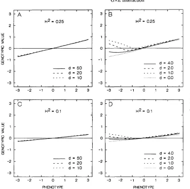
-3 -2 - 1 0 1 2 3 FIGURE 3.-The regression of

the genotypic value -on pheno-

I r I I I I type for different values of the

3

- D

-

_{broad heritability,}

p ,

and param-

Hz = 0.1 eter d.

d

-

2.0 d = 1.0

d = 0.0 -2

-3

-3 -2 - 1 0 1 2 3 -3 -2

PHENOTYPE

additive-multiplicative environment with given parameters u, and D, the broad heritability is completely determined by parameter d. Since the heritability is a decreasing function of d, it is maximized in a population in which d = 0, i.e., the genotypic (phenotypic) mean is exactly at the minimum point of parabola (1 1). The maximum value of the heritability that can ever be main- tained in any population by a trait with given parameters ue and D is obtained by substituting d = 0 into (18):

H2,,= 1/(1

+

u p ) . (20)

GXE INTERACTION AND OFFSPRINGPARENT REGRESSION

The regression of the offspring's phenotype, Z, on the parental phenotype, X , can be expressed as

E[ZI

Xl

= J E [ z l x]flxl

X)

dx, (21)

(given that the mean of environmental contributions to the character is zero). E [ z I x] in here is the regression of the offspring's genotypic contribution (genotypic value) on the parental genotypic contribution (genotypic value), and

P(

x I X ) is the probability that the genotypic contribution of a parent with phenotype X is x.

- 1 0 1 2 3 PHENOTYPE

If genes controlling a quantitative trait act strictly additively, the Mendelian segregation implies E [ z I x] = %x, and consequently,

E[ZI = $[x1 x], (22)

i e . , the offspring-parent phenotypic regression for a character with additive gene action is equal to one half of the regression of genotypic values on phenotypes among parents.

Based on a mathematical result of LINDLEY (1947), NISHIDA and A B E (1974) demonstrated that the regression E [ x I

x]

(and, hence, the offspring-parent regression) can be nonlinear in the absence of GXE in-

teraction, if the distributions of the genotypic and environmental contributions are not normal. On the other hand, GXE interaction itself can render this regression nonlinear, even if both genotypic and environmental contributions are normal.

(6)

1344

were assumed to be normal. The genotypic values (ver- tical axis) and phenotypes (horizontal axis) are measured as the deviations from the mean in the genotypic standard deviations, i. e., as ( x - m ) /a, and ( X - M ) / u x , respectively. In the case of strictly additive environment, their ratio is equal to the broad heritability, H z .

Computational details are discussed in APPENDIX B.

Regressions were computed for different values of parameter d , the standardized distance between the genotypic mean in the population and the minimum point of the parabola (1 1). Regressions for only positive values of d are shown. The regression for a negative value of d can be obtained by a 180” rotation of the graph for the corresponding positive d .

The first thing to notice in Figure 3 is that the regressions can be quite different even for the same heritability, depending on the position of the mean in a population relative to the minimum point of parabola

(11). If d

>

4 (Figure 3, A and C ) , the regressions are practically linear (at least for the phenotypes within the 2 3 standard deviations interval). On the other hand, the offspring-parent regressions are nonlinear, if d 5 4 (Fig- ure 3, B and D ) . The regression can even be non- monotone in the latter case.

It should be recalled that the offspring-parent regressions, E [ Z I x], will be similar to the regressions E [ x I

x]

shown in Figure 3, if the action of genes controlling a quantitative character is additive. If, on the other hand, the genes act non-additively, the offspring- parent regressions, while almost certainly remaining nonlinear for d 5 4, may have shapes differing from those in Figure 3.

GXE INTERACTION AND SELECTION

If a quantitative trait, X , is under selection with a phenotypic function

w(

X ) , the fitness of an individual with genotypic contribution x and environmental contribution e is as

w ( x , e) = W x

+

e

+

Dxe), (23)

given the additive-multiplicative environment (5). The genotypic fitness function, w ( x) L e . , the average fitness of an individual with the genotypic contribution x is

4 x 1 =

II

w ( x , e)q(e) de, (24)

where q( e ) is the distribution of the environmental contributions which is assumed to have zero mean and variance u,. The familiar expression determines the distribution of the genotypic contributions after selection,

p*

(x), for a given distribution of the genotypic contributions before selection,

p (

x):

p ( 4*

= p ( x ) w ( x ) / w , (25)

W= l p ( x ) w ( x ) dx. (26)

In this study, we shall concentrate on the distribution of the genotypic contributions among selected parents. The distribution of the genotypic contributions, and, hence, the phenotypic distribution among the offspring of these parents will be determined by the distribution

p*

( x ) as well as by the mechanisms of hereditary trans- mission and the action of genes controlling the trait. The distribution of the genotypic contributions, $I( x), as well as the distribution of the environmental contributions,

q(

e ) , will be assumed normal.

Directional selection: We shall refer to directional selection as upward or downward, depending on whether individuals with higher or lower phenotypes are favored by selection. Since the broad heritability of a trait under additive-multiplicative environment is a decreasing function of the distance between the genotypic mean and the minimum point of parabola (1 1)

,

directional selection may increase the heritability, if the mean is moved by selection closer to the minimum point. Thus, in a population with the mean to the left of the minimum point (population I in Figure 1) under upward selection, or with the mean to the right of the minimum point (population 111 in Figure 1 ) under downward selection, the broad heritability may increase as a result of selection, even if the genotypic variance among offspring is the same as among their parents (an assump tion often made in quantitative genetics).

Considering expression

(17) for the heritability no-

tice that if populations with different mean genotypic contributions have similar heritabilities, it implies that the populations have different variances of the genotypic contributions. Hence, it is not possible for the genotypic component of variance (16a) and for the heritability to remain both unchanged, if the mean changes. This means that models of directional selection assuming that both the genotypic variance and the heritability remain constant in the process of selection are suspect, if they are applied to traits with GXE interaction.

Exponential selection: In the case of directional selection with the phenotypic fitness function W ( X ) = exp ( S X )

,

the genotypic fitness function is also exponential, if environment is purely additive. This is not true, however, if there is GXE interaction. Given a normal distribution of environmental contributions in the additive-multiplicative model (5), the genotypic fitness function implied by exponential selection on the phenotype can be shown to be as

w ( x ) = exp[Q(x - 8)‘1, (27)

8 = -(1

+

SUeD)/(SV,D‘), (28)

Q = S ‘ U J Y . (29)

where

(7)

distribution of genotypic values before selection is normal, and the following constraint on selection holds:

9 <

1/(v,vP2), (30)

the distribution of the genotypic values after selection,

p*

(x),

can be shown to be also normal with the mean and the variance:

mz = [m,

+

(S

+

vJS)v,]/(l - v,zleD2P), (31)

vz = vJ(1 - v , v e b 9 ) . (32)

Equation 31 implies the following expression for the genotypic selection differential, i. e., the difference between the means of the genotypic values after and before selection:

u,S[1

+

u,D2S(m, - p)]

mr - m, =

1

-

V ~ V , D ~ S * 9 (33)

where p is the minimum point of parabola (1 1 ) . It is seen that, depending on the position of the mean relative to p, the genotypic selection differential can be negative under upward phenotypic selection and positive under downward phenotypic selection. The possi- bility thus exists for a reversed response to directional selection in exponential form by a trait with GXE interaction. A necessary condition for this is that m,

<

p, if selection is upward (S > O ) , and m,

>

p, if selection is downward ( S < 0 ) . This means that under upward selection the environmental variance must be a decreasing function of the genotypic value (population I in Figure l ) , whereas it must be an increasing function (population I11 in Figure 1) under downward selection. These conclusions are in agreement with the logic of the reversed response to selection suggested by HALDANE

(1966, pp. 176-179). However, exponential selection must be extremely strong in order for a reversed response to actually occur. For example, calculations show that a reversed response in a population with the heritability H z = 0.1 is possible only if the strength of selection is such that there is at least a twofold difference between the fitnesses of individuals whose phenotypes are only one standard deviation apart. Selection must be even stronger for higher heritabilities.

Threshold selection: Consider selection such that individuals with the phenotypes above (upward selection) or below (downward selection) a threshold value

T are selected as parents. Utilizing the fact that the additive-multiplicative model (5) can be transformed into a purely multiplicative model (14), it follows from results of GIMELFARB (1986) for the latter model that the genotypic fitness function for upward selection is as

10

0 8

0.6

0 4

0.2

z

-

0.0

-

1.0

-

2.0

-

3.0

0 0 I J

-4 -3 -2 -1 0 1 2 3 4

GENOTYPIC VALUE

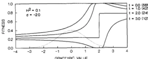
FIGURE 4.-Genotypic fitness functions corresponding to threshold phenotypic selection with different threshold val-

ues, t (corresponding percent of selected individuals is indicated in parentheses).

where +( z ) denotes the cumulative distribution func- tion of a standardized normal distribution (the integral from --CO to z). The genotypic fitness function for downward selection is similar, except that expressions

(34a) and (34b) are for x

<

0 and

x

>

0 , respectively. An example of genotypic fitness functions for upward selection with different threshold values in a population with H 2 = 0.1 is presented in Figure 4. The genotypic values as well as threshold values, t, are measured as distances in genotypic standard deviations from the population mean, i.e., as

(x

- m , ) / u , and

( T - m,)/u,, respectively. The percentage of individuals selected under selection with a particular threshold is indicated in parentheses next to the

threshold value. The dashed curve shows the distribution of the genotypic values in the population. It is assumed that d = -2, i.e., the genotypic mean is located two genotypic standard deviations to the left of the minimum point of parabola ( l l ) , ie., the popu- lation is similar to population I in Figure 1.

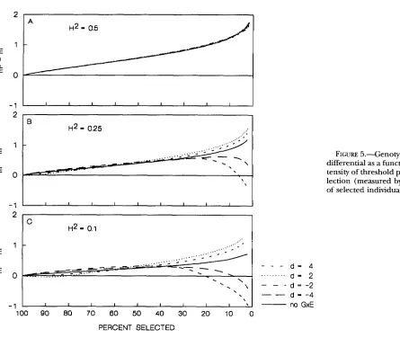
It is not possible to obtain an analytical expression for the mean genotypic value after selection, mz, for the fitness function (34), and numeric calculations have to be employed. Figure 5 shows the genotypic selection differential, m: - m,, as a function of the selection intensity under upward threshold selection. Different values of H z and parameter d are considered. The no- tation “no GXE” refers to curves obtained under the assumption that genotypic and environmental contributions are purely additive. Intensity of selection (meas ured by the percent of selected individuals) increases from the left to the right side of a graph.

Curves in Figure 5A are practically indistinguishable from each other. This means that GXE interaction has no effect on the response to threshold selection in a population with H z = 0.5, irrespective of the position of the mean relative to the minimum point of parabola

(8)

2

A

H2

-

0.5

E 1 -

I

.

_E

0

- 1

2

I I I I I I I I I

B

H2

-

0.25

..' ,

,.. ,

1 -

E

I

E -0 .. . . \

,

-1

2

- I I I I I I I I I

C

H2

-

0.1

1 - ...' ,

E ,_..' ...'

.

I

E

" _

d - 4

d - 2

'.

\ " * d " 2

,

-

no GxE

I I I I I I I I I

d

-

-4

. . .

.

\

.

"

,

- 1

1 0 0 90 80 70 60 50 40 30 20 PERCENT SELECTED

although not necessarily unrealistically strong (e.g., 20% or less selected, H z = 0.1, and d =

-2).

Notice that a reversed response is possible not only under strong selection, but under weak selection as well (the dashed curve in Figure 5c in the interval with 80% or more selected). Given that selection is weak, the genotypic selection differential is, of course, quite small, but it is clearly negative. The cause of this is the nonlinearity in the regression of the phenotype on the genotypic value discussed earlier. This finding confirms a conclusion by GIMELFARB and WILLIS (1994) that a nonlinearity in the offspring-parent regression can have a profound effect on the response to selection not only if selection is very strong, but also if it is weak.

Stabilizing (quadratic) selection: If a quantitative character is under stabilizing selection with a quadratic phenotypic fitness function,

W ( x ) = 1 - S ( X -

0)2,

(35)

given that there is additive-multiplicative GXE interaction and that the distribution of genotypic contributions is normal, the genotypic fitness function can be shown to be as

w(x) = 1 - Q(x - 0 ) 2 , (36)

10 0

FIGURE 5.-Genotypic selection differential as a function of the intensity of threshold phenotypic selection (measured by the percent of selected individuals).

where

0 = 0/(1

+

u p ' ) . (37)

Q =

S(1

+

u,D')'/[~

+

v,D'(1 - S(O - p)')]. (38)

Thus, the genotypic selection is also quadratic. This means that the genotypic variance of a character under additive-multiplicative environment is always decreased by quadratic stabilizing selection. Notice, however, that the optimum genotypic value, 0, is not the same as the optimum phenotypic value, 0. Hence, the mean of a quantitative character in a population at equilibrium under quadratic stabilizing selection may not coincide with the optimum phenotype, as a result of GXE interaction.

GXE INTERACTION AND GENETIC CORRELATION

This is the only section in the paper in which macro environments ( e . g . , different farms or natural habitats) rather than micro environments are considered. FAL- CONER (1952) proposed to treat the phenotypes expressed by identical genotypes in different macro environments as separate traits. Based on this, VIA and LANDE

(9)

in natural populations. The coefficient of genetic correlation between such “traits” is regarded as an indicator of GXE interaction. It is asserted that the genotype and environment do not interact if the correlation is perfect. If, on the other hand, the correlation is less than perfect, it is taken to be an indication of GXE interaction.

It is important to realize, however, that a perfect genetic correlation between phenotypes expressed by the same genotype in different environments does not necessarily mean the absence of GXE interactions. Using a “reaction norm”mode1, DE JONC (1990b) has shown that the genetic correlation can be equal to

+

1, even if the component of variance due to GXE interaction is not zero. Additive-multiplicative model

( 5 )

provides an- other proof of this. Consider, for example, two distinct macro environments, and let phenotypes in both environments be determined by the additive- multiplicative model with parameter D . Assume that the mean and variance of the environmental contributions are m: and v: in one environment, and my and v:in the other environment. If

x

is the contribution by a genotype to the character, equation (A8a) in APPENDIX A implies that the genotypic values, G’ and G“, of the genotype in the two environments are

G’ = x(1

+

Dm:) - Dmlm:, (394

G = x(1

+

Dm3 - D r n ~ r n ~ . (39b)

It is seen that the two genotypic values are linearly re- lated. Hence, they are perfectly correlated for any value of parameter D. Hence, the genetic correlation between two “traits” can be perfect even in the presence of a strong GXE interaction.

CONCLUSIONS

The environmental variance of a genotype can be a function of the genotypic value (convex parabola in the additive-multiplicative model).

The broad sense heritability in a population can be determined not only by the genotypic and environmental components of variance, but also by the mean of the character in the population. Consequently, a shift in the mean due to selection or other evolutionary forces may cause a change in the heritability, even if the components of variance remain unchanged.

The regression of the genotypic value on the phenotype and, hence, the offspring-parent regression can be non-linear.

GXE interaction may have a very profound effect on the response by the mean of a quantitative character to directional selection. It may even cause a reversed response to threshold selection, not only if selection is strong, but also if it is very weak.

The broad sense heritability may either decrease or increase under directional selection, depending (in the

additive-multiplicative model) on the position of the mean genotypic value relative to the minimum point of the parabola describing the environmental variance of a g e n e type. It is not possible for both the heritability and the genotypic component of variance to remain unchanged, if the mean of the character is changed by selection.

GXE interaction (in the additive-multiplicative model) has little effect on the response by the variance of a quantitative character to stabilizing selection. The mean of a trait in a population at equilibrium may not coincide, however, with the optimum phenotype.

If the mean phenotypes expressed by the same genotype in two different macro environments are treated as separate traits, the genetic correlation between them can be perfect, even in the presence of GXE interaction.

The data on the isogenic lines of D. melanogaster were collected years ago at the Agrophysical Institute in Leningrad by GALINA KOVAI.

and GALINA EPELMAN to whom I wish to express my most profound gratitude. This work was supported by U S . Public Health Service grant GM27120.

LITERATURE CITED

CALIGARI, P. D. S., and K. MATHER, 1975 Genotypeenvironment interaction. 111. Interactions in Drosophila melanogaster. Proc. R. SOC. Lond. B 191: 387-411.

CLAYTON, G.A.,J.A. Moms andA. ROBERTSON, 1957 An experimental check on quantitative genetical theory. I. Short-term responses to selection. J. Genet. 5 5 131-151.

DE JONG, G., 1990a Quantitative genetics of reaction norms. J. Evol. Biol. 3: 447-468.

DE JONG, G., 1990h Genotype-byenvironment interaction and genetic covariance between environments: multilocus genetics. Genetics 81: 171-177.

FALCONER, D. S., 1952 The problem of environment and selection.

Am. Nat. 86: 293-298.

FALCONER, D. S., 1983 Introduction to Quantitative Genetics, Ed. 2. Longman, New York.

FISHER, R. A., and W. A. MACKENZIE, 1923 Studies in crop variation. 11.

The manurial response of different potato varieties. J. Agric. Sci.

13: 311-320.

FREEMAN, G. H., 1973 Statistical methodsfor the analysis of genotypeenvironment interactions. Heredity 31: 339-354.

GAVRILETS, S., 1986 An approach to modeling the evolution of populations with consideration of genotypeenvironment interaction (translation from Russian). Sov. Genet. 22: 28-36.

GAVRILETS, S., and A. HASTINCS, 1994 A quantitative genetic model for

selection on developmental noise. Evolution (in press). GILLESPIE, J. H., and M. TURELLI, 1989 Genotypeenvironment inter-

actions and the maintenance of polygenic variation. Genetics 121:

GIMELFARB, A., 1986 Multiplicative genotypeenvironment interaction as a cause of reversed response to directional selection. Genetics 114: 335-343.

GIMELFARB, A., and J. H. WILLIS, 1994 Linearity versus nonlinearity in offspring-parent regression: experimental study of Drosophila melanogaster. Genetics 38: 343-352.

HALDANE, J. B. S., 1966 The Causes of Evolution (Dornell paper- backs). Cornell University Press, Ithaca, New York.

LINDLEY, D. V., 1947 Regression lines and the linear functional relationship. J. R. Statist. SOC. Suppl. 9: 218-244.

MATHER, K., 1975 Genotype X environment interactions. 11. Some genetical considerations. Heredity 35: 31-53.

NISHIDA, A., and T. A B E , 1974 The distribution of genetic and environmental effects and the linearity of heritability. Can. J. Genet. Cytol. 16: 3-10.

(10)

1348

VIA, S., and R LANDE, 1987 Evolution of genetic variability in a spatially heterogeneous environment: effects of genotpe- environment interaction. Genet. Res. 49: 147-156.

Communicating editor: M. SLATKIN

APPENDIX A

In the statistical decomposition model

(2),

the main genotypic effect, G, is determined strictly by the genotype, whereas the main environmental effect, E, is determined strictly by environment. The sum of G and

E

gives the least squares fit to the phenotypes in the population. Hence, in order to obtain the main effects for a character with phenotypic values determined by the additive-multiplicative model ( 5 ) , it is necessary to find functions G( x) and E ( e ) such that they deliver the minimum of the integral

111

[ x

+

e

+

Dxe - G(x) - E(e)]*p(x)q(e) dx de (Al) under the constraints

~ G ( x ) P ( x ) d x = m,, (-424

I.(e)de) de = me, (A2b)

e

where p ( x ) and q ( e ) are the distributions of the genotypic and environmental contributions, respectively. Let us consider the functions G( x) and E( e ) in a linear form:

G(x) = a x

+

p,

(A34

@e) = ye

+

6. (A3b)

It follows from ( M a ) and ( M b ) that

J3 = m, - am,, 6444

6 = me - ym,. (-44b)

Substituting (A3) and (A4) into (Al) and differentiating (Al) with respect to a and y, we obtain the following normal equations:

JJ(x - m x ) [ ( 1 - a ) ( x - mx)

+

(1

-

r>(e - me) (A54

+

Dxe]p(x)q(e) d x de = 0 ,

[ [ ( e - m , ) [ ( 1 - a>(x - m,)

+

(1 - ?>(e - me> (fib)

+

Dxe]p(x)q(e) dx de = 0 ,

or, after integrations,

v,(l - CY

+

Dm,) = 0 , (A64

v,(l - y

+

Dm,) = 0. (A6b)

The latter equations yield

CY = 1

+

Dm,, (A74

y = 1

-+

Dm,. A7b)

Consequently, the main genotypic and environmental effects are:

G = x(1

+

Dm,) - Dm,m,, ( A 8 4

E = e(1

+

Dm,) - Dm,me. (A8b)

The interaction effect is then obtained by subtracting the sum of G and E from the right side of expression

( 5 )

:

IGE

= D[mxm,

+

(x - m,)(e - m , ) ] . (A9)

Since for a microenvironment the mean of the environmental contribution can be set to zero,

G = x, (AlOa)

E =

41 +

Dm,), (AlOb)

IGE

= DE(X - m,) (AlOc)

in a such environment. The expressions (16) for the variance components follow from the above equations.

APPENDIX B

Let P( x , X ) be the joint distribution of genotypic contributions and phenotypes. The regression of x on Xcan be computed as

E[xl

Xl=

l q x , X ) d x / S x 1 (BW

= J.p(X)flXlX)

dx/

Jp(x)SxI

X

4

dx, (Bib)

where

p (

x) and P( X) are the distributions of the genotypic contributions and phenotypes, respectively, and

P( X I x) is the distribution of phenotypes among individuals with the genotypic contribution x. If q( e ) is the distribution of environmental contributions in the additive-multiplicative model ( 5 ) , the following expression for P( XI x) is straightforward:

The regression E [ x I x] can be obtained by substituting this into (Blb) and computing numerically the integrals for given distributions

p (

x) and q ( e ) . Assuming that these distributions are normal, the four parameters have to be specified in order to carry out the calculations for micro environments: the mean and variance of x, the variance of e, and the value of D .

Transforming phenotypes as X' = ( X - M ) / a x , model ( 5 ) becomes

(11)

where, given that M = m,,

x' = (x - m , ) / a , , (B4)

e' =

41 +

D m , ) / u x , (B5)

D' = Da,/(l

+

Dm,). (B6)

It follows from (B4) that

mi = 0, v i = 1. (B7)

Using parameters p in (12) and d in (19), Equation B6 can be rewritten as

D l = - - a x 1

"

m x - p d '

Consequently, p' = -l/D' = d, and

for the transformed variables. The heritability for the transformed model (B3) is the same as for non- transformed model (5), since both the phenotype and the genotypic contribution are transformed similarly. Hence, given (B7) and (B8a,b), expression (18) for the heritability can be rewritten as

H 2 = 1/[1

+

vi(D')2(1

+

(B94

= 1/[1

+

v:

+

v:/d2]. (B9b)

The mean and variance of e' are obtained from (B5) and (B9b) as

Given (B7), (B9) and (BlO), only two parameters,

Additive-multiplicative approximation of genotype-environment interaction.