R E S E A R C H
Open Access
ENCP: a new Energy-efficient Nonlinear
Coverage Control Protocol in mobile sensor
networks
Zeyu Sun
1,2*, Guozeng Zhao
1and Xiaofei Xing
3Abstract
The node deployment in mobile sensor networks (MSNs) is mostly performed in a random method. However, a large number of redundant nodes may exist due to the randomness. As a result, severe data congestion may be caused and the quality of coverage (QoC) is undermined. In order to solve this QoC problem, we propose an Energy-efficient Nonlinear Coverage Control Protocol (ENCP). This protocol utilizes the normal distribution to calculate the minimal number of sensors which is required to guarantee coverage over the monitoring area. We also balance the node energy consumption and achieve the collaborative scheduling among all the sensor nodes. Meanwhile, when a certain QoC is guaranteed, we present the calculation model for the normal distribution of the sensing ranges and the proportional relationship between different parameters in the QoC function. Finally, simulation results show that the ENCP could not only improve the network QoC and network coverage rate but also effectively control the energy exhaustion at the nodes. Therefore, the network lifetime can be effectively prolonged.
Keywords:Mobile sensor network, Nonlinear coverage, Quality of coverage, Networks coverage rate, Network lifetime
1 Introduction
Mobile sensor networks (MSNs) are composed of tens of thousand sensor nodes whose processing ability, com-munication bandwidth, and energy are quite limited. Usually, the high-density node deployment strategy is employed to improve the network performance [1]. The node density can be as high as 200 nodes/m2. However, a series of problems are brought about in terms of scal-ability, information redundancy, wireless channel inter-ference, and energy wastes. Since the sensors are mostly battery-powered, it is often impractical to replace the batteries due to the limits of the application environ-ment. However, the network is expected to work over a long period of time without further energy supply, which makes the energy management a key problem for the study of sensor networks.
The node scheduling enables the switching between dif-ferent states of the nodes, utilizing the node redundancy and the heuristic algorithms [2, 3]. The aim of the node scheduling is to save the node energy and prolong the net-work lifetime with the desired QoC by shutting down the nodes in turn. Currently, most coverage control algorithms obtain the coverage information according to the location information of the nodes [4–6]. However, the acquisition of location information relies on external infrastructures such as the GPS and directional antennas, which greatly in-creases the hardware cost and energy consumption for the nodes. Meanwhile, locating inaccuracy cannot be avoided. It is hard for the location-based coverage control algo-rithms to obtain the accurate coverage relationship between the nodes without precise location information [7–9]. Fur-thermore, shutting down parts of the nodes may lead to coverage dead zones and inaccuracy for the network moni-toring. Hence, there is a growing interest on the study of coverage control algorithms with no location information required [10–12]. But these algorithms cannot achieve full coverage. Fortunately, the full coverage over the monitoring area is not necessarily needed for the sensor network for
* Correspondence:[email protected]
1
School of Computer Science and Engineering, Luoyang Institute of Science and Technology, Luoyang, China
2Department of Computer Science and Technology, Xi’an Jiaotong University, Xi’an, China
Full list of author information is available at the end of the article
most applications [13, 14]. It is sufficient for the network to maintain a reasonable coverage rate. In other words, only partial coverage is required and the coverage rate is one of the indicators to evaluate the network QoC. Partial cover-age control strategies could not only simplify the network protocol design but also improve the flexibility of the net-work configuration. The users could achieve a different tradeoff between the energy consumption and the QoC according to their own needs. After the deployment of the same kind of sensor nodes in the realistic environment, the actual sensing range would be higher or lower than the rated sensing range due to the influence of its own characteristics or the environment. As a result, the sensing range for the sensor node becomes different [15]. The massive numbers of sensor nodes deployed in the sensing field accomplish the data acquisition in a self-organized way. After certain processing, the acquired data is trans-mitted to the base station via multi-hops among the nodes. This process is depicted in Fig. 1.
The sensing characteristics for the same kind of sen-sors are investigated in the realistic environment. We also study the coverage problem for the randomly de-ployed sensor network where the sensing ranges for the nodes satisfy the normal distribution. The calculation model with no location information required is pre-sented for the redundancy degree. Also elaborated is the calculation model for the minimal number of working nodes with a desired QoC. Based on QoC problem, we present a new Energy-efficient Nonlinear Coverage Con-trol Protocol (ENCP) in mobile sensor networks. Under
the premise of a certain QoC, we can use the minimum sensor node to complete the effective coverage of the monitoring area, thus suppress to the network energy consumption and a longer network lifetime.
2 Related work
Dong et al., node scheduling scheme using spatial reso-lution of wireless sensor networks [16]. The sensors calcu-late the sponsored area by the neighbors according to the location information. Then, the coverage relationship can be derived. However, this algorithm fails to consider the case of overlapped sensing area, which may cause a large number of working nodes and extra energy waste. Xing et al. proposed target coverage scheme using linear pro-gramming [17]. The probing method is as follows. Every sleeping node would regularly check whether working nodes exist within its probing area. If no, this sleeping node will switch to the work state. Otherwise, it will re-main sleeping. Obviously, some nodes may keep working consistently according to the PEAS protocol, which leads to an early node failure and unbalanced network energy consumption. Therefore, the QoC is affected. Wang et al. proposed saluting of scheduling mobile sensor and fixed sensors for target tracking algorithm. (MTTA) [18]. The node closest to the optimal location is chosen as the work-ing node accordwork-ing to this protocol. Therefore, the QoC is guaranteed with the smallest number of working nodes. However, the calculation of the optimal location relies on rigorously accurate positioning technique and high com-putational complexity. Sun et al. proposed a linear
programming optimization coverage scheme (LPOCS) [19] which divides all of the sensor nodes into many sub-sets. The connectivity and coverage for a specific target within every subset can then be guaranteed.
Energy-efficient sleep schedule with service coverage guarantee is firstly given by Zhang et al. in [20]. The mathematical relationships among the QoC, the number of working nodes, the size of the sensing area, and the sensing ranges of the sensor nodes are derived while no location information is required in this algorithm. Based on the mathematical relationship, three scheduling strat-egies are proposed, i.e., Efficient Coverage Algorithm Based on Node Scheduling Strategy (ECNSS) [21], Energy-efficient Multi-target Coverage Control Protocol (EMCCP) [22], and Efficient Rendezvous algorithms for mobility-enabled (ERME) [23]. In these three scheduling schemes, the working nodes are chosen in completely a random method, which may result in the instability of the QoC. Furthermore, the limited delay mechanism is employed in the scheduling schemes to ensure that all the data can be collected within the monitoring area. Liu et al. [24] derived the mathematical relationships among the QoC, the size of the network monitoring area, the sensing range of the nodes, and the node density. Again, the location information is not needed for the QoC dur-ing the derivation. Also included are three methods to evaluate the coverage, i.e., partial coverage, node cover-age, and monitoring ability. A further modification was made based on the protocol in [25], and the energy bal-ance strategy was introduced. The working nodes are chosen according to the remained energy, and optimization is performed on the distribution of working nodes. Therefore, the network lifetime is further pro-longed. An extension of the results in [26] was made in [27], and the influence of edge effects is considered. As a result, the analytical results are more accurate and many multiple-fold coverage problems can be analyzed. Zeng et al. [28] studied the coverage problem for the sensor network where the node deployment satisfies the two-dimension normal distribution. Wu et al. [29] proposed a probability-based calculation method for the node re-dundancy degree, according to which, the node could in-dependently calculate its own redundancy degree. Furthermore, a node scheduling protocol, lightweight deployment-aware scheduling (LDAS) is proposed with no location information required. However, the sponsor-ship of the two-hop neighbors for the sensing area of the nodes is neglected. As a result, many of the working nodes chosen by the LDAS algorithm are redundant. A joint scheduling algorithm is proposed by Chen et al. [30] which adds more working nodes to guarantee the network connectivity with the required QoC.
Cheng et al. derived the minimal number of work-ing nodes and the correspondwork-ing node deployment
location for the simultaneous guarantee of k cover-age and network connectivity [31]. The QoC and connectivity quality are guaranteed with the minimal number of working nodes by deploying the mobile sensor nodes to the designated positions. Therefore, the network energy is saved. Lu et al. presented the sensor node deployment scheme which guarantees the full coverage over the monitoring area and the network 2 connection [32]. It was also proven that the proposed deployment is optimal regardless of the value of Rc/Rs (Rc is the communication range and
Rs is the sensing range).
All the studies stated above are based on different as-sumptions [33–37]. The sensing range of the node varies according to its own characteristics and the influence of other external factors such as the environment. This paper focuses on the realistic sensing characteristics of randomly deployed MSNs and studies the coverage problem for the MSNs where the sensing range of the node satisfies the normal distribution and no location information is required.
3 Network model and problem description
3.1 Basic assumptions
Assuming: All the sensor nodes are randomly deployed within a two-dimension area M. Furthermore, these MSNs exhibit the following characteristics
(1)The node density is sufficiently high. When all the nodes are working nodes, the QoC can be
guaranteed and a large number of redundant nodes will exist in the mobile sensor network.
(2)Boolean sensing model is adopted by the nodes. In other words, if the sensing range of an arbitrary nodeiisRi, then, the sensor area of nodeiis circle with centeriand radiusRi. The sensing area is
denoted asΘi(Ri).
(3)The sensing ranges for all the nodes in the network satisfy the normal distributionN(R0,δ2) whereR0is the average of the sensing ranges, i.e., the rated sensing range,δis the standard deviation, and
R0≥3.3δso that the sensing ranges concentrate in the interval [0, 2R0].
(4)The monitoring area is large enough so that the boundary effect can be neglected.
(5)The communication range of the node is no smaller than 4R0, i.e., the communication range is at least twice times the maximal sensor range.
(6)No GPS or other locating techniques are required for each node to acquire the location information.
In large scale MSNs, the random deployment scheme is both practical and low in cost [38–40]. Therefore, the random deployment scheme is employed in this network model. Although all the nodes have been the same rated sensor range R0 in the binary sensing model, the actual
sensing range would still be affected by the characteris-tics of the nodes and the environment. Therefore, we employ the normal assumptionN(R0,δ2) on the
distribu-tion of the actual sensing range. Since the actual sensing range is no smaller than 0, we have the limitation R0≥ 3.3δso that the probability that the actual sensing
range lies in [−∞, 0] is smaller than 5 × 10⁻⁵. Due to the symmetry of the normal distribution, we can derive that the probability that the actual sensing range lies in [0, 4R0] is larger than 99.99%, which approximately makes
it a certain event.
3.2 Definitions and problem description
Definition 1An arbitrary nodei, its neighbor sensor set is defined as:
S i;ð Þ ¼j ð Þi;j ∈Sjd i;ð Þj ≤RiþRj;j∈S;i≠j
where S is the set of all the nodes deployed within the monitoring area M, d(i, j) is the Euclidean distance be-tween sensor nodeiand sensor nodej,Ri, andRjare the
sensing ranges of sensor node i and sensor node j, respectively.
Definition 2For an arbitrary sensor nodei, the sensor node redundancy degree has been defined as the ratio of overlapped monitoring area to its own monitoring area, i.e.,
where φis the set of all the working sensor nodes, Si
and Sj are the monitoring area for sensor node i and
sensor node j, respectively, area ∪
j∈ðS ið Þ∩φÞSj
∩Si
is
the overlapped monitoring area, andSiis the monitoring
area for nodei.
Definition 3 QoC is defined as the ratio of the com-bination of the monitoring area, which all the working nodes are monitoring areaM.
η¼area ∪
whole monitoring area, area ∪
i∈φSi
∩M
is the
inter-section between M and the monitoring area of all the working nodes. As a matter of fact, the quality of
coverage is also equivalent to the network coverage probability.
Definition 4 The effective network lifetime has been defined as the total time which the required coverage quality can be guaranteed.
T ¼ X
o is the quality of
cover-age obtained withinΔtj, andηdis the desired QoC.
It is assuming that a large number of working sensor nodes are randomly deployed within the sensing areaM, and the sensing ranges of all the sensor nodes must sat-isfy the normal distribution N (R0, δ2). Furthermore,
R0≥3.3δ. All the redundant nodes are shut down on the
condition that the desired QoCηdis satisfied, i.e., a min-imal set of working nodesφis found which can
guaran-tee the satisfaction of area ∪
i∈φSi
∩M
=areað ÞM ≥ηd.
A calculation model is constructed for the node redun-dancy degree. We also design the node scheduling strat-egy for the setφ, which can be employed to prolong the effective network lifetime.
4 Problem analysis and research methods
4.1 ENCP problem solution
Two questions have to be answered for the node sched-uling strategy in the MSNs. The first one is how to de-termine whether a node is redundant [41–43]. The second one is the specific scheduling of the nodes. We mainly deal with the first question here while the second one is left for the next section. The calculation of node redundancy degree based on location information em-ploys the geometry knowledge and offers the accurate coverage relationship between nodes [44–46]. However, when the location information is not available, it is hard for the nodes to derive the node redundancy degree. Still, we could still utilize the number of neighbor sen-sors of a node and calculate the expectation for the node redundancy degree based on the probability theory.
Theorem 1 The coverage probability that one sensor node within the sensing range is covered by one of the neighbor sensors nodes are:
P¼ R 2 0
4R20−δ2 ð1Þ
ProofAssuming that the sensing range of nodeais Ra,
and the sensing area isΘ1a(Ra) while the sensing range
of nodebisRband the sensing area isΘb(Rb). If nodeb
is a working neighbor sensor of nodea, d(a, b)≤ Ra+
This circle has center a and radius Ra+Rb. If an
arbi-trary node q within Θ1a (Ra) is covered by the sensing
area Θb (Rb), nodeb must lie within the circleΘq (Rb)
which has center q and radius Rb. The relationships
amongΘ1a(Ra),Θ2a(Ra+Rb), andΘq(Rb) are depicted
in Fig. 2.
Since all the sensor nodes are randomly deployed within the monitoring area M, the probability is 1/area (M) that each node is deployed at a certain point in M. Therefore, the probability of Pb−athat one node within
the sensing area of sensor nodeais covered by a neigh-bor sensor nodebis
Pb−a¼
Since the sensing ranges of all the sensor nodes must satisfy the normal distribution N(R0, δ2) withR0≥ 3.3δ,
the two-dimension random variable (Ra,Rb) satisfies the
two-dimension normal distribution N(R0, δ2; R0, δ2, 0).
Therefore, the expectation ofPb−acan be derived as:
E Pð b−aÞ ¼
where the integral regions N and Ro(R0) is depicted in
Fig. 3.
According to the derivation below,
1
whereF(x) is the standard normal distribution function. Seta(x) = (F(x)−F(−x)2−(1−e-x2/2)). Since
i.e., 1
enough to be neglected. Therefore, we have
E Pð b−aÞ ¼ 1
dθ and the
independ-ent variableϕ= (π/2)−θ, so
So, it can be derived that
2f rð Þ þ2g rð Þ ¼R02πdθ¼2π
To solve the equation set (8), the right hand side inte-gral of the second equation has to be derived.
R2π
According to the McLaurin expansion of et, i.e., et
¼Pn¼0∞t SubstitutingI1into Eq. (15), we have
E Pð b−aÞ ¼
According to the computation of MATLAB7.0, 0
< c1
4ec1 ln 2−p cð Þ þ1 q cð Þ1 <1:510
−3, which is small
enough to be neglected. Therefore, we finally sim-plify Eq. (17) as
The probability P that one node within the sensing area of a sensor node has been covered by one of the neighbor sensors is
P¼E Pð b−aÞ ð19Þ
Substitute Eq. (19) into Eq. (18) and the proof of Lemma1 is completed.
Eð Þ ¼ξn 1−
ProofAssuming that the probability that one node within the sensing range of a sensor has been covered by one of the neighbor sensors node is P, the probability that this node is not covered is∨Pwhere∨P= 1 ×P. If a sensor has n neighbor sensors, the probability that one node within the sensing area of this sensor node has been not covered by an arbitrary one of the neighbor sensors is ∨Pn. Since
the locations of all the nodes are mutually independent:
∨Pn¼ð Þ∨P n ð20Þ
The probability that one node within the sensing range of this sensor node has been covered by at least one of the neighbor sensing nodes isPn:
Pn¼1−∨Pn¼1−ð1−PÞn ð21Þ
Suppose a sensor hasnworking neighbor sensors, the overlapped sensing area between this sensor and its neighbors isS′. Then, the expectation ofS′is
Earea S0 ¼Pnareað ÞS ð22Þ
Here, area(S) is the sensing area of this sensor. So, the expectation for the redundancy degree of a node with n neighbor workers is
Substituting the conclusion in Theorem 1 into Eq.
(23), we haveEð Þ ¼ξn 1− 3R
Therefore, the proof of Theorem 2 is completed. Table 1 illustrates the relationship between the expect-ation of redundancy degree, and the number of sensing neighbors when Theorem 2 is employed. Observe that the expectation of redundancy degree E(ξ) is deeply af-fected by the number of its sensing neighbors while the value of R0/δ shows a minor impact. When the number
of working neighbor sensors is no smaller than 13, the expectation for the node redundancy degree can be higher than 95%. By applying Theorem 2, the sensor node could quickly calculate the expectation of own re-dundancy degree. Then, the sensor node decides whether it is a redundant node by comparing the redun-dancy degree and the expectation of QoC.
Theorem 3 If knodes are randomly chosen as work-ing nodes in the monitorwork-ing area M, the expectation of the QoC ofMis
Proof Since all the sensing nodes are randomly de-ployed within the monitoring areaM, the probability for a node to be deployed at a certain point in M is 1/area (M). If a node q in M is covered by a sensora whose sensing range isRa, amust lie within the circleΘq (Ra)
which has center q and radius Ra. Therefore, the
prob-ability for nodeqto be covered by sensorais
Pa ¼
areaðΘq Rð Þa Þ
areað ÞM ¼
πR2a
areað ÞM ð25Þ
Since the sensing ranges of all the sensors satisfy the normal distributionN(R0,δ2) withR0≥3.3δ, the
probabil-Since all the nodes in M are independently and ran-domly deployed, the coverage probability that a sensor
Table 1The expectation of redundancy nodes and the number of sensing neighbors
Sensor neighbors
Expectation of redundancy nodes (R0= 10)/% δ= 0 δ= 1 δ= 2 δ= 3 δ= 4 6 72.36 73.41 73.98 74.33 75.08
7 72.92 74.26 75.03 75.86 76.29
8 74.12 74.95 76.21 77.08 78.13
9 78.89 80.06 82.56 83.91 85.49
10 85.16 87.42 89.51 90.61 92.07
11 91.63 93.08 94.87 95.69 97.80
12 94.06 96.50 97.28 98.57 98.82
13 95.74 97.05 98.25 98.97 99.03
14 96.09 97.71 98.68 99.02 99.51
node has be covered by at least one of the k working
Suppose that M’ is the area within which all the sensor nodes has been covered by at least one of the k working sensor nodes, the expectation for the size of M’ is
This completes the proof.
4.2 Process of NECP implementation
The ENCP employs the distributive scheduling algo-rithm, i.e., each node compares the desired QoC ηd with its own expectation of redundancy degree E (ξ). If E (ξ) ≥ ηd, we have 1−3R20−4δ2=4R20−δ2n≥ηd according to Theorem 2. That is to say, the QoC of the sensing area of this node satisfies the desired QoC, and this node can be shut down to save the network energy consumption. In other words, if the number of sensing neighbors n for a certain node satisfies
This node is then regarded as a redundant node which can be shut down to save energy.
The initial power is equal for all the nodes. A manage-ment node is randomly chosen in an arbitrary alliance. Centered by this management node, the routing protocol is transmitted in a single-hop or multiple-hop method. Assuming that the management node is deployed in ad-vance with unlimited power, it could communicate dir-ectly with all the member nodes. However, the member nodes need to perform single-hop or multiple-hop rout-ing to reach the management node. This is an optimization problem which minimizes the cost from the source to the destination. Since the energy consump-tion models, i.e., the calculaconsump-tion model for the commu-nication energy, the calculation model for the data
processing energy and the calculation model for the en-vironment sensing energy, are definite, upon receiving one message, the management node could trace the energy change of all the nodes processing this message ac-cording to energy models, the message length and the data quantity. For each round of cycles, the nodes in the alli-ance are divided into three states according to the proto-col, i.e., work, election, and sleep. Sensing nodes only take charge of monitoring the environment and collecting data. Relay nodes are in charge of relaying data while sensing relay nodes possess both of these two functions. When in-active nodes are switched to the sleep state, the manage-ment node determines the state of each node according to the node energy, topology, and network task. When the routing is established, the management node broadcasts the node state and routing information to all the nodes. Due to message loss and data processing delay, there may be errors in the energy calculation model for the manage-ment node. Therefore, the member nodes are required to transmit the energy update message on the present energy to the management nodes. Then, the optimal routing is calculated and broadcasted to the members in the alliance by the management node.
The ENCP divides the network running time into several rounds, each of which consists of the cover-age control period and the steady state period. Dur-ing the coverage control period, the functionDur-ing modules of all the redundant nodes are shut down to save energy. During the steady state period, the remaining working nodes perform the regular moni-toring and communication. Each node has six run-ning states, i.e., election state, Start_working state, Start_sleeping state, back_off state, election, work, and sleep. The transition diagram between the six states is depicted in Fig. 4. When the node density is high, almost all the nodes satisfy Eq. (31) and they will try to switch to the sleep state. However, when the neighbor nodes switch to the sleep state simul-taneously, coverage dead zones will exist, and thus, the QoC is undermined. To avoid this case, the ENCP employs the back_off scheme and the scheme which directly reduces the node density. At the elec-tion state, the density of potential working nodes is firstly reduced, i.e., k nodes are directly elected as candidate working nodes while the others are switched to the sleep state. Then, the redundant node scheduling is performed among the k candidate nodes. Each candidate elects itself to the start_work state with probability P while the other failed candi-dates switch to the start_sleep state.
4.3 Set value ofk
randomly, the energy are consumed by all the nodes to some extent after one or several working rounds. Ac-cording to the proposed algorithm, the node with more remained energy is chosen as the management node for the next round. Meanwhile, the rank of all the nodes is updated in the link. During the establishment of the alli-ance, each node randomly chooses a real number be-tween 0 and 1. If this number is smaller than a certain threshold, this node is chosen as the management node. Then, the identification of this management node is broadcasted to all the nodes. Each node determines its own alliance according to the amplitude of the receiving signal and broadcasts its membership to all of the alli-ance members. During the data transmission period, all the member nodes transmit data to the management nodes in Time Division Multiple Access (TDMA) slots while the management nodes integrate the receiving data and broadcast them to the base station. After several working rounds, the network is restarted. Then, the next round of election for the management nodes is per-formed and the new alliances are established.
At the beginning of each round, in order to reduce the density of working sensor node, k nodes are firstly chosen as candidates. Therefore,k nodes should not be too dense or too sparse.kvalue should be at least larger than the minimal number of working sensor nodes which could guarantee the expectation of QoC.
Since pffiffiffiffiffiffi2πR0δe−R 2 0= 2δ
2
ð Þ=π R2 0þδ
2
≤0:110−3 , the term pffiffiffiffiffiffi2πR0δe−R
2
0=ð Þ2δ2 has been neglected in
practice in Theorem 3 to simplify the calculation, i.e.,
E ηk ¼1− 1−π R
2 0þδ
2
areað ÞM
!k
ð32Þ
According to Eq. (32), we can derive the expectation of the minimal working sensor nodes to guarantee the expectation of QoC,
E kð Þ ¼ ln 1−ηd
ln 1 −πR02þδ2=areað ÞM ð33Þ
In ENCP, we chooseK=⌈2E(k)⌉so that globally, it can be guaranteed that there are enough nodes to satisfy the desired QoC. Then, by the local node scheduling of the ENCP, redundant nodes are switched to the sleep node to achieve the uniform coverage within the monitoring range. To balance the node energy consumption in the network, theKcandidate nodes are chosen in the same way the cluster heads are chosen in [24].
5 ENCP evaluation systems
In order to verify the validity and performance for the ENCP, we perform simulations based on the OPNET Modeler platform. The monitoring area for the simula-tion is 200 × 200 m2and the sensing ranges of the nodes satisfy the normal distribution N (10,δ2), where 10 ≥ 3.3δ. The node energy consumption model is the same as the physical model in [25], i.e., the energy con-sumption ratio for the transmitting state. The transmis-sion rate for the node is 56 kb/s. The time for each round is 200 s while the durations forT1,T2, andT3are
itself into the start_work state is 10%. The initial energy for each node is sufficient to last 190–210 rounds of consistent receiving state.
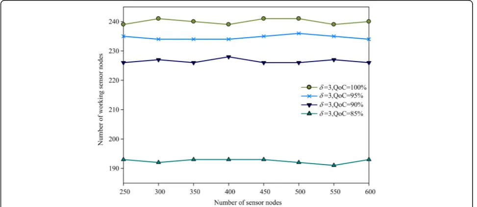
An ideal coverage control algorithm should utilize the minimal number of working nodes to satisfy the desired QoC, which could save the network energy consumption as much as possible. The relationship between the required QoC and the obtained QoC is depicted in Fig. 5 for different number of deployed nodes when δ=3. It can be observed that regardless of the number of deployed nodes, the ENCP could always guarantee the required QoC. Since the number of sensing neighbors is
definitely an integer, the obtained QoC is a little higher than the required QoC. However, the difference between the required and the obtained QoC quickly reduces to 0 as the required QoC increases. Furthermore, it is also impractical to obtain the exact required QoC when the location information is not available.
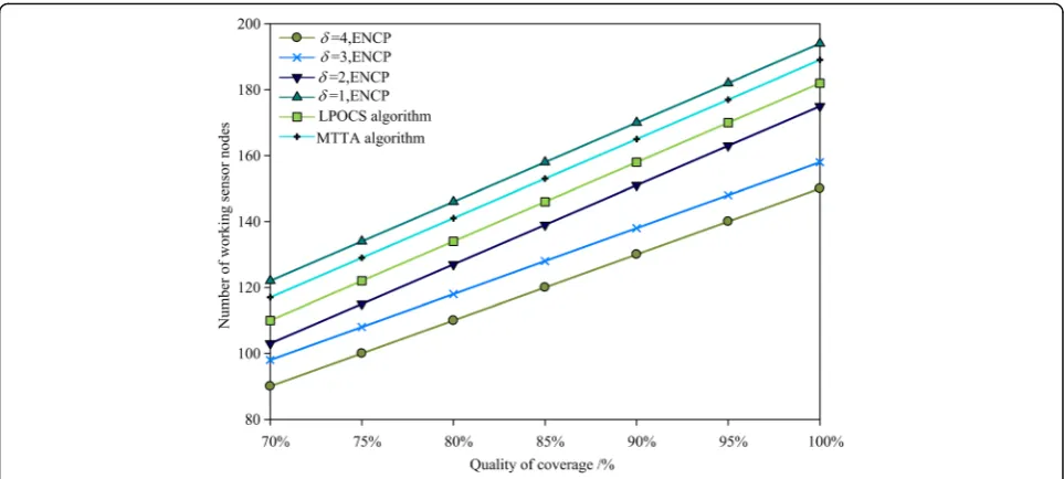
The relationship between the number of working nodes and the number of deployed nodes is depicted in Fig. 6 whenδ= 3. It can be observed from Fig. 6 that the num-ber of working nodes is only related with the desired QoC, instead of the number of deployed nodes. Further-more, the number of working nodes is almost equal to the Fig. 5Relationship between required QoC and obtained QoC whenδ= 3
result calculated according to Eq. (33). This observation verifies the excellent scalability of the ENCP. Although the LDAS [28] shows similar scalability, much more working nodes are needed for the LDAS to guarantee the same QoC. The reason behind this will be explained in Section 4.1. We can also observe from Fig. 6 that more working nodes are required for a higher required QoC.
The relationship between the required QoC and the obtained QoC for different values of δ is depicted in Fig. 7. It can be observe from Fig. 7 that the obtained QoC matches well with the required QoC regardless of the value ofδ. This observation proves that this protocol
can be well applied to any MSNs where the sensing ranges satisfy the normal distribution N (R0, δ2) with
R0≥3.3δ.
To further verify the enhancement of the equalization for the network power, we compare the ENCP with the algorithms in [18, 19]. The simula-tions are performed based on three different sensing fields, and the coverage probability is fixed to 99.9%. The simulation results for different parameters are depicted in Figs. 8, 9, 10, and 11.
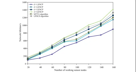
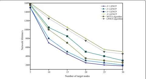
Figures 8, 9, 10, and 11 depict the relationship between the network lifetime and the target nodes within Fig. 7Required QoC and obtained QoC with differentδ
different sensing fields. The algorithms we focus on are the Multiple Target Tracking Algorithm (MTTA) [18] and linear programming optimization coverage scheme (LPOCS) [19]. It can be observed from Fig. 8 that at the initial stages of the program, the network lifetime of the three algorithms increases with the number of nodes. However, due to the limit of the value range of this algo-rithm and the inactive state of the redundant nodes, the network lifetime of the ENCP is lower than the other
algorithms when the equalization is finally achieved for the network energy. During the coverage process for the target node, less network energy is required for the ENCP, which can be explained as above. In Fig. 10, parts of the redundant nodes are transitioned to the state of work due to the increase of the area of the sensing fields. As a result, the network lifetime is prolonged. When
δ = 3, the network lifetime of the ENCP is longer than that of the LPOCS algorithm. When δ = 4, the network Fig. 9100 × 100m2, network lifetime vs the number of target nodes
lifetime of the ENCP is longer than those for both of the other two algorithms. The network lifetime during the coverage for the target node is depicted in Fig. 11. It can be observed that the network lifetime of three algo-rithms decreases with the increase of target nodes. Finally, the energy tends to be equalized. However, the ENCP exhibits a lower decrease speed during the decline process. This is due to the fact that when a part of the sensing field is densely deployed with the sensor nodes, i.e., the coverage expectation is higher for this region, some redundant nodes are awakened via the scheduling mechanism of the sensor nodes. These awakened nodes are transitioned to the state of work to enhance the coverage intensity and further prolong the network lifetime.
6 Conclusions
Focusing on the sensing characteristics of randomly de-ployed MSNs, we analyzed the coverage redundancy problem for the MSNs where the sensing ranges satisfy the normal distribution. We also presented the calcula-tion model for the node redundancy degree for which no location information is needed and the calculation model for the minimal number of working nodes to guarantee the network QoC. According to the analytical result, we proposed the ENCP which shut down all the redundant nodes satisfying the redundancy condition. Based on the ENCP, it enables the collaborative schedul-ing of distributed sensor nodes and balances the energy consumptions of each sensor nodes. The purpose of
energy conservation of the networks is achieved since the ENCP maintains the least number of sensor nodes, as working nodes to provide the desired QoC. Simula-tion results show that the ENCP could not only accur-ately guarantee the desired QoC, but also efficiently reduce the network energy consumption to prolong the effective network lifetime.
Acknowledgements
This work was supported by the National Natural Science Foundation of China under grant no. 61628210, Henan Province Education Department Cultivation Young Key Teachers in University of under grant no. 2016GGJS-158, Henan Province Education Department Natural Science Foundation under grant no. 17A520044, Luoyang Institute of Science and Technology High-level Research Start Foundation under grant no. 2017BZ07, Natural Science and Technology Research of Henan Province Department of Science Foundation under grant no. 162102210113, Guangdong Natural Science Foundation of China under grant no. 2016A030313540, Guangzhou Education Bureau Science Foundation under grant no. 1201430560, Science and Technology Planning Project of Guangzhou under grant no. 201707010284, and Shaanxi Education Bureau Science Foundation under grant no. 2016SF-428. Finally, great thank to the anonymous reviewers for their valuable suggestions to improve the quality of the paper.
Funding
201707010284, and Shaanxi Education Bureau Science Foundation under grant no. 2016SF-428.
Authors’contributions
ZYS and XFX contributed to the conception and algorithm design of the study. ZYS and GZZ contributed to the acquisition of the simulation. All authors contributed to the analysis of the simulation data and approved the final manuscript.
Authors’information
Zeyu Sun received a M.S. and Ph.D degree from Lanzhou University and Xi’an Jiaotong University, in 2010 and 2017. He is an assistant professor in the School of Computer and Information Engineering, Luoyang Institute of Science and Technology, Luoyang, Henan, China. He is a member of China Computer Federation. His research interests lie in wireless sensor networks, parallel computing, mobile computing, and Internet of things (e-mail: [email protected]). Guozeng Zhao received a M.S. degree from Taiyuan University of
Technology in 2010. He is a lecturer in School of Computer and Information Engineering, Luoyang Institute of Science and Technology, Luoyang, China. His research interests include wireless sensor networks and cloud computing (e-mail:[email protected]).
Xiaofei Xing received BS degree in computer science and technology from Henan University of Science and Technology in 2003, and an MS and Ph.D. degrees in Central South University, China, in 2008 and 2012, respectively. He has been a Research Fellow at University of Tsukuba, Japan, and he had been also a post-doctorate researcher in Applied Mathematics. He is an assistant professor in the School of Computer Science and Educational Software, Guangzhou University, Guangzhou, China. His research interests include wireless sensor networks, mobile computing, and network performance analysis (e-mail:[email protected]).
Competing interests
The authors declare that they have no competing interests.
Publisher’s Note
Springer Nature remains neutral with regard to jurisdictional claims in published maps and institutional affiliations.
Author details
1School of Computer Science and Engineering, Luoyang Institute of Science and Technology, Luoyang, China.2Department of Computer Science and Technology, Xi’an Jiaotong University, Xi’an, China.3School of Computer Science and Educational Software, Guangzhou University, Guangzhou, China.
Received: 17 October 2017 Accepted: 2 January 2018
References
1. N Mittal, U Singh, BS Sohi, A stable energy efficient clustering protocol of wireless sensor networks. Wirel. Netw23(6), 1809–1821 (2017). https://doi. org/10.1007/s11276-016-1255-6
2. V Kumar, SB Dhok, R Tripathi, S Tiwari, Cluster size optimization with Tunable Elfes sensing model for single and multi-hop wireless sensor networks. Int. J. Electron.104(2), 312–327 (2017). https://doi.org/10.1080/ 00207217.2016. 1216177
3. Z Zhao, J Willson, L Zaixin, W Weili, Z Xuding, D Dingzhu, Approximating maximum lifetimek-coverage through minimizing weightedk-cover in homogeneous wireless sensor networks. IEEE/ACM Trans. Networking24(6), 3620–3633 (2016). https://doi.org/10.1109/TNET.2016.2531688
4. J Habibi, H Mahboubi, AG Aghdam, Distributed coverage control of mobile sensor networks subject to measurement error. IEEE Trans. Autom.61(11), 3330–3343 (2016). https://doi.org/10.1109/TAC.2016.2521370
5. L Saewoom, K Kiseon, Key renewal scheme with sensor authentication under clustered wireless sensor networks. Electron. Lett.51(4), 368–369 (2015). https://doi.org/10.1049/el.2014.3327
6. AK Idrees, K Deschinkel, M Salomon, C Raphael, Perimeter-based coverage optimization to improve lifetime in wireless sensor networks. Eng. Optim. 48(11), 1951–1972 (2016). https://doi.org/10.1080/0305215X.2016.1145015 7. N Xiong, V Athanasios, L Yang, L Song, Y Pan, K Rajgopal, Y Li, Comparative
analysis of quality of service and memory usage for adaptive failure
detectors in healthcare systems. IEEE J. Sel. Areas Commun.27(4), 495–509 (2009). https://doi.org/10.1109/SAC.2009.090512
8. F Senel, Coverage-aware connectivity-constrained unattended sensor deployment in underwater acoustic sensor networks. Wirel. Commun. Mob. Comput.16(14), 2052–2064 (2016). https://doi.org/10.1002/WCM.2667 9. K Huang, Z Qi, C Zhou, N Xiong, An efficient intrusion detection approach for
visual sensor networks based on traffic pattern learning. IEEE Trans. Syst. Man Cybernetics: Syst.47(10), 2704–2713 (2017) Doi:10.1109 /TSMC.2017.2698457 10. G Mario, B Holger, S Slawomir, Nomographi functions: efficient computation
in clustered Gaussian sensor networks. IEEE Trans. Wirel. Commun.14(4), 2093–2105 (2015). https://doi.org/10.1109/TWC.2014.2380317
11. M Rout, R Roy, Self-deployment of randomly scattered mobile sensors to achieve barrier coverage. IEEE Sensor J.16(18), 6819–6820 (2016). https:// doi.org/10.1109/JSEN.2016.2590572
12. M Ozger, E Fadel, OB Akan, Event-to-sink spectrum-aware clustering in mobile cognitive radio sensor networks. IEEE Trans. Mobile Comput.15(9), 2221–2233 (2016). https://doi.org/10.1109/YMC.2015.2493526
13. D Saha, N Das, Self-organized area coverage in wireless sensor networks by limited node mobility. Innov. Syst. Softw. Eng.12(3), 227–238 (2016). https:// doi.org/10.1007/s11334-016-0277-7
14. Z Sun, Y Zhang, Y Nie, W Wei, J Lloret, H Song, CASMOC: a novel complex alliance strategy with multi-objective optimization of coverage in wireless sensor networks. Wirel. Netw23(4), 1201–1222 (2017). https://doi.org/10. 1007/s 11276-016-1213-3
15. H-H Cho, TK Shih, H-C Chao, A robust coverage scheme for UWSNs using the spline function. IEEE Sensor J.16(11), 3995–4002 (2016). https://doi.org/ 10.1109/JSEN.2015.2429914
16. N Dong, X Ren, W Wang, M Liu, Node scheduling scheme using spatial resolution of wireless sensor networks. J. Comput. Inf. Syst.11(10), 3701– 3708 (2015). https://doi.org/10.12733/jcis14262
17. X Xing, G Wang, j Li, Polytype target coverage scheme for heterogeneous wireless sensor networks using linear programming. Wirel. Commun. Mob. Comput.14(14), 1397–1408 (2014). https://doi.org/10.1002/wcm.2269 18. T Wang, Z Peng, J Liang, W Sheng, MD Zakirul Alam Bhuiyan, Y Cai, J Cao,
Follow targets for mobile tracking in wireless sensor networks. ACM Trans. Sens. Networks12(4), 31.1–31.24 (2016). https://doi.org/10.1145/2968450 19. Z Sun, Y Shu, X Xing, W Wei, H Song, W Li, LPOCS: a novel linear
programming optimization coverage scheme in wireless sensor networks. Ad Hoc & Sens. Wireless Networks33(1-4), 173–197 (2016)
20. Z Bo, E Tong, J Hao, W Niu, G Li, Energy efficient sleep schedule with service coverage guarantee in wireless sensor networks. J. Netw. Syst. Manag.24(4), 834–858 (2016). https://doi.org/10.1007/s10922-015-9361-9 21. ZSW Wu, H Wang, H Chen, Xiaofei, A novel coverage algorithm based on
event-probability-driven mechanism in wireless sensor network. EURASIP J. Wireless Commun. Networking58, 1–16 (2014) Doi: 10. 1186/1687-1499-2014-58
22. Z Sun, R Tao, L Li, X Xing, A new energy-efficient multi-target coverage control protocol using event-driven-mechanism in wireless sensor networks. Internet J. Online Eng.13(2), 53–67 (2017). https://doi.org/10.3991/ijoe.v13 i02.6465 23. G Xing, M Li, T Wang, W Jia, J Huang, Efficient rendezvous algorithms for
mobility-enabled wireless sensor networks. IEEE Trans. Mob. Comput.11(1), 47–60 (2012). https://doi.org/10.1109/TMC.2011.66
24. K Lin, X Tianlang, J Song, Y Qian, Y Sun, Node scheduling for all-directional intrusion detection in SDR-based 3D WSNs. IEEE Sens. J.16(20), 7332–7341 (2016). https://doi.org/10.1109/JSEN.2016.2558043
25. JP Mohanty, C Mandal, C Reade, A Das, Construction of minimum connected dominating set in wireless sensor networks suing pseudo dominating set. Ad Hoc Netwroks42(2), 61–73 (2016). https://doi.org/10. 1016/j.adhoc.2016.02.003
26. HS Aghdasi, M Abbaspour, Energy efficient area coverage by evolutionary camera node scheduling algorithm in visual sensor networks. Soft. Comput. 20(3), 1191–1202 (2016). https://doi.org/10.1007/s00500-014-1582-4 27. S Jamali, M Hatami, Coverage aware scheduling in wireless sensor networks:
an optimal placement approach. Wirel. Pers. Commun.85(3), 1689–1699 (2015). https://doi.org/10.1007/s11277-015-2862-8
28. D Zeng, P Li, S Guo, T Miyazaki, H Jiankun, Y Xiang, Energy minimization in multi-task software-defined sensor networks. IEEE Trans. Comput.64(11), 3128–3139 (2015). https://doi.org/10.1109/TC.2015.2389802
30. C-p Chen, S Mukhopadhyay, C-l Chuang, T-S Lin, M-S Liao, Y-C Wang, J-A Jiang, A hybrid memetic framework for coverage optimization in wireless sensor networks. IEEE Trans. Cybernetics45(10), 2309–2322 (2015). https:// doi.org/10.1109/TCYB.2014.2371139
31. C-F Cheng, C-W Huang, An energy-balanced and timely self-relocation algorithm for grid-based mobile WSNs. IEEE Sensors J.15(8), 4184–4193 (2015). https://doi.org/10.1109/JSEN.2015.2413367
32. Q Gao, W Ma, W Luo, A combinatorial key predistribution scheme for two-layer hierarchical wireless sensor networks. Wirel. Pers. Commun.96(2), 2179–2204 (2017). https://doi.org/10.1007/s11277-017-4292-2
33. G Mali, S Misra, TRAST: trust-based distributed topology management for wireless multimedia sensor networks. IEEE Trans. Comput.65(6), 1978–1991 (2016). https://doi.org/10.1109/TC.2015.2456026
34. H Wang, F Meng, Z Li, Energy efficient coverage conserving protocol for wireless sensor networks. J. Software (China)21(12), 3124–3137 (2010). https://doi.org/10.3724/SP.J.1001.2010.03693
35. X Jing, H Hanwen, H Yang, A Man Ho, S Li, N Xiong, I Muhammad, V Vasilakos Athanasios, A quantitative risk assessment model involving frequency and threat degree under line-of-business services for infrastructure of emerging sensor networks. Sensor17(3), 642 (2017). https://doi.org/10.3390/s17030642
36. S Aamir, L Malrey, L Changhoon, N Xiong, K Suntae, L Youngkeun, K Kangmin, W Seonmi, J Gisung, The protocol design and new approach for SCADA security enhancement during sensors broadcasting system. Multimedia Tools Appl.75(22), 14641–14668 (2016). https://doi.org/10.1007/ s11042-015-3050-2
37. Y Yoon, Y-H Kim, An efficient genetic algorithm for maximum coverage deployment in wireless sensor networks. IEEE Trans. cybernetics43(5), 1473–1483 (2013). https://doi.org/10.1109/TCYB.2013.2250955 38. J Zhang, X Li, S Zhou, X Ye, A novel sleep scheduling scheme in green
wireless sensor networks. J. Supercomuting71(3), 1067–1094 (2015). https:// doi.org/10.1007/s11227-014-1354-z
39. S Wang, H Yi, L Wu, F Zhou, NN Xiong, Mining probabilistic representative gathering patterns for mobile sensor data. J. Internet Technol.18(2), 321– 332 (2017). https://doi.org/10.6138/JIT.2017.18.2.20161125
40. J-W Lee, B-S Choi, J-j Lee, Energy-efficient coverage of wireless sensor networks using ant colony optimization with three types of pheromones. IEEE Trans. Ind. informatics7(3), 419–427 (2011). https://doi.org/10.1109/TII. 2011.21588 36
41. H Mohamadi, AS Ismail, S Salleh, Solving target coverage problem using cover sets in wireless sensor networks based on learning automata. Wirel. Pers. Commun.75(1), 447–463 (2014). https://doi.org/10.1007/s11277-013-1371–X
42. H Cheng, S Zhihuang, N Xiong, X Yang, Energy-efficient node scheduling algorithm for wireless sensor networks using Markov random field model. Inf. Sci.329(2), 461–477 (2016). https://doi.org/10.1016/j.ins.2015.09.039 43. P Chen, W Hu, Sleep-wake up scheduling with probabilistic coverage model in
sensor networks. International Journal of Parallel, Emergent and Distributed Syst.29(1), 1–16 (2014). https://doi.org/10.1080/17445760.2013.766733 44. B Bae, J Park, S Lee, A free market economy model for resource management
in wireless sensor networks. Wireless Sens. Networks7(6), 76–82 (2015). https:// doi.org/10.4236/wsn.2015.76007
45. L Zaixin, WW Li, M Pan, Maximum lifetime scheduling for target coverage and data collection in wireless sensor networks. IEEE Trans. Vehicular Technol.64(2), 714–727 (2015). https://doi.org/10.1109/TVT.2014.2322356 46. N Xiong, RW Liu, M Liang, W Di, Z Liu, W Huisi, Effective alternating