A new approach to estimating a numerical solution in the error embedded correction framework

(1)

R E S E A R C H

Open Access

A new approach to estimating a numerical

solution in the error embedded correction

framework

Philsu Kim

1

_{, Xiangfan Piao}

2

_{, WonKyu Jung}

3

_{and Sunyoung Bu}

4*

*_{Correspondence:}

[email protected] 4_{Departments of Liberal arts,}

Hongik University, Sejong, Korea Full list of author information is available at the end of the article

Abstract

On the basis of the error correction method developed recently, an algorithm, so-called error embedded error correction method, is proposed for initial value problems. Two deferred equations are used to approximate the solution and the error, respectively, at each integration step. For the solution, the deferred equation, which is based on a modiﬁed Euler’s polygon including the information of both the solution and its estimated error at the previous integration step, is solved with the classical fourth-order Runge–Kutta method. For the error, the deferred equation, which is based on a local Hermite cubic polynomial with three pieces of information—the solution, its estimated error at the previous step, and the constructed solution—is solved by the seventh-order Runge–Kutta–Fehlberg method. The constructed algorithm controls the error and possesses a good behavior of error bound in a long time simulation. Numerical experiments are presented to validate the proposed algorithm.

Keywords: Error correction method; Runge–Kutta method; Runge–Kutta–Fehlberg

method; Long time simulation; Initial value problem

1 Introduction

There are many research topics [1, 2] in developing numerical methods for solving initial value problems (IVPs) described by

dφ dt =f

t,φ(t), t∈[t0,tf]; φ(t0) =φ0, (1) wheref has continuously bounded partial derivatives up to required order for the analy-sis of the developed numerical method. A long time simulation of the solution, which is needed in many physical problems (for example, a Hamiltonian system such as the Kepler problem, harmonic oscillator, molecular dynamics, etc.), is one of the most important top-ics in IVPs [3–5]. Also, such long time simulations sometimes demand very special step size selection to control the local truncation error. Most existing mechanisms of the ex-plicit single step algorithm for solving (1) may be described by

⎧ ⎨ ⎩

φm+1=F(φm), em+1=G(φm,φm+1),

(2)

whereFandGare functions derived from the numerical methods. Here,φm+1andem+1 de-note the approximations of the solution and the local truncation errorEm+1, respectively, at timetm+1. For apth order scheme, the estimated errorem+1is usually approximated to fit only the coefficient of the (p+ 1)th order term in the expansion ofEm+1about the time step sizeh. The other important issue is to reduce the computational costs in a long time simulation, for which an efficient control scheme of the time step size is important (for example, Radau5). There have been several approaches related to those issues (for exam-ple, embedded Runge–Kutta formulae, adaptive time stepping, long time error estimation, etc. [6–11]).

In the existing schemes, the estimated errorem obtained from the previous time step [tm–1,tm] is mainly used only for choosing an appropriate next time step size in most al-gorithms. Also, the solutionφm+1at timetm+1is calculated with an initial value which is a solutionφmat the previous timetm. That is,φmis assumed to be the exact initial condition forφm+1despite the existence of the local truncation errorem, which leads to accumulation of the error as the time is increasing. In order to control the accumulation error, smaller integration steps or special step size controllers are sometimes required, especially for a long time simulation or stiﬀ systems. Nevertheless, the most existing methods cannot fully resolve the error control to get a given tolerance so that it is diﬃcult to get reliable results at stringent tolerances (for example, see [12, 13]).

The subject of this paper is to develop a new integration scheme to control the accu-mulation error. As a remedy to control or minimize the accumulated error ofem, we will embed it in the algorithm of the calculation scheme forφm+1. Further, we want to propose an estimating scheme forem+1 which is correlated with three pieces of informationφm, φm+1, andem. That is, the scheme we want to develop is an explicit single step algorithm, the so-called error embedded error correction method (EEECM), of the form

⎧ ⎨ ⎩

φm+1=F(φm,em), em+1=G(φm,em,φm+1).

(3)

To concretely describe the proposed algorithm, the classical 4th order Runge–Kutta (RK4) method and the well-known 7th order Runge–Kutta–Fehlberg (RKF7) method for calcu-latingφm+1 andem+1, respectively, will be used. Finally, we want to develop the EEECM having the accuracy order of 7 for the solutionφ˜m+1=φm+1+em+1. In particular, we will develop the efficient estimating algorithm forem+1, which fits the coefficients up to 7th order term in the expansion of the global errorEm+1=φ(tm+1) –φm+1about the time step sizeh.

An error correction method (ECM) is a widely used technique in many numerical sci-entiﬁc computations in general. The deferred correction methods (DCM) originally de-veloped by Pereyra and Zadunaisky [14, 15] are the representative ECMs for solving (1). There are also extended results about the DCMs (for example, see [16–24]). These ECMs are based on the deferred equation of the form

dψ(t) dt =f

(3)

wherexis a local approximation of the solution deﬁned on each integration step [tm,tm+1]. After solving (4), the solutionφ(t) of (1) can be obtained by using the identity

φ(t) =x(t) +ψ(t). (5)

Two relations (4) and (5) enable us to develop the EEECM of the form (3) for solving (1). Practically, for the approximate solutionφm+1, we use a local linear approximationxwhich uses the information of both the solution and its slope depending on the erroremat time tm and solve the deferred equation (4) with RK4. As mentioned above, we want to esti-mate the exact quantity of the errorEm+1up to the desired convergence order. To derive a formula forem+1, another local approximationxis constructed by a local Hermite cu-bic interpolation polynomial having all the information of the calculated solutions and those slopes at both timetmandtm+1. Based on the local approximation, we again solve the deferred equation (4) with the RKF7. As an appropriate step size controller, we ex-ploit a standard step size controller to focus only on the EEECM for non-stiff problems. The constructed EEECM controls the error at each integration step, and it turns out that the proposed method possesses a good behavior of error bound in a long time simulation with a given tolerance. For an assessment of the effectiveness of the proposed algorithm, particularly its error bounds in a long time simulation, a simple harmonic oscillator prob-lem with analytical solution and a hard error controlling probprob-lem are numerically solved. Finally, a two-body Kepler problem is also used to assess the efficiency of this algorithm. Throughout these numerical tests, it is shown that the proposed method is quite efficient compared to several existing methods.

This paper is organized as follows. In Sect. 2, we describe the methodology to formulate and control the solution and error formulas based on ECM. In Sect. 3, we give a concrete analysis of the convergence for the developed EEECM. Several numerical results are pre-sented in Sect. 4 to give both the numerical evidences for the theoretical analysis and the numerical eﬀectiveness of EEECM. Finally, in Sect. 5, a summary for EEECM and some discussion for further works are given.

2 Derivation of algorithm

In this section, we present the algorithm of EEECM based on the deferred equations. Let us assume that the approximated solutionφmand the estimated erroremfor the solution φ(tm) and the errorEm, respectively, at timetm are already calculated. Then, as a local approximation of the solutionφ(t) on the integration step [tm,tm+1], one may consider the modiﬁed Euler’s polygony(t) deﬁned by

y(t) :=φm+ (t–tm)f(tm,φm+em), t∈[tm,tm+1]. (6)

Letψ(t) be the diﬀerence betweenφ(t) andy(t) such that

(4)

Differentiating both sides of (7) and combining the result with (1) and (6), one can see that the differenceψ(t) satisfies the following deferred differential equation:

⎧ ⎨ ⎩

ψ(t) =g1(t,ψ(t)), t∈(tm,tm+1], ψ(tm) =Em,

(8)

whereg1is deﬁned by

g1

t,ψ(t):=ft,ψ(t) +y(t)–y(t) =ft,ψ(t) +y(t)–f(tm,φm+em). (9)

Observe that the initial conditionψ(tm) of (8) is given by the unknown actual errorEm at timetm, and hence problem (8) cannot be solved directly. Sinceemis assumed to be an estimated error ofEm=ψ(tm), instead of solving (8), it is natural to consider the following IVP:

⎧ ⎨ ⎩

θ(t) =g1(t,θ(t)), t∈(tm,tm+1], θ(tm) =em

(10)

for an approximation ofψ(tm+1). One may check that applying RK4 to (10) leads to

θ(tm+1)≈em+ h

6[–5v1+ 2v2+ 2v3+v4],

v1=f(tm,φ˜m), v2=f

tm+ h 2,φ˜m+

h 2v1

,

v3=f

tm+ h 2,φ˜m+

h 2v2

, v4=f(tm+h,φ˜m+hv3),

(11)

where φ˜m :=φm+em. Combining approximation (11) with (6) and (7), one may get an approximation formula forφ(tm+1) as follows.

φm+1:=φ˜m+ h

6[v1+ 2v2+ 2v3+v4], (12)

where the intermediate values vi are deﬁned by (11). Note that the classical RK4 uses only the approximate valueφmat timetmto calculateφm+1, whereas algorithm (12) uses the valueφ˜m:=φm+eminstead ofφm, which is a remarkable diﬀerence compared to the RK4.

Since the estimated erroremat timetmis embedded in algorithm (12), a recursive rela-tion for a sequence{em}is needed to complete the algorithm. We try to derive this relation using another deferred equation together with an appropriate local approximation. Recall that after the calculation of (12), one can use the information of both the approximate solutions and those slopes at timetm andtm+1. Hence, as the local approximation, it is natural to use a local Hermite cubic interpolation such that

(5)

satisfyingx(tm) =φ˜m,x(tm) =f(tm,φ˜m),x(tm+1) =φm+1, andx(tm+1) =f(tm+1,φm+1). Then it solves [25]

x(t) =x(tm) +x(tm)(t–tm) +

x(tm+1) –x(tm) –x(tm)h h2 (t–tm)

2

+(x ₍_t

m+1) +x(tm))h– 2(x(tm+1) –x(tm)) h3 (t–tm)

2₍_t_–_t

m+1). (14)

Letψ(t) be the diﬀerence betweenφ(t) andx(t) such that

ψ(t) :=φ(t) –x(t), t∈[tm,tm+1]. (15)

As the derivation of (8), one can see that the differenceψ(t) defined by (15) satisfies the following deferred differential equation:

⎧ ⎨ ⎩

ψ(t) =g2(t,ψ(t)), t∈(tm,tm+1], ψ(tm) =Em–em,

(16)

whereg2is deﬁned by

g2

t,ψ(t):=ft,ψ(t) +x(t)–x(t). (17)

Observe that the initial conditionψ(tm) of (16) contains the unknown valueEmand hence problem (16) cannot be solved directly. Sinceemis the estimated error ofEm, if one as-sumes that it is well approximated, then the initial valueψ(tm) becomes quite small. Hence, instead of solving (16), it is natural to consider the following IVP:

⎧ ⎨ ⎩

θ(t) =g2(t,θ(t)), t∈(tm,tm+1], θ(tm) = 0

(18)

for an approximation ofψ(tm+1). To solve (18), we consider the well-known RKF7 with Butcher array [26]

c A

bT, (19)

where

c= [c1,c2, . . . ,c11]T:= 0, 2 27,

1 9,

1 6,

5 12,

1 2,

5 6,

1 6,

2 3,

1 3, 1

T ,

b= [b1,b2, . . . ,b11]T:= 41

840, 0, 0, 0, 0, 34 105,

9 35,

9 280,

41 840

T

(6)

A= (αi,j) :=

From the deﬁnition of the Hermite interpolation x deﬁned by (14), one may see that ψ(tm+1) =φ(tm+1) –φm+1:=Em+1. Also, we recall that system (18) is a perturbed system

It is easy to check that the coeﬃcients (20) in Butcher array (19) have the following identities:

(7)

Lemma 1 The algorithm for em+1deﬁned by(22)can be simpliﬁed by

em+1=φm+em–φm+1+h 11

i=1

biVi, (24)

where the intermediate values Viare deﬁned by

V1:=v1, V2:=f

tm+c2h,x(tm+c2h)

,

Vi:=f

tm+cih,φm+em+h i–1

j=1 αi,jVj

, i= 3, . . . , 11,

(25)

where v1is deﬁned by(11).

Proof For the quantityKideﬁned by (21), we let

i:=Ki+x(tm+cih), i= 2, 3, . . . , 11.

Then algorithm (22) can be written as

em+1=γ +h 11

i=2 bii,

2=f

tm+c2h,x(tm+c2h)

,

i=f

tm+cih,h i–1

j=2

αi,jj+βi

, i= 3, . . . , 11,

(26)

whereγ andβiare deﬁned by

γ := –h 11

i=2

bix(tm+cih),

βi:= –h i–1

j=2

αi,jx(tm+cjh) +x(tm+cih).

(27)

For a simpliﬁcation ofγ andβideﬁned in (27), we consider Taylor’s expansion ofxabout t=tmgiven by

x(t) =x(tm) + (t–tm)x(tm) +

(t–tm)2

2 x

₍_t m) +

(t–tm)3

6 x

(3)₍_t

m). (28)

By substituting (28) into the formula ofγ given in (27) and combining the result with (23) and (28), one may check that

γ =hb1x(tm) –hx(tm) – h2

2 x ₍_t

m) – h3

6x (3)₍_t

m)

(8)

and

βi=x(tm) +hαi,1x(tm), i= 3, . . . , 11. (30)

Hence, substituting (29) and (30) into (26) and considering the deﬁnition ofVideﬁned by

(25), one can complete the proof.

Remark1 Remark that 16 evaluations of the Hermite interpolation and its derivatives are required for algorithm (22). However, by introducing Lemma 1, only one evaluation of the Hermite interpolation is required. It is remarkable.

For summarizing the algorithm we discussed, we consider the Butcher array of RK4 given by

nS

k, (31)

where

n= [n1,n2,n3,n4] := 0,1 2,

1 2, 1

, k= [k1,k2,k3,k4] := 1 6,

1 3,

1 6

,

S= (si,j) := ⎡ ⎢ ⎢ ⎢ ⎣

0 0 0 0 1

2 0 0 0 0 1₂ 0 0 0 0 1 0 ⎤ ⎥ ⎥ ⎥ ⎦.

(32)

Also, if we deﬁne

V0:=f(tm+1,φm+1),

then, from the deﬁnition ofxgiven in (14), we have

x(tm+c2h) =φm+em+ (φm+1–φm–em)c22(3 – 2c2)

+c2(1 –c2)h(1 –c2)V1–c2V0

.

Thus, by combining it with (24) and (12), one can derive the algorithm EEECM given by ⎧

⎨ ⎩

φm+1=φm+em+h4i=1kivi, em+1=φm+em–φm+1+h

11 i=1biVi,

m≥0, (33)

where the intermediate valuesviandViare deﬁned by

v1=f(tm,φm+em), vi=f(tm+nih,φm+em+hsi,i–1vi–1), i= 2, 3, 4,

V0=f(tm+1,φm+1), V1=v1,

V2=f

(9)

Figure 1Geometric meaning of the error embedded error correction methods

+c2(1 –c2)h(1 –c2)V1–c2V0

,

Vi=f

tm+cih,φm+em+h i–1

j=1 αi,jVj

, i= 3, . . . , 11.

Also, if we letφ˜m:=φm+em, then one may get a better approximation{ ˜φm}than the ap-proximation{φm}, and it satisﬁes the following recurrence relation:

˜

φm+1=φ˜m+h 11

i=1

biVi, m≥0, (35)

where the intermediate valuesViare calculated by

v1=f(tm,φ˜m), vi=f(tm+nih,φ˜m+hsi,i–1vi–1), i= 2, 3, 4,

V0=f

tm+1,φ˜m+h 4

i=1 kivi

, V1=v1,

V2=f

tm+c2h,φ˜m+c22(3 – 2c2)h 4

i=1

kivi+c2(1 –c2)h

(1 –c2)V1–c2V0

,

Vi=f

tm+cih,φ˜m+h i–1

j=1 αi,jVj

, i= 3, . . . , 11.

(36)

Remark2 The algorithm of EEECM (33) (or (35)) needs 15 function evaluations in each time step, which is two more function evaluations than those of RKF78. Unlike RKF78, not only is the estimated error sequence{em}embedded to calculate the solutionφm, but also it will be used to control the time step size. This is the reason why we call the proposed algorithm an error embedded error correction method. We also remark that scheme (33) (or (35)) is also applicable to a system of ODEs of the form

₍_t_{) =}_F_t_,₍_t₎_, _t_∈₍_t_0,_t

f]; (t0) = 0,

where := [φ1(t), . . . ,φd(t)]TandF:= [f1(t, (t)), . . . ,fd(t, (t))]T.

(10)

attm+1based on the deferred equation constructed by the Euler polygony(t), for which two pieces of informationφmandemcalculated at timetmare used. To complete the algorithm, a scheme embedding the sequence of the estimated erroreminto the algorithm itself is required. Therefore, in the second step, the local truncation errorEm+1is estimated with another deferred equation based on higher order local approximationx(t), for which all pieces of informationφm,φm+1, andemare used.

3 Convergence analysis

The aim of this section is to give a concrete convergence analysis for algorithm (35). For the simplicity of the analysis, we assume that IVP (1) is an autonomous problem. That is, we assumef(t,φ(t)) :=f(φ(t)). For a simpliﬁcation, we introduce the operatorDk_deﬁned

The above two relations (39) and (40) give a simple expansion ofXias follows.

(11)

+h

where all the functions on the right-hand side are evaluated at the value y and(a)idenotes the ith component of a vectora.Here, c0_{:= [1, 1, . . . , 1]}T_{and also a multiplication between} the above vector multiplication. To obtain a series expansion ofXiin terms ofh, we let

X:= by Taylor’s expansion ofX3 in terms ofh. Further, we expand the resulted equation in ascending order ofh. Then one may check that fori≥4,

Thus, by comparing the coeﬃcients of two equations (43) and (44), one may have the following recurrence relations for ai:

(12)

(a5)i=

Finally, we solve the recurrence relations (45) with the aid of the relations in (23) and (37). Then one may get the required identity in (41).

From equation (39) together with (41) in the above lemma, we have the following corol-lary.

Corollary 1 For the intermediate values Vi(i≥6)deﬁned in(38),we have

Vi=

Proof By directly substituting (41) into (39) and expanding the resulted equation in

as-cending order ofhwith the aid of the identity (Ac3)i=

c4_i

4,i≥6, one may get the required

equation (46).

Substituting expansion (46) into the sum of F deﬁned by (38) leads to the following theorem.

Theorem 1 Let us assume that the slope function f is suﬃciently smooth.Then the function

F deﬁned by(38)satisﬁes

F(y,h;f) =

Proof By substituting the expansion ofViin (46) into the sum ofFin (38) and simplifying the result, one may get

(13)

+f

From the Butcher array (19) with the coeﬃcients in (20), one may check that

11

Combining the relations in (49) with equation (48) yields the required equation (47).

For a concrete convergence analysis of scheme (35), similar to the methodology in [25], we now deﬁne the truncation error by

Tm(φ) :=φ(tm+1) –φ(tm) –hF

Then two equations (50) and (51) give

φ(tm+1) =φ(tm) +hF

φ(tm),h;f

+hτm(φ), m≥0. (52)

Thus, subtract (35) from (52) together with (38) to obtain

˜ that the functionFsatisﬁes a Lipschitz condition

F(y,h;f) –F(z,h;f)≤L|y–z| (54)

for all –∞<y,z<∞and all smallh> 0. This condition can be usually obtained by using the Lipschitz condition onf and its derivatives. Applying the Lipschitz condition (54) into (53) leads to

| ˜Em+1| ≤(1 +Lh)| ˜Em|+hτ(h), m≥0, (55)

whereτ(h) is deﬁned by

τ(h) =max

(14)

On the other hand, from Taylor’s expansion ofφ(tm+1) abouttm and two equations (47) and (50), one may get

τm(φ) =O

h7, m≥0, (57)

for a suﬃciently smooth functionf. Hence, from the above three relations (55), (56), and (57), one can get the following convergence theorem for algorithm (35).

Theorem 2 Assume that the present method(35)satisﬁes the Lipschitz condition(54)and the slope function f is suﬃciently smooth.Then,for the IVP(1),algorithm(35)has the rate of convergenceO(h7_).

Remark4 Theorem 2 shows that the estimated errorem+1in algorithm (33) exactly esti-mates the coeﬃcients of Taylor’s expansion abouthof the errorEm+1:=φ(tm+1) –φm+1up to the 7th order term, whereas the embedded RKF78 exactly estimates the 8th order term only. Also, unlike the existing embedded schemes, the estimated erroremis embedded in the algorithm EEECM itself by considering as an initial value at each time interval. It turns out that the proposed algorithm (33) is more eﬃcient in a long time simulation, which is shown throughout several numerical results (see Sect. 4).

4 Numerical results

In this section, we show several numerical results and compare the eﬃciency of the pro-posed method to those of other existing methods such as BV78, RKF78, Radau5, and Mat-lab built-in routines—ode113 and ode45 [2, 26, 27]. As a time step control for the proposed method, we use a standard step size selection algorithm (for example, [1, 28]) which is given by

hm+1=

tol

em∞ 1

5

hm, (58)

wheretolis a given tolerance andem is the estimated local truncation error at timetm calculated by (33). Also, the initial time step size is chosen byh0=1₄(tol)

1

5_{, since RK4 is}

used to approximate the solution. In each test problem, we calculate both errors Em= φ(tm) –φmandE˜m=φ(tm) –φm–emdenoted by EEECM and EEECM(e), respectively.

4.1 Simple problems

In this subsection, we will show the eﬃciency of EEECM with two simple IVPs. One is a well-known simple harmonic oscillator. The other is knowing that the global error control is quite diﬃcult [12]. Details of each problem will be explained in each subsection.

Example1 Consider a harmonic oscillator described by

⎧ ⎨ ⎩

y₁(t) = –y2(t),

y2(t) =y1(t),

(59)

(15)

Table 1 Convergence order of EEECM for solving a simple harmonic oscillator

Step-size Error Rate

0.5 2.7007e–006

0.25 1.8878e–008 7.160437 0.125 1.3484e–010 7.129298 0.0625 9.9618e–013 7.080680 0.03125 7.0429e–015 7.144086

Figure 2Comparison of the error with diﬀerent tolerances (a)tol= 1e–6 (b)tol= 1e–8

To validate the theoretical convergence analysis in Theorem 2, the problem is solved on the interval [0, 500] with different step sizes and the results are reported in Table 1. The first column shows time step sizes, the second does the errors measured by sup norm at the final time, and the last gives the rates between the errors generated by using the previous and the current step sizes. The results show that the numerical convergence order is 7, which validates theoretical convergence order.

For a demonstration of a long time simulation of EEECM, we solve the problem on the interval [0, 105_{] and show how solutions and errors are well calculated. In Fig. 2, we plot} the absolute errors in a log scale calculated by various numerical schemes with two dif-ferent tolerances (a) 1e–6 and (b) 1e–8. It can be seen that all existing methods have the exponential growth of the error in the sense that the errors over time are increasing lin-early up in a log scale. On the other hand, the ﬁgures of EEECM have uniform-like error bound during the whole time interval under the given tolerances. Furthermore, the results of EEECM(e) are superior to those of the existing methods. These remarkable results may contribute to many other ﬁelds which stood in needs of long-term simulations.

(16)

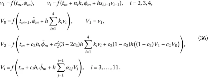
Figure 3Comparison of errors versus CPU-times for given tolerances from 1e–5 to 1e–10

conclude that the proposed method is the most eﬃcient scheme in view of the above dis-cussion, restricted to this harmonic oscillator problem.

Example2 In this example, we test a system that the global error control task becomes more diﬃcult [12] as the time goes on. The system consists of four equations given by

⎧ ⎪ ⎪ ⎪ ⎪ ⎪ ⎨ ⎪ ⎪ ⎪ ⎪ ⎪ ⎩

y1= 2ty21/5y4,

y₂= 10texp(5(y3– 1))y4,

y₃= 2ty4,

y₄= –2tlog(y1)

(60)

deﬁned on the interval [0, 20] with the initial conditiony(0) = [1, 1, 1, 1]T_{. Its analytic} so-lutions are given by

y1(t) =expsint2, y2(t) =exp5sint2,

y3(t) =sint2+ 1, y4(t) =cost2.

(61)

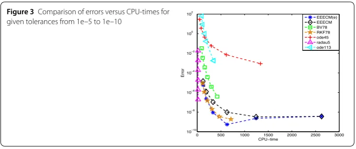
The derivatives of the system show that their oscillation frequencies grow up rapidly when the time goes on. This is the reason why the global error control task [12] is difficult. We solve the problem with a fixed tolerancetol= 1e–8 and plot the absolute error in a log scale in Fig. 4(a). One can see that the proposed method achieves the required accuracy within the given tolerance on the interval [0, 20], whereas all other methods fail to meet the given tolerances and some results at the final time are significantly contaminated by the errors.

(17)

Figure 4Comparison of (a) the error with a given tolerancestol= 1e–8 and (b) errors versus CPU-times for given tolerances from 1e–5 to 1e–10

4.2 Hamiltonian system

Formally, a Hamiltonian system is a dynamical system completely described by the scalar functionH, the Hamiltonian. Firstly, we solve a simple pendulum problem to show how well EEECM can conserve the total energyH. Secondly, we test a two-body Kepler prob-lem to conﬁrm that the proposed method is well ﬁt for the Hamiltonian system.

4.2.1 Pendulum problem

In this example, we solve the equation for the period of swing of a simple gravity pendulum depending only on its length and the local strength of gravity. The total energy of the pendulum is given by

H(p,q) =1 2p

2_–_cos(_q_), ₍₆₂₎

whose componentspandqsatisfy ⎧

⎨ ⎩

p(t) =sin(q),

q(t) =p. (63)

We solve the system on the interval [0, 500] with the initial conditionsp(0) = 1 andq(0) =π 2 together with the given tolerance 1e–8. We examine the conservation property of the total energyHdescribed by|H(p(0),q(0)) –H(pm,qm)|=|1₂–H(pm,qm)|, wherepmandqmare the approximate solutions at timetm. The numerical results are reported in Fig. 5 and show that only three methods, ode113, RKF78, and EEECM, achieve the invariance ofHwithin the given tolerances. In particular, the numerical result of EEECM(e) has an outstanding conservation property compared to other numerical results. Hence, one may claim that the proposed method is superior to other existing methods.

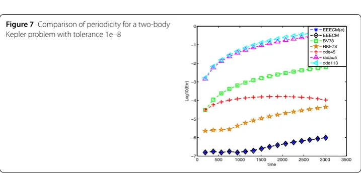
4.2.2 Kepler problem

(18)

Figure 5Comparison of invariance of the total energyHfor solving the pendulum problem with tolerance 1e–8

the (q1,q2)-plane [29]. Assuming unitary masses and gravitational constant, the dynamics is described by the Hamiltonian functionHgiven by

H(p1,p2,q1,q2) = 1 2

p2₁+p2₂– 1 q2

1+q22

(64)

together with the angular momentumL, which is another invariant of the system, de-scribed by

L(p1,p2,q1,q2) =q1p2–q2p1, (65)

whose componentspi,qi(i= 1, 2) satisfy the following IVP:

⎧ ⎪ ⎪ ⎪ ⎪ ⎪ ⎨ ⎪ ⎪ ⎪ ⎪ ⎪ ⎩

p₁(t) = –q1(q12+q22)(–3/2),

p₂(t) = –q2(q12+q22)(–3/2),

q₁(t) =p1,

q₂(t) =p2.

(66)

We solve system (66) with the initial conditionsp1(0) = 0,p2(0) = 2,q1(0) = 0.4,q2(0) = 0 on the interval [0, 1000π] together with a ﬁxed tolerance 1e–8. It is well known that the true solution is periodic with periodicity 2π[30]. As the previous example, we examine the conservation properties of the total energyH(Fig. 6(a)) as well as the angular momentum L(Fig. 6(b)). From the two ﬁgures, one can see that the numerical results EEECM(e) are the most accurate.

(19)

Figure 6The invariances of (a) total energyHand (b) angular momentumLfor a two-body Kepler problem with tolerance 1e–8

Figure 7Comparison of periodicity for a two-body Kepler problem with tolerance 1e–8

5 Conclusion and further discussion

A new error control strategy for non-stiﬀ problems is developed within the ECM frame-work. Unlike the traditional way to approximate solutions in an explicit single step method, we suggest a methodology that contains the estimated error at each integration step and enables us to control the bound of the local truncation error for a long time simulation. Throughout several numerical results, it is shown that the proposed method obtains a uniform-like error bound, which is outstanding compared with existing numeri-cal methods. Also, it is seen that like symplectic methods, the proposed scheme preserves the invariants such as the energy and angular momentum in Hamiltonian systems.

(20)

Acknowledgements

The authors would like to express their gratitude to the reviewers and the editor for valuable suggestions and comments.

Funding

The ﬁrst author Kim was supported by the Basic Science Research Program through the National Research Foundation of Korea (NRF) funded by the Ministry of Education, Science and Technology (grant number 2016R1A2B2011326). Also, the corresponding author Bu was supported by the Basic Science Research Program through the National Research Foundation of Korea (NRF) funded by the Ministry of Education, Science and Technology (grant number

2016R1D1A1B03930734). The second author Piao was supported by the Basic Science Research Program through the National Research Foundation of Korea (NRF) funded by the Ministry of Science, ICT and Future Planning (grant number 2017R1C1B1002370).

Competing interests

The authors declare that they have no competing interests.

Authors’ contributions

PK and XP provided the basic idea of this work and developed all theory needed in this manuscript. WJ simulated the numerical examples, and the corresponding author SB completed the proofs for all the theorems in this manuscript and wrote the manuscripts. All authors read and approved the ﬁnal manuscript.

Author details

1_{Department of Mathematics, Kyungpook National University, Daegu, Korea.}2_{Department of Mathematics, Hannam}

University, Daejeon, Korea. 3_{Dongwoo Fine Chem, Pyeongtaek, Korea.}4_{Departments of Liberal arts, Hongik University,} Sejong, Korea.

Publisher’s Note

Springer Nature remains neutral with regard to jurisdictional claims in published maps and institutional aﬃliations.

Received: 18 September 2017 Accepted: 26 April 2018

References

1. Hairer, E., Norsett, S.P., Wanner, G.: Solving Ordinary Diﬀerential Equations. I Nonstiﬀ. Springer Series in Computational Mathematics. Springer, Berlin (1993)

2. Hairer, E., Wanner, G.: Solving Ordinary Differential Equations. II Stiff and Differential-Algebraic Problems. Springer Series in Computational Mathematics. Springer, Berlin (1996)

3. Calvo, M.P., Hairer, E.: Accurate long-term integration of dynamical systems. Appl. Numer. Math.18, 95–105 (1995) 4. Hairer, E.: Long-time integration of non-stiﬀ and oscillatory Hamiltonian systems. AIP Conf. Proc.1168(1), 3–6 (2009) 5. Tiwari, S., Kumar, M.: An initial value technique to solve two-point non-linear singularly perturbed boundary value

problems. Appl. Comput. Math.14(2), 150–157 (2015)

6. Dormand, J.R., Prince, P.J.: A family of embedded Runge–Kutta formulae. J. Comput. Appl. Math.6(1), 19–26 (1980) 7. Estep, D.: A posteriori error bounds and global error control for approximation of ordinary diﬀerential equations. SIAM

J. Numer. Anal.32(1), 1–48 (1995)

8. Gustafsson, K.: Control-theoretic techniques for stepsize selection in implicit Runge–Kutta methods. ACM Trans. Math. Softw.20(4), 496–517 (1994)

9. Johnson, C.: Error estimates and adaptive time-step control for a class of one-step methods for stiﬀ ordinary diﬀerential equations. SIAM J. Numer. Anal.25(4), 908–926 (1988)

10. Kavetski, D., Binning, P., Sloan, S.W.: Adaptive time stepping and error control in a mass conservative numerical solution of the mixed form of Richards equation. Adv. Water Resour.24, 595–605 (2001)

11. Kulikov, G.Y.: Global error control in adaptive nordsieck methods. SIAM J. Sci. Comput.34(2), 839–860 (2012) 12. Kulikov, G.Y., Weiner, R.: Global error estimation and control in linearly-implicit parallel two-step peer W-methods.

Comput. Appl. Math.236, 1226–1239 (2011)

13. Shampine, L.F.: Error estimation and control for ODEs. J. Sci. Comput.25(1), 3–16 (2005)

14. Pereyra, V.: Iterated deferred correction for nonlinear boundary value problems. Numer. Math.11, 111–125 (1968) 15. Zadunaisky, P.E.: On the estimation of errors propagated in the numerical integration of ordinary diﬀerential

equations. Numer. Math.27, 21–40 (1976)

16. Bu, S., Huang, J., Minion, M.L.: Semi-implicit Krylov deferred correction methods for diﬀerential algebraic equations. Math. Comput.81(280), 2127–2157 (2012)

17. Bu, S., Lee, J.: An enhanced parareal algorithm based on the deferred correction methods for a stiﬀ system. J. Comput. Appl. Math.255(1), 297–305 (2014)

18. Dutt, A., Greengard, L., Rokhlin, V.: Spectral deferred correction methods for ordinary diﬀerential equations. BIT Numer. Math.40(2), 241–266 (2000)

19. Huang, J., Jia, J., Minion, M.L.: Accelerating the convergence of spectral deferred correction methods. J. Comput. Phys.

214(2), 633–656 (2006)

20. Huang, J., Jia, J., Minion, M.L.: Arbitrary order Krylov deferred correction methods for diﬀerential algebraic equations. J. Comput. Phys.221(2), 739–760 (2007)

21. Kim, P., Piao, X., Kim, S.D.: An error corrected Euler method for solving stiﬀ problems based on Chebyshev collocation. SIAM J. Numer. Anal.49, 2211–2230 (2011)

22. Kim, S.D., Piao, X., Kim, D.H., Kim, P.: Convergence on error correction methods for solving initial value problems. J. Comput. Appl. Math.236(17), 4448–4461 (2012)

23. Kim, S.D., Kim, P.: Exponentially ﬁtted error correction methods for solving initial value problems. Kyungpook Math. J.

(21)

24. Kim, P., Lee, E., Kim, S.D.: Simple ECEM algorithms using function values only. Kyungpook Math. J.53, 573–591 (2013) 25. Atkinson, K.E.: An Introduction to Numerical Analysis. Wiley, New York (1989)

26. Fehlberg, E.: Classical fifth-, sixth-, seventh-, and eighth-order Runge–Kutta formulas with stepsize control. In: NASA; for Sale by the Clearinghouse for Federal Scientific and Technical Information, Springfield (1968)

27. Shampine, L.F.: Vectorized solution of ODEs in MATLAB. Scalable Comput.: Pract. Experience10, 337–345 (2010) 28. Gear, C.W.: Numerical Initial Value Problems in Ordinary Diﬀerential Equations. Prentice Hall, New York (1971) 29. Brugnano, L., Iavernaro, F., Trigiante, D.: Energy- and quadratic invariants-preserving integrators based upon Gauss

collocation formulae. SIAM J. Numer. Anal.50, 2897–2916 (2012)