R E S E A R C H
Open Access
Compactness criteria and new impulsive
functional dynamic equations on time scales
Chao Wang
1*, Ravi P Agarwal
2and Donal O’Regan
3*Correspondence:
1Department of Mathematics,
Yunnan University, Kunming, Yunnan 650091, People’s Republic of China
Full list of author information is available at the end of the article
Abstract
In this paper, we introduce the concept of
-sub-derivative on time scales to define
ε-equivalent impulsive functional dynamic equations on almost periodic time scales.
To obtain the existence of solutions for this type of dynamic equation, we establish some new theorems to characterize the compact sets in regulated function space on noncompact intervals of time scales. Also, by introducing and studying a square bracket function [x(·),y(·)] :T→Ron time scales, we establish some new sufficient conditions for the existence of almost periodic solutions forε-equivalent impulsive
functional dynamic equations on almost periodic time scales. The final section presents our conclusion and further discussion of this topic.MSC: 34N05; 34A37; 39A24; 46B50
Keywords: relatively compact; existence; impulsive functional dynamic equations; almost periodic time scales
1 Introduction
The theory of calculus on time scales (see [, ] and references cited therein) was initiated by Stefan Hilger in (see []) to unify continuous and discrete analysis. In particular time the theory of scales unifies the study of differential and difference equations, and the qualitative analysis of dynamic equations on time scales is of particular importance (see [–]).
Time scales can be used to describe different natural phenomena in our real world and most changes in nature are inundated with periodic and almost periodic natural phenom-ena, so almost periodic problems of functional dynamic equations are important (see [– ]) (typical examples are time intervals around a celestial body motion, the climate change during a year, the frequency of a tidal flood or an earthquake, etc.). We always study pe-riodic or almost pepe-riodic problems assuming that the time scaleTis periodic, that is, we always suppose the functions that describe the status of the object are periodic or almost periodic on periodic time scales (i.e., the status of the object is the same or almost the same after an accurately chosen interval; see [] and its references). However, this is not always the case. Since the status of the object is frequently disturbed by its immediate state, the object’s status is not always the same or almost the same after a precisely equal time interval. In fact frequently the object’s status with periodicity or almost periodicity will be always the same or almost the same after ‘an almost equivalent time interval’, and we say the object has ‘double almost periodicity’. To describe such a situation, recently, the
authors introduced a type of time scales called ‘almost periodic time scales’ which can be adopted to accurately describe the status of the assigned object which isalmostthe same after analmostequivalent time interval (see [–]), and the authors studied the almost periodic dynamical behavior of impulsive delay dynamic models on almost periodic time scales.
Although the authors have this effective way to describe ‘double almost periodicity’, the models proposed in [, ]) can be generalized with delays. In this paper, we investigate a new general type of impulsive functional dynamic equation and obtain some sufficient conditions for the existence of solutions. We now recall some ideas in [] that will be used and improved in this paper. Using measure theory on time scales, the authors obtained some properties of almost periodic time scales, and they established a new class of delay dynamic equations which includes all almost periodic dynamic equations on periodic time scales if we assume that almost periodic time scales are equal to periodic time scales (see [], Section ). Letε=E{T,ε},Tε={T–τ: –τ∈E{T,ε}}, whereE{T,ε}isε-translation
number set ofT. Consider two types of delay dynamic equations. TypeI. Fort∈T∩(∪–τTε),
x(t) =gt,xt±τ(t), τ:T→ε. (.)
TypeII. Fort∈T∩(∪–τTε),
x(t) =g
t,
b
a
x(t±θ)εθ
, θ∈[a,b]ε. (.)
Observe that ifTis a periodic time scale,εwill turn into the periodicity set ofT, and then
the dynamic equations (.) and (.) will include all delay dynamic equations in Section from []. As a result the above two types of dynamic equations are more general than in the literature. Moreover, (.) and (.) are ‘shaky slightly’ sinceεis arbitrary, which is motivated by almost periodic time scales, and such a ‘shake’ occurs in the time variable. As a result this type of delay dynamic equation can describe the ‘double periodicity’ of the status of the object. Therefore, the existence of solutions for such a new type of dynamic equations with ‘sight vibration’ is significant not only for the theory of dynamic equations on time scales but also for practical applications.
Motivated by the above theoretical and practical significance, in this paper, we propose a general type ofε-equivalent impulsive functional dynamic equations with ‘sight vibration’ on almost periodic time scales as follows:
⎧ ⎨ ⎩
x(t) =F(t,x(t),x
t), t=tk,t∈T∩(∪Tε),
x(tk) =Ik(x(tk)), t=tk,k∈Z,
and obtain the existence of solutions (including almost periodic solutions) on almost pe-riodic time scales.
sets in regulated function space on noncompact intervals of time scales, which play an important role in establishing the existence of solutions forε-equivalent impulsive func-tional dynamic equations with such a ‘sight vibration’. In Section , we propose a type of function [x(·),y(·)] (see Definition .) on time scales and obtain some basic properties of it. Using this function [x(·),y(·)], we establish some sufficient conditions for the existence of almost periodic solutions for such a class ofε-equivalent impulsive functional dynamic equations on almost periodic time scales. In Section , we present conclusions and further discussion of this topic.
2 Preliminaries
In this section, we first recall some basic definitions and lemmas, which will be used. LetTbe a nonempty closed subset (time scale) ofR. The forward and backward jump operatorsσ,ρ:T→Tand the graininessμ:T→R+are defined, respectively, by
σ(t) =inf{s∈T:s>t}, ρ(t) =sup{s∈T:s<t}, μ(t) =σ(t) –t.
A pointt∈Tis called left-dense ift>infTandρ(t) =t, left-scattered ifρ(t) <t, right-dense ift<supTandσ(t) =t, and right-scattered ifσ(t) >t. IfThas a left-scattered maxi-mumM, thenTk=T\{M}; otherwiseTk=T. IfThas a right-scattered minimumm, then
Tk=T\{m}; otherwiseTk=T.
Definition . A functionf :T→Ris right-dense continuous provided it is continuous at right-dense point inTand its left-side limits exist at left-dense points inT. Iff is contin-uous at each right-dense point and each left-dense point, thenf is said to be a continuous function onT.
Definition . Fory:T→Randt∈Tk, we define the delta derivative ofy(t),y(t), to be
the number (if it exists) with the property that, for a givenε> , there exists a neighbor-hoodUoftsuch that
yσ(t)–y(s)–y(t)σ(t) –s<εσ(t) –s
for alls∈U. Letybe right-dense continuous, and ifY(t) =y(t), then we define the delta
integral by
t
a
y(s)s=Y(t) –Y(a).
Definition . A functionp:T→Ris called regressive provided +μ(t)p(t)= for all t∈Tk. The set of all regressive and rd-continuous functionsp:T→Rwill be denoted by
R=R(T) =R(T,R). We define the setR+=R+(T,R) ={p∈R: +μ(t)p(t) > ,∀t∈T}.
Ann×n-matrix-valued functionAon a time scaleTis called regressive provided
I+μ(t)A(t) is invertible for allt∈T,
Definition . Ifris a regressive function, then the generalized exponential functioner
for alls,t∈T, with the cylinder transformation
ξh(z) = Log
(+hz)
h , ifh= ,
z, ifh= .
For more details as regards dynamic equations on time scales, we refer the reader to [–].
In the following, we give some basic definitions and results of almost periodic time scales. For more details, one may consult [–].
Letτ be a number, and we set the time scales:
T:=
Define the distance between two time scales,TandTτ by
dT,Tτ=max
Next, for an arbitrary time scaleT, we can introduce the following new definition.
Figure 1 tis a right-scattered point in bothT∩TsandT.
Figure 2 tis a right-scattered point inT∩Tsand a right-dense point inT.
(.)
We sayϕ:T→Thas a sub-derivativeϕs(tˆ) onT∩Tsif
ϕs(ˆt) =lim
t→ˆt
ϕ(σs(t)) –ϕ(ˆt)
σs(t) –ˆt
exists fort,ˆt∈T∩Ts(see Figures -).
In the following, we introduce some basic definitions of almost periodic time scales.
Definition .([, ]) A subsetSofis called relatively dense if there exists a positive number L∈such that [a,a+L]∩S=∅for alla∈. The numberL is called the
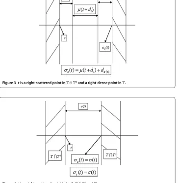
Figure 3 tis a right-scattered point inT∩Tsand a right-dense point inT.
Figure 4 tis a right-scattered point in bothT∩TsandT.
Then we can introduce the concept of almost periodic time scales as follows.
Definition .([, ]) We sayTis an almost periodic time scale if for any giveε> , there exists a constantl(ε) > such that each interval of lengthl(ε) contains aτ(ε)∈ such that
dT,Tτ<ε,
i.e., for anyε> , the set
E{T,ε}=τ∈:dTτ,T<ε
According to Definition ., we obtain the following useful lemmas.
Lemma . LetTbe an almost periodic time scale.Ifτ,τ∈ε,then there existsξ∈
ˆ
(τ,τ+τ]such thatξ∈ε,where
ˆ
(τ,τ+τ] =
⎧ ⎨ ⎩
(τ,τ+τ], τ<τ+τ,
[τ+τ,τ), τ>τ+τ.
Proof From the condition of the lemma, we obtain
dT,Tτ+τ<dT,Tτ+dTτ,Tτ+τ< ε.
CaseI. Ifd(T,Tτ+τ) <ε, thenξ
=τ+τ, and we get the desired result.
CaseII. Let ε>d(T,Tτ+τ) >ε. Note (.), let
f(x) =dT,Tx, x∈(τ,τˆ+τ],
and notef(x) is continuous onR. Now, letF(x) =f(x) –ε, and we obtain
F(τ) =f(τ) –ε< , F(τ+τ) =f(τ+τ) –ε> ,
so, there exists someξ∈(τ,τˆ+τ) such thatF(ξ) = . From the continuity ofF, we see
that there exists someξ∈ ˆ(τ,ξ) such thatF(ξ) < ,i.e., f(ξ) <ε. This completes the
proof.
Remark . From Lemma ., we can see thatεis an infinite number set.
Lemma . For anyε> andτ∈ε,if t∈T∩Tτ,then there existsτ∈εwithτ>τ such that t∈T∩Tτ.
Proof From Lemma ., there existsξ>τsuch thatd(T,Tξ) <ε.
CaseI. If fort∈T∩Tτ, we havet∈T∩Tξ, and thenτ=ξ∈ε.
CaseII. If fort∈T∩Tτ, we havet∈/T∩Tξ, thent∈/Tξ and
dTτ,Tξ<dT,Tτ+dT,Tξ< ε. (.)
Then we denoteγ=inft∈Tξ|t–t|+ε, and we get
inf
t∈Tξ|t–t| ≤d
Tξ
,T<ε,
so we haveγ< ε. Therefore, by (.), we obtain
inf t∈Tτ
αiξ+γ–t<ε and inf
t∈Tτ
βiξ+γ–t<ε,
so
αiξ+γ–αiτ<ε and β ξ
and so we obtain
αξi +γ>αiτ–ε and β ξ
i +γ>βiτ–ε.
Hence,
dT,Tξ+γ=max
sup
i∈Z αi–
αξi +γ,sup
i∈Z βi–
βiξ +γ
≤max
sup i∈Z
αi–
ατ
i –ε,sup i∈Z
βi–
βτ
i –ε=d
T,Tτ<ε.
Hence, we haveξ+γ∈εandt∈T∩Tξ+γ. Hence, we can takeτ=ξ+γ>τ such
thatt∈T∩Tτ. This completes the proof.
Remark . From Lemma ., one see that ifτ∈εandt∈T∩Tτ, then the set{τ ∈ ε:t∈T∩Tτ}is an infinite number set.
Letμτ:Tτ→R+be the graininess function ofTτ, and we obtain
μτ(t+τ) = ⎧ ⎨ ⎩
μ(t), t+τ∈/T,
μ(t+τ), t+τ∈T. (.)
Thus, from (.), we can simplify Definition . as follows.
Definition . Letμ:T→R+be a graininess function ofT. We sayTis an almost
peri-odic time scale if for anyε> , the set
∗=τ∈:μ(t+τ) –μ(t)<ε,∀t∈T∩T–τ
is relatively dense in.
Definition .([, ]) LetTbe an almost periodic time scale,i.e.,Tsatisfies Defini-tion .. A funcDefini-tionf ∈C(T×D,En) is called an almost periodic function int∈T uni-formly forx∈Dif theε-translation set off
E{ε,f,S}=
τ∈ε:f(t+τ,x) –f(t,x)<ε, for all (t,x)∈
T∩T–τ×
S
is a relatively dense set inεfor allε>ε> and for each compact subsetSofD; that is,
for any givenε>ε> and each compact subsetSofD, there exists a constantl(ε,S) >
such that each interval of lengthl(ε,S) contains aτ(ε,S)∈E{ε,f,S}such that
f(t+τ,x) –f(t,x)<ε, for all (t,x)∈
T∩T–τ×
S.
Thisτ is called theε-translation number off andl(ε,S) is called the inclusion length of E{ε,f,S}.
(i) for allt∈T∩(∪Tε), there exists–τ∈
εsuch thatt∈T∩T–
τ. From
Remark ., we know that the set{–τ ∈ε:t∈T∩T–
τ}is an infinite number set.
(ii) d(T∩(∪Tε),T) <ε
.
(iii) According to (i) from Remark ., for allt∈T∩(∪Tε), there exists an infinite
number set¯ ⊂εsuch thatt+τ ∈T.
Definition .([, ]) LetTbe an almost periodic time scale and assume that{τi} ⊂T
satisfying the derived sequence{τij},i,j∈Z, is equipotentially almost periodic. We call a functionϕ∈PCrd(T,Rn) almost periodic if:
(i) for anyε> , there is a positive numberδ=δ(ε)such that if the pointstandt
belong to the same interval of continuity and|t–t|<δ, thenϕ(t) –ϕ(t)<ε; (ii) for anyε>ε> , there is a relative dense setofε-almost periods such that if
τ∈⊂ε, thenϕ(t+τ) –ϕ(t)<εfor allt∈T∩(∪T
ε)which satisfy the
condition|t–τi|>ε,i∈Z.
Remark . From Definition ., ifTis a periodic time scale, then one can take a peri-odicity set˜ ⊂ofT, such thatμs(t) =μ(t) for allt∈T∩Ts=T,s∈ ˜,dt=dσ(t)= . If Tis an almost periodic time scale from [], then one can take aε-translation number set ε⊂ofT, such that|μs(t) –μ(t)|<εfor allt∈T∩Ts,s∈ε,i.e., for all right-scattered
and right-dense pointst∈T∩Ts, one can obtaind
t,dσ(t)<ε.
According to Definition . and Remark ., we can introduce a concept ofε-equivalent impulsive functional dynamic equations on almost periodic time scales as follows.
Definition . LetTbe an almost periodic time scale. Consider the following impulsive functional dynamic equations with sub-derivativex–s(t) onT∩T–s:
⎧ ⎨ ⎩
x–s(t) =f(t,x
t), t∈T∩T–s,t=tk,k∈Z,
x(tk) =Ik(x(tk)), t=tk,k∈Z,
(.)
where –s∈,xt(s) =x(t+s). We say the functional dynamic equations
⎧ ⎨ ⎩
x(t) =f(t,x
t), t∈T∩T–s,t=tk,k∈Z,
x(tk) =Ik(x(tk)), t=tk,k∈Z,
(.)
areε-equivalent impulsive functional dynamic equations for (.) if –s∈ε⊂. Note
that (.) can also be written as
⎧ ⎨ ⎩
x(t) =f(t,x
t), t=tk,k∈Z,
x(tk) =Ik(x(tk)), t=tk,k∈Z,
(.)
Remark . LetTbe an almost periodic time scale. According to Theorem . and Re-mark . from [], one can observe that we say the dynamic equations
⎧ ⎨ ⎩
x(t) =f(t,x
t), t∈T,t=tk,k∈Z,
x(tk) =Ik(x(tk)), t=tk,k∈Z,
have an almost periodic solution on the almost periodic time scaleTif (.) has an almost periodic solution onT∩T–sfor any –s∈
ε.
Remark . According to Theorems . and . from [], for (.), if we letxt(τ(t)) =
x(t–τ(t)),τ:T→ε, then it becomes ⎧
⎨ ⎩
x(t) =f(t,x(t–τ(t))), t=t k,k∈Z,
x(tk) =Ik(x(tk)), t=tk,k∈Z,
if we letxt(θ) = b
a x(t+θ)εθ, and then it becomes ⎧
⎨ ⎩
x(t) =f(t,b
a x(t+θ)εθ), t=tk,k∈Z,
x(tk) =Ik(x(tk)), t=tk,k∈Z.
Lemma .([]) Let A be a compact convex subset of a locally convex(linear topological) space and f be a continuous map of A into itself.Then f has a fixed point.
3 Characterizations of compact sets in a regulated functional space on time scales
In this section, we introduce some new definitions and establish new characterization results of compact sets in functional spaces on time scales which will play an important role in studying abstract discontinuous dynamic equations on time scales.
First, letδL+∞,δ+R∞: [T, +∞)T→R+∪ {}. Similar to [], we can extend the-gauge
for [a,b]Tto [T, +∞)T.
Definition . We sayδ+∞= (δ+∞
L ,δ+R∞) is a-gauge for [T, +∞)TprovidedδL+∞(t) >
on (T, +∞)TandδL+∞(T)≥,δR+∞(t) > on [T, +∞)TandδR+∞(t)≥μ(t) for allt∈
[T, +∞)T.
For a-gauge,δ+∞, we always assumeδ+∞
L (T)≥ (we will sometimes not even point
this out).
ForT∈Tand a Banach space (X, · ), let
G[T, +∞)T,X:=
x: [T, +∞)T→X;
lim s→t+x(s) =x
t+and lim s→t–x(s) =x
t–exist and are finite,
s,t< +∞and sup t∈[T,+∞)T
x(t)< +∞
.
Lemma . (G([T, +∞)T,X), · ∞)is a Banach space.
Proof Let{xn}be an arbitrary Cauchy sequence inG,i.e., for anyε> , there existsNsuch
thatn,m>Nimplies
xn(t) –xm(t)<ε for allt∈[T, +∞)T. (.)
SinceXis a Banach space, for eacht∈[T, +∞)T,{xn(t)} ⊂Xis a Cauchy sequence so
xn(t)→x(t). Hence, letm→+∞in (.), and we have
xn(t) –x(t)<ε for allt∈[T, +∞)T.
Furthermore, since{xn} ⊂G, for anyε> andt∈[T, +∞)T, there existsδ> ,t∈(t– δ+L∞(t),t)Twith
xn(t) –xn
t+<ε.
Hence, we obtain
x(t) –xt+≤x(t) –xn(t)+xn(t) –xn
t++xn
t+–xt+≤ε. (.)
Similarly, fort∈(t,t+δ+R∞(t))T, we also obtain
x(t) –xt–≤x(t) –xn(t)+xn(t) –xn
t–+xn
t––xt–≤ε. (.)
Therefore, from (.) and (.), we obtainx∈G. Hence,Gis a Banach space.
In the following, we will introduce the definition of a partitionP for [T, +∞)T.
Definition . A partitionPfor [T, +∞)Tis a division of [T, +∞)Tdenoted by P=T=tP ≤η≤tP≤ · · · ≤tnP–≤ηn≤tnP≤ · · ·<· · ·
withtPi >tiP–fori= , , . . . andti,ηi∈T. We call the pointsηitag points and the pointsti
end points.
Definition . Ifδ+∞is a-gauge for [T, +∞)T, then we say a partitionP isδ+∞-fine if
ηi–δL+∞(ηi)≤tiP–<tiP≤ηi+δR+∞(ηi)
fori= , , . . . .
Remark . From Definition ., one can observe that if a partitionP isδ+∞-fine for
[T, +∞)T, then for any closed interval [a,b]T⊂[T, +∞)T, there must exist aδ-fine
Definition . A setA⊂G([T, +∞)T,X) is called uniformly equi-regulated, if it has the
following property: for everyε> andt∈[T, +∞)T, there is aδ+∞= (δL+∞,δR+∞) such
that
(a) Ifx∈A,t∈[T, +∞)Tandt–δL+∞(t) <t<t, thenx(t–) –x(t)<ε. (b) Ifx∈A,t∈[T, +∞)Tandt<t<t+δ+R∞(t), thenx(t+) –x(t)<ε.
From Definition ., we obtain the following theorem.
Theorem . A setA⊂G([T, +∞)T,X)is uniformly equi-regulated,if and only if,for
everyε> ,there is aδ+∞-fine partitionP:
T=tP <tP<tP <· · ·<tnP<· · ·<· · ·
such that
xt–x(t)≤ε, (.)
for every x∈Aand[t,t]T⊂(tjP–,tjP)T,j= , , . . . .
Proof Letε> be given and let
D=ξ;ξ∈(T, +∞)T
such that there is a partitionP:
T=tP <tP<· · ·<tkP=ξ
for which (.) holds withj= , , . . . ,k.
(i) IfA⊂G([T, +∞)T,X) is uniformly equi-regulated, then there is aδR+∞(T) > such
that
x(t) –xT+<ε ,
for everyx∈Aandt∈(T,T+δR+∞(T))T. Denoteξ=T+δR+∞(T),T=tP <tP =ξ.
Thus, for [t,t]T⊂(T,ξ)Tandx∈A, the inequalities
x(t) –xt≤x(t) –xT++xt–xT+≤ε,
holds and we haveξ∈D.
Letξ>ξ>T. Sincex∈A, then there is aδL+∞(ξ) such that
xξ––x(t)<ε
for everyx∈Aandt∈(ξ–δL+∞(ξ),ξ)T∩[T, +∞)T.
Letξ˜∈(ξ–δL(ξ),ξ)Tand a partitionT=tP<tP<tP<· · ·<tkP=ξ˜be such that (.)
holds withj= , , . . . ,k. DenotetkP+=ξ. Then for [t,t]T⊂(tkP,tkP+)Tandx∈A, we have
which impliesξ∈D. Thus we use the same argument as before to find thatξi∈(ξi–, +∞)T
such thatξi∈D,i= , , . . . . Henceξ∞=supD= +∞and we are finished.
(ii) Reciprocally, for any givenε> , there is aδ+∞-fine partitionP:T=tP<tP <tP<
· · ·<tPk <· · ·<· · · such that
x(t) –xt≤ε, (.)
for everyx∈Aand [t,t]T⊂(tPj–,tPj )T,j= , , . . . .
Letηjbe a tag of (tj–,tj)T. Since this partition isδ+∞-fine, we have (tPj–,tjP)T⊂(ηj–
δ+L∞(ηj),ηj+δR+∞(ηj))T. Therefore, the inequality (.) holds, fort,t∈(ηj–δL+∞(ηj),ηj+
δ+R∞(ηj))T. Takingt=ηj–andt∈(ηj–δL+∞(ηj),ηj]T, then the inequality (.) remains true.
Also, ift=ηj+andt∈[ηj,ηj+δ+R∞(ηj))T, the inequality (.) is fulfilled. Then, from
Defi-nition ., it follows thatAis uniformly equi-regulated. This completes the proof.
Definition . LetA⊂G([T, +∞)T,X). We sayAis uniformly Cauchy if for anyε> ,
there existT∈(T, +∞)Tand aδ+∞= (δL+∞,δR+∞)-fine partitionP:
tP=T<tP <tP<· · ·<tnP<· · ·<· · ·
such that:
(a) Ifx∈A,t,t∈[T, +∞)Tandt–δL+∞(t) <t<t, thenx(t–) –x(t)<ε. (b) Ifx∈A,t,t∈[T, +∞)Tandt<t<t+δ+R∞(t), thenx(t+) –x(t)<ε. (c) Ifx∈A,t∈[a,b]T⊂(tjP–,tPj )T,t∈[a,b]T⊂(tiP–,tPi )T,i,j= , , . . ., then
x(t) –x(t)<ε.
Remark . From Definition ., one can observe that ifA⊂G([T, +∞)T,X) is
uni-formly Cauchy, then there existsT∈(T, +∞)Tsuch thatAis uniformly equi-regulated on [T, +∞)T.
Theorem . Assume that a set A⊂G([T, +∞)T,X)is uniformly equi-regulated and uniformly Cauchy,and for any t∈[T, +∞)T,there is a numberβtsuch that,for x∈A,
x(t) –xt–≤βt, x
t+–x(t)≤βt, t∈[T, +∞)T. (.)
Then there is a constant K > such thatx(t) –x(T) ≤K, for every x∈A and t∈
[T, +∞)T.
Proof SinceAis uniformly Cauchy, according to Definition ., there existsT∈(T, +∞)T
such that
x(t) –x(T)< , t∈[T, +∞)T. (.)
LetCbe the set of allτ∈(T,T]Tsuch that there existsKτ > such that
x(t) –x(T)≤Kτ,
SinceAis uniformly equi-regulated, there is aδ+R∞(T) such that
x(t) –xT+≤,
for everyx∈Aandt∈(T,T+δ+R∞(t)]T. This fact together with the hypothesis implies
that
x(t) –x(T)≤x(t) –x
T++xT+–x(T)≤ +βT:=KT+δ+∞,
for everyt∈(T,T+δR(T)]Tandx∈A. Hence, (T,T+δR(T)]T⊂C.
Denoteτ=supC. As a consequence of the uniformly equi-regulatedness ofA, there is
aδL+∞(τ) > such thatx(t) –x(τ–) ≤ forx∈Aandt∈[τ–δL+∞(τ),τ)T.
Letτ∈C∩[τ–δL+∞(τ),τ)T. Then
x(t) –x(T)≤x(t) –x
τ–+xτ––x(τ)+x(τ) –x(T)≤ + +Kτ= +Kτ,
for everyx∈Aandt∈(τ,τ)T. Also,
x
τ––x(T)≤x
τ––x(τ)+x(τ) –x(T)≤ +Kτ.
These inequalities and this hypothesis imply that
x(τ) –x(T)≤x(τ) –x
τ–+xτ––x(T)≤βτ+ +Kτ. (.)
Thusτ∈C, whereKτ=βτ+ +Kτ.
Ifτ<T, then, sinceAis uniformly equi-regulated, there is aδR+∞(τ) > such that
x(t) –xτ+≤, for anyx∈Aandt∈τ,τ+δR(τ)
T,
which implies
x(t) –x(T)≤x(t) –x
τ++xτ+–x(τ)+x(τ) –x(T)
≤ +βτ+Kτ=Kτ+δR+∞(τ),
fort∈(τ,τ+δ+R∞(τ)]Tandx∈A. Thusτ+δR+∞(τ)∈C, which contradicts the fact that τ=supC. Therefore,τ=T. Hence, by (.), we have
x(T) –x(T)≤Kτ.
Combining with (.), we have
x(t) –x(T)≤x(t) –x(T)+x(T) –x(T)≤ +Kτ,
fort∈(T, +∞)T. Then we can get the desired result.
Theorem . Let A ⊂ G([T, +∞)T,X) be uniformly equi-regulated and uniformly
Similarly, from (.) and (.), we also obtain
so we obtain
and, in this case, we have
ort∈(tP
Similarly, from (.), we also obtain
xnk(t) –xnq(t)≤xnk(t) –xnq
a convergent subsequence which means thatAis a relatively compact set. The proof is
complete.
In the following, letX=Rn; we will give some sufficient conditions to guarantee that
A⊂G([T, +∞)T,Rn) is relatively compact.
Theorem . Let a setA⊂G([T, +∞)T,Rn).IfAis relatively compact in the sup-norm topology,then it is uniformly equi-regulated.IfAis uniformly equi-regulated and uniformly Cauchy,satisfying(.),thenAis relatively compact inG([T, +∞)T,Rn).
Proof A subsetA of a Banach spaceX is relatively compact if and only if it is totally bounded, i.e., for every ε> , there is a finite ε-net F for A, i.e., such a subset F =
(i) Assume thatAis relatively compact. Then it is bounded by a constantC, and evidently (.) is satisfied withβt= Cfor everyt∈[T, +∞)T.
Lett∈[T, +∞)Tandεbe given. Let{x,x, . . . ,xk} ⊂G([T, +∞)T,Rn) be a finiteε /-net forA. For everyn= , , . . . ,k, there is aδ+n∞= (δL+∞,n,δR+∞,n) such that
xn(t) –xn
t+<ε
fort∈
t,t+δ+R∞,n(t)
T∩[T, +∞)T
and
xn
t––xn(t)<
ε
fort∈
t–δ+L∞,n(t),t
T∩[T, +∞)T.
Denoteδ+∞= (min≤n≤k(δL+∞,n(t)),min≤n≤k(δ+R∞,n(t))) = (δL+∞(t),δ+R∞(t)).
For arbitraryx∈A, we can findxn such thatx–xn∞ ≤ε/ for everyt∈(t,t+ δ+∞
R (t))T∩[T, +∞)T, and we have the inequality
x(t) –xt+≤x(t) –xn(t)+xn(t) –xn
t++xn
t+–xt+
≤x–xn∞+xn(t) –xn
t+<ε,
and similarly,|x(t–
) –x(t)|<εfort∈(t–δL+∞(t),t)T.
(ii) Assume thatAis uniformly equi-regulated, (.) holds,i.e., there existsα˜> such that|x(T)| ≤ ˜αfor everyx∈A.
From Theorem ., there is K such that |x(t) –x(T)| ≤K for any x∈ Aand t ∈
[T, +∞)T. Hence,|x(t)| ≤ |x(t) +x(T)|+|x(T)| ≤K+α˜. If we denoteγ˜ =K+α˜, then
x ≤ ˜γ forx∈A. SinceAis uniformly bounded inRn,Ais a sequentially compact closed
set in Rn,i.e.,Ais relatively compact inRn. From Theorem ., one can obtainAis a
relatively compact set inG([T, +∞)T,Rn). This completes the proof.
Remark . IfA˜is uniformly bounded, equi-continuous and uniformly Cauchy, thenA˜⊂ A. Hence, one can observe that Lemma from [] is just a particular case of Theorem ..
Remark . Fora,b∈T, let
G
[a,b]T,X:=
x: [a,b]T→X;
lim s→t+x(s) =x
t+and lim s→t–x(s) =x
t–exist and are finite
,
and according to eachx∈G, we can construct the setG([a, +∞)T,X), satisfying, for each
˜
x∈G:
˜
x(t) =
⎧ ⎨ ⎩
x(t), t∈[a,b]T,
x(b–), t∈(b, +∞)
T.
One can immediately see thatGandGare topological homeomorphic,i.e., there exists
a homeomorphic mappingf :G→G such thatf(x) =x˜ andf–(x˜) =x. Since for any
setA⊂G, according to the construction of the setG, one can see thatf(A) is uniformly
compactness off(A) is decided by the uniformly equi-regulatedness off(A). However, for all t∈(b, +∞)T, obviously,f(A) is uniformly regulated. Thus the uniformly
equi-regulatedness off(A) on [a, +∞)Tis actually decided by the equi-regulatedness ofAon [a,b]T. Therefore, ifAis equi-regulated on [a,b]T, thenf(A)⊂Gis relatively compact, i.e.,Ais relatively compact inG.
From Theorem . and Remark ., we can obtain the following corollaries.
Corollary . Let X=Rn.A set A⊂G
is relatively compact if and only if it is equi-regulated and for every t∈[a,b]T,the set{x(t);x∈A}is bounded inRn.
Proof IfA⊂Gis relatively compact, thenAis totally bounded inRn, and then for every t∈[a,b]T,{x(t);x∈A}is bounded inRn. Moreover, by Remark ., there exists a
home-omorphic mappingf :G→Gsuch thatf(A)⊂Gis relatively compact, which means
thatf(A)⊂Gis equi-regulated on [a,b]Taccording to Theorem .. Sincefis continuous
and a one-to-one mapping,Ais equi-regulated on [a,b]T.
IfA⊂Gis equi-regulated and for everyt∈[a,b]T, the set{x(t);x∈A}is bounded in Rn, thenf(A)⊂G
is equi-regulated and for everyt∈[a, +∞)T, the set{f(x);f(x)∈f(A)}
is bounded inRn, according to Theorem ., f(A) is relatively compact inG
,i.e.,Ais
relatively compact inG. This completes the proof.
Corollary . LetA⊂Gbe equi-regulated,and for every t∈[a,b]T,let the set{x(t);x∈
A}be relatively compact in X.Then the setAis relatively compact inG([a,b]T,X).
Proof From the assumption of this corollary and Remark ., by Theorem ., we can see that the setf(A) is relatively compact inG([a, +∞)T,X),i.e., the setAis relatively
compact inG([a,b]T,X). This completes the proof.
Remark . In fact, if we letT=R, Corollaries . and . can include Corollary . from [] and Theorem . from [], respectively.
Similarly, forT¯∈Tand a Banach space (X, · ), let
G(–∞,T¯]T,X
:=x: (–∞,T¯]T→X;
lim s→t+x(s) =x
t+and lim s→t–x(s) =x
t–exist and are finite,
s,t< +∞and sup t∈(–∞,T¯]T
x(t)< +∞
.
From Definition ., we can also introduce aδ–∞ and extend the-gauge for [a,b]
Tto
(–∞,T¯]T, and then we can repeat the same above discussion, and the following theorems
can also be obtained (we omit the proofs).
Theorem . Assume that a setA⊂G((–∞,T¯]T,X)is uniformly equi-regulated and uniformly Cauchy,and for any t∈(–∞,T¯]T,there is a numberβtsuch that,for x∈A,
x(t) –xt–≤βt, x
Then there is a constant K > such thatx(t) –x(T¯) ≤K, for every x∈A and t∈
(–∞,T¯]T.
Theorem . Let A ⊂ G((–∞,T¯]T,X) be uniformly equi-regulated and uniformly
Cauchy,for every t∈(–∞,T¯]T,let the set{x(t);x∈A}be relatively compact in X.Then the setAis relatively compact inG((–∞,T¯]T,X).
Theorem . Let a setA⊂G((–∞,T¯]T,Rn).IfAis relatively compact in the sup-norm topology,then it is uniformly equi-regulated.IfAis uniformly equi-regulated and uniformly Cauchy,satisfying(.),thenAis relatively compact inG((–∞,T¯]T,Rn).
For the more general case, for a Banach space (X, · ), let
G(–∞, +∞)T,X:=
x: (–∞, +∞)T→X;
lim s→t+x(s) =x
t+and lim s→t–x(s) =x
t–exist and are finite,
–∞<s,t< +∞and sup t∈(–∞,+∞)T
x(t)< +∞
.
From Definition ., we can also introduce aδ±∞ and extend the-gauge for [a,b]Tto
(–∞, +∞)T, since for anyT>T¯, (–∞, +∞)T= (–∞,T¯]T∪[T¯,T]T∪[T, +∞)T, and
then we can repeat the above discussion, and the above similar theorems can also be ob-tained (we omit these similar statements here).
Let
G[T, +∞)T:=
x;x∈PCrd
[T, +∞)T,Rn
and sup
t∈[T,+∞)T
x(t)< +∞
,
wherePCrd([T, +∞)T,Rn) is the set formed by all rd-piecewise continuous functions (one
can consult Definition . from []). EndowGwith the normx=supt∈[T,+∞)T|x(t)|,
and note (G, · ) is a Banach space.
Next, we will establish some theorems to guarantee thatA⊂G([T, +∞)T,Rn) is
uni-formly Cauchy and uniuni-formly equi-regulated.
Now, we give a new definition called ‘equi-absolutely continuity’ for the function set A⊂G, which will be used in the following lemma’s proof.
Definition . LetA⊂G. We sayAis equi-absolutely continuous if for anyf ∈Aand ε> , there existsδ> , such that for any finite mutually disjoint open interval (xi,yi)T⊂
[T, +∞)T(i= , , . . . ,n)
n
i=
(yi–xi) <δ
implies
n
i=
Lemma . LetA⊂G([T, +∞)T,Rn)be uniformly bounded and
Z =t∈[T, +∞)T:x is not-differentiable at t
andμ(Z) = for all x∈A,i.e.,x is-differentiable at[T, +∞)T\Z and there exists M> such that|x(t)| ≤M for all x∈A.ThenAis uniformly equi-regulated,and for any
ε> ,there exists T> such that,for any x∈A,the following is fulfilled:
[T,+∞)T\Z
x(s)s≤ε.
Proof From the condition of the theorem, sincexis-differentiable at [T, +∞)T\Z and
there existsM> such that|x(t)| ≤M, according to Corollary . from [], we can
obtain for allt∈[T, +∞)T\Z,x(t) satisfies the Lipschitz condition
x(t) –x(t)≤M|t–t|, ∀t,t∈[T, +∞)T\Z.
So for eachN∈Z+, we can obtain
N
j=
tj–tj< ε M,
tj,tjT⊂[T, +∞)T, (.)
which implies
N
j=
xtj–xtj<M
N
j=
tj–tj<ε, (.)
i.e.,Ais equi-absolutely continuous on [T, +∞)T\Z. Hence, from (.) and (.), for
allt∈[T, +∞)T\Z,Ais uniformly equi-regulated. For allt∈Z, sinceμ(Z) = , from
(.) and (.), we can takeδ+∞= (δ+∞
L ,δ+R∞) andδL,δR<Mε, so
x
t+–x(t)<
N
j=
x
tj–xtj<ε ift∈t,t+δR+∞(t)
T
and
xt––x(t)<
N
j=
xtj–xtj<ε ift∈t–δL+∞(t),t
T,
and thusAis uniformly equi-regulated on [T, +∞)T. According to Theorem ., for any
closed interval [aP,bP]T, there is aδ +∞
-fine partitionP:
aP:=T=t P
<tP<tP<· · ·<tPN:=bP
such that
i.e.,tPi
In the following, we will give the following useful corollaries.
Corollary . LetA⊂G([T, +∞)T,Rn)be uniformly bounded and
Z =t∈[T, +∞)T:x is not-differentiable at t
andμ(Z) = for all x∈A,and there exists M> such that|x(t)| ≤M for all x∈A.
ThenAis relatively compact inG.
Proof According to Theorem .,Ais uniformly equi-regulated, uniformly Cauchy. Fur-ther, sinceAis uniformly bounded, so it satisfies (.), by Theorem ., we get the desired
Let
BC[T, +∞)T:=
x∈BC[T, +∞)T,Rnand sup
t∈[T,+∞)T
x(t)<∞
,
where BC([T, +∞)T,Rn) denotes the set of all bounded continuous functions on [T,
+∞)T. Then we can obtain the following corollary.
Corollary . Let A⊂BC[T, +∞)T be uniformly bounded and for all x∈A, x is -differentiable and there exists M> such that|x(t)|<M.ThenAis relatively compact in
BC.
Proof Since x is -differentiable on [T, +∞)T, A is equi-absolutely continuous on [T, +∞)T, for anyt,t∈[T, +∞)T, we can obtain
x(t) –x(t)=
tt
x(s)s≤ sup t∈[T,+∞)T
x(t)< M,
which means that
t+∞
x(s)s< M
, Mis some constant.
Thus, for anyε> , there existsT> , and we havet>t>Timplies
xt–xt=
t
t
x(s)s<ε,
i.e.,Ais uniformly Cauchy. According to Theorem .,Ais relatively dense inBC. This
completes the proof.
Remark . Note that if for allx∈A⊂BC,xhas uniformly bounded-derivatives, then one can see thatAis equi-absolutely continuous, which will lead to thatAis uniformly Cauchy. Hence, the uniformly boundedness ofAand the uniformly boundedness of -derivatives functions ofAcan guaranteeAis relatively compact.
4 Existence of solutions for impulsive functional dynamic equations
In this section, we introduce some new definitions and give some new methods to obtain some sufficient conditions for the existence of solutions for a class ofε-equivalent impul-sive functional dynamic equations on almost periodic time scales. We always assume that
supT= +∞andinfT= –∞.
Definition . For arbitrary functionsx,y:T→Rn, we define the function [x(·),y(·)] μ:
T→Rto be the number (provided it exists) with the property that, for any givenε> , there exists a neighborhoodUoft(i.e.,U= (t–δ,t+δ)Tfor someδ> ) such that
Remark . In Definition ., iftis a right-dense point,μ(t) = , then one can obtain
x(t),y(t)=lim s→t
|x(t) +|t–s|y(t)|–|x(t)|
|t–s| , (.)
lets–t=h→+, and (.) can be written as
x(t),y(t)= lim h→+
|x(t) +hy(t)|–|x(t)|
h . (.)
Iftis a right-scattered point,μ(t) > , then one can get
x(t),y(t)μ=|x(t) +μ(t)y(t)|–|x(t)| μ(t) .
In the following, we will consider the following impulsive system:
⎧ ⎨ ⎩
x(t) =A(t,x) +g(t), t=t k,
x(tk) =˜Ik(x(tk)), t=tk,k∈Z,
(.)
whereA∈PCrd(T×Rn,Rn),g∈PCrd(T,Rn),˜Ik∈C(Rn,Rn).
Next, we will give the following theorem to guarantee that (.) has a unique global solution.
Theorem . LetTbe a time scale with the bounded graininess functionμ.In the system (.),if for anyε> ,there exists a neighborhood U of t such that
˜
dx(t) +σ(t) –sA(t,x) +g(t),Br()
<εσ(t) –s, s∈U, (.)
for all(t,x)∈(tk–,tk)T×Br(),k∈Z,whered˜(z,Br())denotes the distance from z to Br()
and Br() ={x∈PCrd(T,Rn) :x ≤r,r is a constant}.Then for each tn∈T(n∈N),the Cauchy problem with the initial value x(tn
) =unfor(.)has a unique global solution x(t)
onTsuch that x∈Br()for all t∈T.
Proof Consider the following form of (.):
⎧ ⎨ ⎩
x(t) =Ax˜ (t) +A(t,x) –Ax˜ (t) +g(t), t=t k,
x(tk) =˜Ik(x(tk)), t=tk,k∈Z,
(.)
whereA˜ =A(t, ). From Theorem . from [], for anyt∈T, we can findk∈Z,tk–< t≤tk, fort∈[t,tk)T, there is a unique solution
x(t) =eA˜(t,t)x(t) +
t
t eA˜(t,s)
A(s,x) –Ax˜ (s) +g(s)s,
and by usingx(tk+) –x(t–
k) =˜Ik(x(tk)), we obtain
xtk+=eA˜(tk,t)x(t) + tk
t
eA˜(tk,s)
A(s,x) –Ax˜ (s) +g(s)s+˜Ik
x(tk)
and then we have
Hence, fort≥t, we know that (.) has a unique solution satisfying
x(t,x) =eA˜(t,t)x+
Therefore, (.) has a unique global solution un(t) onT. Furthermore, combining with
(.), for allt∈(tk–,tk)T,k∈Z,i.e.,t=tk, (.) can be changed into the following:
˜
dx(t) +σ(t) –sx(t),Br()
<εσ(t) –s. (.)
Case . Iftis a right-dense point, from (.), we obtain
˜
Case . Iftis a right-scattered point, from (.), we get
Thus, ifρ(t) <t, that is,ρ(t) is a right-scattered point, we haveσ(ρ(t)) =t, by (.), one has
˜
dx(t),Br()
=d˜xσρ(t),Br()
<ε.
Ifρ(t) =t, that is,tis a left-dense point, so there must exist a right-dense points, for any ε> , there exists aδ+L∞> such thats∈(t–δL+∞(t),t)Timplies
˜
dx(s),x(t)<ε.
Hence, by (.), we can easily get
˜
dx(t),Br()
<d˜x(t),x(s)+d˜x(s),Br()
<ε+ε= ε, t=tk,k∈Z.
For the impulsive pointstk,k∈Z, since (tk–δL+∞(tk),tk)T⊂(t–δ+L∞(t),t+δR+∞(t))T,
where|t–tk|<min{δL+∞(t),δR+∞(t)}, then
˜
dx(tk),Br()
<d˜x(tk),x
tk–+d˜xtk–,x(s)+d˜x(s),Br()
<ε+ε+ε= ε,
wheres∈(tk–δ+L∞(tk),tk)T⊂(t–δL+∞(t),t+δR+∞(t))T,k∈Z. This completes the proof.
Lemma . Let functions x,y,z : T→ Rn. Then for any a ∈R+ ∪ {}, the function
[x(·),y(·)]μhas the following properties:
(i) |[x(t),y(t)]aμ| ≤ |y(t)|.
(ii) [x(t),y(t) +z(t)]aμ≤[x(t),y(t)]aμ+ [x(t),z(t)]aμ.
(iii) Letu(t)be a function from an intervalJ⊂TintoRnsuch thatu(t
)exists for an
interior pointtofJ.ThenD+|u(t)|exists and
D+u(t)
=u(t),u(t)
μ,
whereD+|u(t)|denotes the right derivative of|u(t)|att.Further,for any a∈R+∪ {},we have[u(t
),u(t)]μ≤D+|u(t)|.
Proof Ifa= , thenaμ= , from Remark ., the results (i)-(iii) are obvious. Ifa∈R+, we can conclude the following:
(i) In fact, iftis a right-dense point, by (.), the result is obvious. Lettbe a right-scattered point, then
x(t),y(t)aμ=|x(t) +aμ(t)y(t)|–|x(t)| aμ(t)
≤|x(t) +aμ(t)y(t) –x(t)|
aμ(t)
(ii) Iftis a right-dense point, by (.), the result is obvious. Lettbe a right-scattered point, then
x(t),y(t) +z(t)aμ = |x(t) +aμ(t)(y(t) +z(t))|–|x(t)| aμ(t)
= |
x(t) +aμ(t)y(t) +
x(t) +aμ(t)z(t)|–|x(t)| aμ(t)
≤
|x(t) + aμ(t)y(t)|+
|x(t) + aμ(t)z(t)|–|x(t)| aμ(t)
= (|x(t) + aμ(t)y(t)|–|x(t)|) + (|x(t) + aμ(t)z(t)|–|x(t)|) aμ(t)
= |x(t) + aμ(t)y(t)|–|x(t)|
aμ(t) +
|x(t) + aμ(t)z(t)|–|x(t)| aμ(t)
=x(t),y(t)aμ+x(t),z(t)aμ.
(iii) Iftis a right-dense point, by (.), the result is obvious. Lettbe a right-scattered point, then
u(t),u(t)
μ=
|u(t) +μ(t)u(t)|–|u(t)| μ(t)
=|u(t) +μ(t)
u(σ(t))–u(t)
μ(t) |–|u(t)| μ(t)
=|u(σ(t))|–|u(t)| μ(t)
=D+u(t)
.
Further, fora∈R+, we can obtain
u(t),u(t)
aμ =
|u(t) +aμ(t)u(t)|–|u(t)| aμ(t)
= |u(t) +aμ(t)
u(σ(t))–u(t)
μ(t) |–|u(t)| aμ(t)
= |au(σ(t)) –au(t) +u(t)|–|u(t)| aμ(t)
≤ |au(σ(t)) –au(t) +u(t) –u(t)| aμ(t)
=D+u(t)
.
This completes the proof.
From Definition ., we obtain the following theorem, which guarantees that (.) has a unique global solution onT.
Theorem . Let A∈PCrd(T×Rn,Rn),g∈PCrd(T,Rn)be bounded,A(t, ) = for all
t∈Tand Ik() = ,be relatively dense inR.Suppose that there exist positive numbers
p>M> ,r> such that|g(t)| ≤M,p>Mr and
for t∈(tk–,tk),k∈Z, –p∈R+,a∈R+∪ {},|x(t)| ≤r,|y(t)| ≤r,and
the Cauchy problem for (.) with the initial valuex(tn
) =u.
For eachx∈Rnwith|x|=r, fort∈(t
k–,tk)T,k∈Z, (.) and (ii) in Lemma . imply
x,A(t,x) +g(t)μ≤x,A(t,x)μ+g(t)≤–p|x|+M= –pr+M< .
So for anyε> , there exists a neighborhood ofUsuch that
x+σ(t) –sA(t,x) +g(t)–|x|<x+σ(t) –sA(t,x) +g(t)–|x|
and (iii) from Lemma . imply