Earth Planets Space,61, 357–371, 2009
Estimation of scan-gap limits on phase delay connections in Delta VLBI
observations based on the phase structure function
at a short time period
Tetsuro Kondo1,2, Thomas Hobiger1,3, Mamoru Sekido1, Ryuichi Ichikawa1,
Yasuhiro Koyama1, and Hiroshi Takaba4
1Kashima Space Research Center, National Institute of Information and Communications Technology, 893-1 Hirai, Kashima, Ibaraki 314-8501, Japan
2Ajou University, San 5, Woncheon-dong, Yeongtong-gu, Suwon 442-749, Korea 3Institute of Geodesy and Geophysics, Vienna University of Technology,
Gusshausstrasse 27-29 E128, A-1040 Wien, Austria 4Gifu University, 1-1 Yanagido, Gifu-shi, Gifu 501-1193, Japan
(Received August 21, 2007; Revised August 28, 2008; Accepted October 15, 2008; Online published March 3, 2009)
The maximum scan-gap length which connects phase delays from scan to scan over a gap is an important issue in Delta Very Long Baseline Interferometry (D-VLBI), and it is affected by delay fluctuations caused by the wet troposphere. It has recently become possible to obtain near real-time fringe phases by using an e-VLBI technique that realizes real-time VLBI by connecting stations through high-speed Internet. Such real-time VLBI raises the possibility of dynamic D-VLBI scheduling, which changes scan and gap length dynamically according to the weather condition of the date. We have investigated this possibility by using phase structure functions obtained from continuous VLBI observations at S- and X-bands for 1–2 h at the Kashima, Gifu, and Koganei stations (not real-time ones). Five VLBI sessions were conducted during this study between March and July 2006 under different weather conditions. At first a simple method was developed to evaluate phase connectivity from a phase structure function. A model was also proposed to estimate a phase-structure function at longer time periods from a short time period. Finally, an available gap length was estimated using the model. Our results show that it is possible to estimate an available scan gap length by using a structure function at a time period of 10 s. This suggests that it is possible to control scan length and gap length dynamically in order to achieve the best performance of D-VLBI observations.
Key words:Delta VLBI, phase structure function, phase connection.
1.
Introduction
Delta (or differential) Very Long Baseline Interferom-etry (D-VLBI) is a technique which accurately measures the angular separation between two nearby celestial radio sources by observing each source alternately. Common error sources, such as those introduced by receiving sys-tems, clocks, propagating media, and station locations, are nearly cancelled by differences in observed delays between sources. If the position of one source is known well, the po-sition of the other source can be measured through the well-known source position. Since the late 1970’s (e.g., Brunn
et al., 1978; Christensenet al., 1980), this technique has been used for the navigation of deep-space spacecrafts (SC) by alternately observing SC and a nearby extragalactic ra-dio source (EGRS). Since an antenna tracks an SC and an EGRS alternately, gaps in each data stream are inevitable. Consequently, the fringe phase of each data segment (scan) has an ambiguity with multiples of 2π. When observations are carried out at a narrow band width, such as in the case of
Copyright cThe Society of Geomagnetism and Earth, Planetary and Space Sci-ences (SGEPSS); The Seismological Society of Japan; The Volcanological Society of Japan; The Geodetic Society of Japan; The Japanese Society for Planetary Sci-ences; TERRAPUB.
receiving carrier signals emitted from an SC, it is important to connect the fringe phases of corresponding scans without an ambiguity of 2π multiples in order to improve the accu-racy of the measurements. Wu (1979) developed a scheme to connect fringe phases among consecutive scans based on the iterative adjustment of integer ambiguity numbers. He applied the method to D-VLBI observations of Voyager 1 and OJ287 and concluded that when there was no sizable localized phase fluctuation (mainly due to the atmospheric disturbances), the scheme connected VLBI fringe phases faultlessly. Both scan and gap lengths were about 5 min in his study. A limitation in the gap lengths was not men-tioned in his paper. However, as long as narrow-band carrier signals from an SC are received in D-VLBI, the phase am-biguity problem is inevitable. Hence, this problem has led to the development of a new technique aimed at abtaining an unambiguous delay from SC measurements by adopting bandwidth synthesis (Rogers, 1970) to a number of tones emitted from an SC spanned over several tens of mega-hertz, which depends on the design of the SC’s telemetry system. Such unambiguous delay is called differential one-way range (DOR), and D-VLBI that has adopted DOR is termed DOR (e.g., Thornton and Border, 2003). Using an error budget analysis of theDOR, Border and Koukos
358 T. KONDOet al.: PHASE DELAY CONNECTION IN VLBI Table 1. Session summary.
Date Time Source Stations Weather Elevation at middle (deg)
March 16, 2006 12:00–13:00 UT 3C273B Kashima 34m rainy 36.2
Gifu 11 m rainy 33.6
April 19, 2006 13:00–15:00 UT 3C273B Kashima 34 m cloudy 54.6
Gifu 11 m cloudy 55.9
May 10, 2006 13:00–15:00 UT 3C273B Kashima 34 m cloudy 45.3
Gifu 11 m rainy 47.9
May 11, 2006 13:00–15:00 UT 3C273B Kashima 34 m cloudy 44.7
Gifu 11 m fair 47.3
July 21, 2006 15:00–17:00 UT 3C454.3
Kashima 34 m cloudy 61.2
Gifu 11 m rainy 58.8
Koganei 11 m light rain 60.5
136˚ 137˚ 138˚ 139˚ 140˚ 141˚ 142˚ 34˚
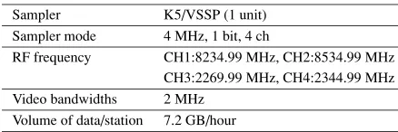
RF frequency CH1:8234.99 MHz, CH2:8534.99 MHz CH3:2269.99 MHz, CH4:2344.99 MHz Video bandwidths 2 MHz
Volume of data/station 7.2 GB/hour
(1994) demonstrated that the overallDOR measurement accuracy is about 0.23 ns, which corresponds to an angular position accuracy of about 9 nrad (nanoradian) for a pro-jected baseline length of 8,000 km.
Recently, the position measurements of NOZOMI, which is a Japanese Mars explorer (Yamamoto and Tsuruda, 1998), and HAYABUSA, which is a Japanese mission for near-Earth-asteroid sample return (Fujiwara et al., 1999), were carried out in Japan by means of D-VLBI (Ichikawa
et al., 2004; Sekido et al., 2004; Ichikawa et al., 2006). The D-VLBI technique is also used for studying the lu-nar gravity field in the Japanese lulu-nar explorer SELENE (KAGUYA) (Konoet al., 2003; Kikuchiet al., 2004). In the SELENE experiment, radio signals dedicated to D-VLBI-likeDOR are emitted from an SC. However in the NO-ZOMI and HAYABUSA experiments, narrow-band signals emitted from an SC were observed in order to investigate the possibility of the orbit determination without the use
of signals dedicated to theDOR, and the connection of fringe phases among consecutive scans was again recog-nized as an important parameter to achieve a delay mea-surement accuracy equal to that of theDOR (0.23 ns). Because the fluctuated fringe phases, mainly due to the wet troposphere, limit the gap length over which fringe phases can be connected, the antenna switching time should be less than this time span. Therefore, the maximum limit of the gap length as well as source strength are a critical parame-ters for promoting D-VLBI successfully. A gap length limit should depend on weather condition and, therefore, vary not only spatially but also temporally. It is therefore im-portant to dynamically determine the limit of the gap length for achieving the best performance of D-VLBI observation under any weather conditions. Statistical characteristics of atmospheric phase fluctuations have been investigated us-ing radio interferometry, includus-ing VLBI (e.g., Rogers and Moran, 1981; Rogers et al., 1984; Kasuga et al., 1986; Treuhaft and Lanyi, 1987; Liuet al., 2005). Beasley and Conway (1995) predicted a critical switching time based on their analysis of structure functions to 160–440 s at a fre-quency of 8.4 GHz and 25–30 s at 43 GHz at zenith angles less than 60◦. A switching time of 300 s is therefore rec-ommended for phase referencing observation of the VLA and VLBA for frequencies 1.4–8.4 GHz under typical at-mospheric conditions (Wrobelet al., 2000). The e-VLBI technique is developing rapidly (e.g., Koyamaet al., 2006; Whitney and Ruszczyk, 2006), enabling scientists to ob-tain near real-time fringe phases. If we know the gap limit using such a real-time observation, we could control scan length and gap length (i.e., switching time) dynamically in order to achieve the best performance of D-VLBI obser-vations. To this end, we have investigated the possibility of dynamic scheduling of D-VLBI observations using data obtained from a series of VLBI sessions with the aim of investigating fringe phase fluctuations.
T. KONDOet al.: PHASE DELAY CONNECTION IN VLBI 359
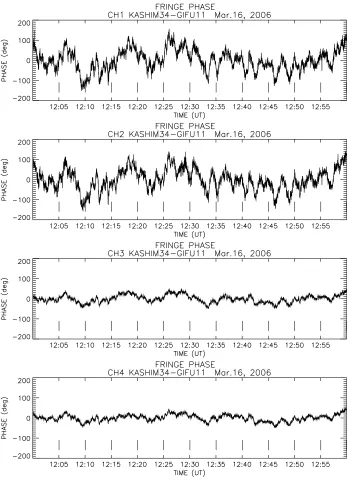
Fig. 2. Examples of fringe phase data after the connection of sub-observations and the removal of linear and second order trends for observations on March 16, 2006. Boundaries of sub-observations are displayed by short vertical bars, so that time between bars denotes 5 min. Frequencies from top to bottom are 8234.99 MHz, 8534.99 MHz, 2269.99 MHz, and 2344.99 MHz, respectively.
actual linear fitting of fringe phases, and the validity of the proposed method is discussed.
2.
Observations and Correlation Processing
Five VLBI sessions were conducted to investigate the re-lations between scan length and gap length between March and July, 2006, as summarized in Table 1. The Kashima 34-m antenna and Gifu 11-m antenna were used in all ses-sions, but the Koganei 11-m antenna was used only in the last session. At all stations, a hydrogen maser oscillator was used to provide the system reference signals. The locations of stations are shown in Fig. 1.
A strong source (either 3C273B or 3C454.3) was ob-served at each session for 1 or 2 h continuously using four channels of geodetic-VLBI backend outputs. The RF
fre-quencies were set to 8234.99 and 8584.99 MHz in X-band and 2269.99 and 2344.99 MHz in S-band, and the video bandwidth was set to 2 MHz. Four-channel video signals were converted into 1-bit digital signals at a sampling fre-quency of 4 MHz using the K5/VSSP system (Kondoet al., 2003), which results in a data rate of 16 Mbps (Mega bits per second) per station. Sampled data were stored on a hard disk in real time. Details of the condition of data acquisition are summarized in Table 2.
360 T. KONDOet al.: PHASE DELAY CONNECTION IN VLBI
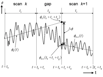
Fig. 3. Principle of the phase connection over a scan gap. Phases can be connected without ambiguities in case of|φ|<180◦.
However it is easy to connect data over such a small gap, so that we can regard a series of sub-observations as one continuous observation for our analyses described later.
After all observations of a session were finished, the data of Gifu and Koganei were transferred to Kashima through the Internet. Correlation processing was carried out using a software correlator dedicated to the processing of geodetic VLBI data (Kondoet al., 2004). The software correlator can process data on each scan basis with a flexible com-bination of the parameters lag lengths and unit integration period. We processed the data in the same fashion as that of normal-geodetic VLBI, i.e., 32 lags and a unit integration period of 1 s. A physical model used for the calculation of a-priori delay and delay rate was identical to that used for geodetic VLBI to ensure that the model has sufficient ac-curacy for our study. A-priori delay and delay rates were calculated for each sub-observation. Discrepancies at the boundaries of sub-observations are kept less than 0.01 ns for delay and 2×10⁻¹⁴ s/s for delay rate, corresponding
to a fringe phase of 28.8◦ and a fringe rate of 0.00016 Hz at 8 GHz. After correlation processing, residual delay and delay rate are determined every sub-observation by a coarse search, which calculates a so-called coarse search function. This is a function of trial delay and delay rate to find out the residual delay and delay rate which maximize the am-plitude of the function (see, for example, Takahashiet al.
(2000) for details of this processing). Observed delay and delay rate at an epoch of each sub-observation are computed by adding these residuals to the a-priori values. Therefore, as long as the discrepancy in the a-priori values is small enough to keep coherency in a unit integration period, it will not affect the observed delay and delay rate. More-over, the model has sufficient accuracy to keep the position of correlation peak within a lag (0.25μs) during the en-tire session, i.e., 1–2 h. Figure 2 shows examples of fringe
phase data after sub-observation connection and removal of linear and second order trend for the observation on May 11, 2006. Boundaries of sub-observations are displayed by short vertical bars in the Fig. 2.
3.
Data Analysis
3.1 Estimation of available scan-gap length from a phase structure function
A simple method has been developed to evaluate an avail-able scan-gap length using a phase structure function. Fig-ure 3 shows the principle of phase connection between con-secutive scans (scan numbers are k and k+1, and scan length= ts) separated by a gap (length= tg). A phase at the starting time of scank+1 (i.e.,t=tk+ts+tg) is
esti-mated as an extrapolated phase using a linear fitting of data at scankspanningt=tktotk+ts.
The phase is then compared with a phase att =tk+ts+tg
estimated from a linear fitting in the scank+1.
If the difference between these phases is smaller than 180◦, phases are considered to be connected without am-biguities. Thus, the variance of these phase errors provides information on the connectivity of phases.
A line fitted to observed phaseφ(t)for scankis given by φk(t)=akt+bk (1)
wherek is an index to represent scan number, andak and bkare fitting coefficients for scank. Sinceφk(t)is a linear
fitted line toφ(t),
φ(t)=φk(t)+εk(t) (2)
whereεk(t)is a fitting residual att. An extrapolated phase
att =tk+ts+tgcan be expressed using Eq. (1) as
φk(tk+ts+tg)=ak(tk+ts+tg)+bk
T. KONDOet al.: PHASE DELAY CONNECTION IN VLBI 361
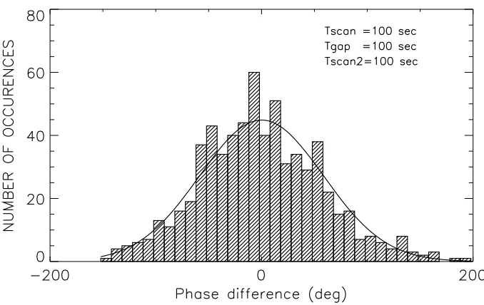
Fig. 4. An example histogram ofφfor the case of scan length=100 s and gap length=100 s for 8234.99 MHz data for the session on May 11, 2006. Standard deviation is 58.5◦.
Using Eq. (2), Eq. (3) can be rewritten as
φk(tk+ts+tg)=φ(tk+ts)−εk(tk+ts)+aktg. (4)
Using Eq. (2), we also obtain
φk+1(tk+ts+tg)=φ(tk+ts+tg)−εk+1(tk+ts+tg).
(5)
Hence using Eqs. (4) and (5), the difference between φk(tk+ts+tg)andφk+1(tk+ts+tg)is given as
φ=φk(tk+ts+tg)−φk+1(tk+ts+tg)
=[φ(tk+ts)−φ(tk+ts+tg)]+aktg
−[εk(tk+ts)−εk+1(tk+ts+tg)]. (6)
Therefore the variance can be expressed as
(φ)2 = [φ(t
where denotes the operation of averaging. Sinceak,εk,
andεk+1are thought to be independent stochastic variables,
the average of their cross-term will be small compared with other terms. Hence, we omit these cross terms and obtain
(φ)2 = [φ(t
The effect of cross terms will be discussed later.
Now, as the scan length is the same for scankandk+1,
ε2
kandε2k+1coincide with each other (=ε2). Moreover,
using a phase structure function defined as
σ2(τ)= [φ(t)−φ(t+τ)]2, (9)
we obtain
(φ)2 =σ2(tg)+t2
ga2k +2ε2. (10)
Statistical characteristics of fringe phase fluctuations usu-ally differ from a normal distribution on the time scale used in this study. However, we apply a fitting error based on a normal distribution variable to simplify the problem. The effect of this assumption will be discussed later. Henceεis given as
ε2 =1
4t
2
sσa2+σb2 (11)
whereσa andσb are estimation errors for parameteraand b. Hence, assumingak2 =σa2, we get
The second term of the right-hand side of Eq. (12) repre-sents a propagated phase error over a gap due to the error of the phase changing rate.
Regarding a linear fitting, we consider the simplest case, that is a line fitting using phases only att =tk andtk+ts
and assuming that the variance of their phase difference has an errorσ2
whereσ2(ts)is a phase structure function atts. The relation between a phase error due to thermal noise and signal-to-noise ratio (SNR) can be written as
σφ= 1
SNRu (14)
where SNRu is an SNR at a unit integration period at the
362 T. KONDOet al.: PHASE DELAY CONNECTION IN VLBI
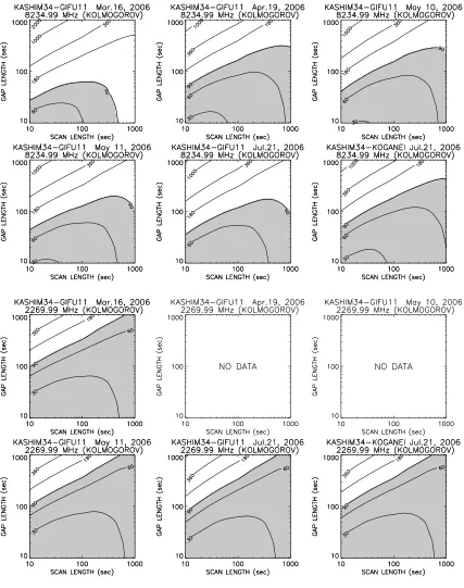
Fig. 5. Contour plots of standard deviations ofφon a scan and gap length plane obtained from phase structure functions for six baseline data from the five sessions carried out on March 16, April 19, May 20, May 21, and July 21, 2006, respectively. Upper six pannels are for 8234.99 MHz and lower six for 2269.99 MHz.
given as
σ2
b =
σ2
φ
ts =
1 (SNRu)2ts =
1
(SNR)2 (15)
whereSNRdenotes an SNR integrated over the whole scan length. Here, we assume that the only source of noise is thermal noise to simplify the problem. The effect of this assumption will be discussed later. Hence Eq. (12) can be
rewritten usingSNRas
(φ)2 =σ2(tg)+
1 2+
t2 g t2 s
σ2(ts)+ 2
(SNR)2. (16)
Thus, if a phase structure function and SNR are given, we can evaluate the phase error variance from Eq. (16). On the other hand,σφ can also be expressed by using a phase structure function as
σ2
φ =
1 2σ
T. KONDOet al.: PHASE DELAY CONNECTION IN VLBI 363
Fig. 6. Same as Fig. 5 but obtained from the actual linear fitting of phase data.
where tu is a unit integration period (1 s in this study). Applying this to Eq. (17), we get
(φ)2 =σ2(t g)+
1 2 +
tg2 t2 s
σ2(t s)+
1
tsσ 2(t
u). (18)
Equation (18) shows that we can evaluate the connectivity of fringe phases only from the phase structure function. In case of gap length=scan length, Eqs. (16) and (18) can be
simplified as follows
(φ)2 = 5
2σ
2(t s)+
2
(SNR)2 (19) = 5
2σ
2(ts)+1 tsσ
2(tu). (20)
If an SNR integrated over the span length is high enough, we can neglect the SNR term. The variance then becomes
(φ)2 = 5
2σ
364 T. KONDOet al.: PHASE DELAY CONNECTION IN VLBI
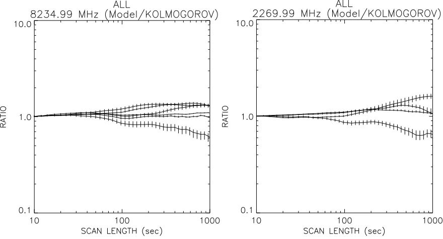
Fig. 7. Ratios of standard deviation of phase errors obtained from phase structure functions and those obtained from actual linear fitting for 8234.99 MHz (left panel) and for 2269.99 MHz (right panel). Averaged values over gap length between 10 and 1000 s are plotted for all sessions. Vertical bars denote the range between maximum and minimum of ratios.
In order to evaluate the simple method proposed above, the variance ofφis calculated for various combinations of scan length and gap length using an actual linear fitting of fringe phase data. Figure 4 shows an example histogram of phase differences and a Gaussian fitting curve obtained for the case ofts = 100 s and tg = 100 s using fringe
phase data observed on May 11, 2006 at 8234.99 MHz. Standard deviations ofφ (root of the variance) obtained by this way are compared with those obtained from phase structure functions, i.e., Eq. (18).
Observations at the S-band failed in two session carried out on April 19 and May 10, 2006, among the overall five sessions shown in Table 1. We therefore excluded these S-band data in the analysis. The analysis period of the May 10 session was shortened to 1 h because of failure scans in the last 1-h period. Data from the Koganei-Gifu baseline of the July 21 session were also excluded due to insufficient SNR data, making it impossible to obtain reliable results.
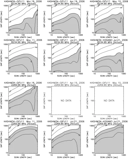
Figure 5 shows contour plots of the standard deviations of φ in a coordinate system where the abscissa repre-sents scan length and ordinate shows gap length the ob-tained from phase structure functions for data of six base-lines from the five sessions. The upper six panels are for 8234.99 MHz and the lower six for 2269.99 MHz. Figure 6 shows the same contour plots as Fig. 5 but for standard de-viations obtained from the actual linear fitting of the phase data. Shaded areas in the figures represent zones where the standard deviation is less than 90◦, which means phases can be connected without ambiguities with a probability of larger than 95%. For example, if we assume 90◦as a limit for connecting phases and we take 100 s for scan length, the gap length can be about 100 s for 8234.99 MHz and about 200 s for 2269.99 MHz for the March 16 data.
We can see that shaded areas in Fig. 5 coincide well with those in Fig. 6. Figure 7 shows their ratio averaged over
gap lengths between 10 to 1000 s as a function of scan length, with the vertical bars indicating the range of ratio. Although ratios are averaged values, a ratio of unity can be interpreted as an indication that they coincide well with each other. Thus, we consider that the simple model used in this study to calculate standard deviations of φ well explains the condition of phase connection over a gap. This means that if a phase structure function is given, we can estimate an available scan-gap length. If we know a phase structure function on longer time periods from a shorter time range observation, we could control scan length and gap length dynamically in order to get the best performance of the D-VLBI observation. Therefore, we investigate here the possibility of estimating a phase structure function in longer time periods from a shorter time range observation. 3.2 Estimation of a structure function at longer time
periods
According to the Kolmogorov turbulence theory (Tatarskii, 1961), variances of phase fluctuations due to the fluctuations of water vapor delay are proportional to
t5/3 at a short time scale and proportional to t2/3 at a
large time scale; these are called 3-D and 2-D turbulences, respectively. Transient time between 3-D and 2-D tur-bulence is given by the thickness of the wet troposphere divided by mean wind velocity. According to Treuhaft and Lanyi (1987), the change from the short period to long period temporal behavior takes place near 125 s, which corresponds to a thickness of 1 km divided by a mean wind velocity of 8 m/s.
We first investigate whether we can see these character-istics in our fringe phase data or not. In order to obtain a phase structure function contributed by atmospheric origin, we calculate a phase structure function defined as
σ2
T. KONDOet al.: PHASE DELAY CONNECTION IN VLBI 365
Fig. 8. Phase-structure-functions after removal of thermal phase noises for 8243.99 MHz (left panel) and 2269.99 MHz (right panel) for all sessions. Dotted lines show model slopes simulating Kolmogorov turbulences (see text for details).
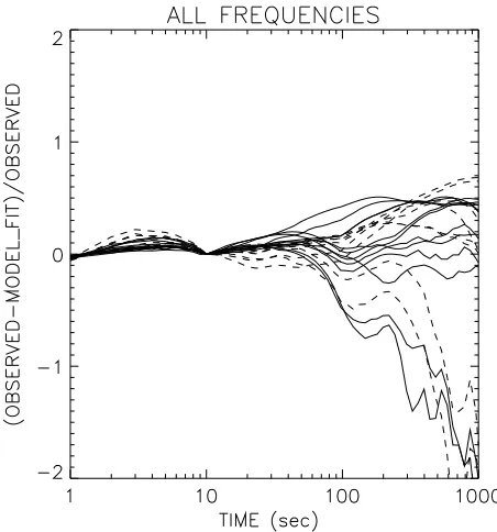
Fig. 9. Relative error of phase-structure-functions estimated from those atτ =10 s for all frequencies and for all sessions. Solid lines are for X-band data and dashed lines for S-band.
whereσ2(0)is the phase variance at the shortest time
inter-val (i.e., 1 s in this study), assuming that this represents a phase noise caused by thermal noise (i.e., related to SNR). Hence,σn2(τ)is thought to be of atmospheric origin,
includ-ing some instrumentation noises as well as a thermal noise. Figure 8 showsσn2(τ) at 8243.99 MHz and 2269.99 MHz
for all sessions. As shown in this figure, σ2
n(τ) seems to
follow the characteristics of Kolmogorov turbulence, i.e., σ2
n(τ)is proportional tot5/3for periods less than 10 s and is
proportional tot2/3for periods longer than 100 s. Although
the absolute value of σ2
n(τ) reflects weather conditions at
every session, the slopes seem to be stable, in particular for periods less than 100 s. Therefore, we modelσn2(τ)using a
piecewise linear function on the log-log plot as follows,
ˆ
σ2
n(τ)=CiτBi (23)
with the following boundary condition,
Cit Bi
i+1=Ci+1t Bi+1
i+1 (24)
where i is an index representing the time range of ti ∼ ti+1 and Ci is a parameter to be fitted for time range ti. Bi is a fixed parameter, i.e., Bi is not estimated, but only Ci is estimated. Therefore, ifσn2(τ) is given at a certain
τ, we can determine all Cis using the relation given by
Eq. (24). This means thatσn2(τ)at a longer time scale can
be inferred from that at a shorter time scale. Thus, if the fringe phase is observed in real-time, we can estimate an available scan-gap limit in real-time, and the most suitable scan length and scan gap for D-VLBI observations, which will depend on weather conditions during the observation, can be determined dynamically. Once a phase structure function contributed by atmosphere is inferred, an overall phase structure function can be given by adding an SNR phase noise as
ˆ
σ2(τ)=2σ2 SNRu+ ˆσ
2
n(τ) (25)
whereσSNRuis a phase error due to a thermal noise of a unit
integration period.
An actual procedure to obtainσˆn2(τ)is as follows. We
use three time ranges, 1–10, 10–100, 100–1000 s, so thatt1,
t2,t3, andt4are 1, 10, 100, and 1000, respectively. Param-eterC2, i.e.,C at the second time range, is first calculated
using realσ2
n(τ)observed forτ =10 s. ParametersC1and C3are then calculated using Eq. (24). For parameterBis for
366 T. KONDOet al.: PHASE DELAY CONNECTION IN VLBI
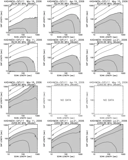
Fig. 10. Same as Fig. 5 but obtained by Kolmogorov model fitting. See text for details.
turbulences. Figure 9 shows relative errors of σˆ2(τ) esti-mated this way for all frequencies and for all sessions. We can then calculate standard deviations ofφusing obtained
ˆ
σ2(τ). Results are shown in Fig. 10.
4.
Results and Discussion
Fringe phase data used in this study are those obtained af-ter the removal of linear and second order trend for a whole observation period of 3600 or 7200 s, in other words, fluctu-ations with a time scale longer than a few thousand seconds are smeared out. However, the time scale concerned in this study is shorter than 1000 s, so that removal of the trend
does not affect the results of this study.
Equation (18) calculates the variance ofφas a function of scan length and gap length from a phase structure func-tion. It is derived from a simple model. Assumptions used in the model are summarized as follows.
A1) Neglecting cross-terms ofak, εk, andεk+1 to derive
Eq. (8) from Eq. (7);
A2) Use of a theoretical fitting error based on a normal dis-tribution variable in Eq. (11) to simplify the problem; A3) Use of phases only att=tkandtk+tsto deriveσa2in
T. KONDOet al.: PHASE DELAY CONNECTION IN VLBI 367
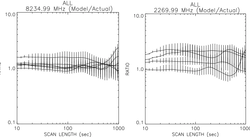
Fig. 11. Same as Fig. 7 but for ratios of standard deviation of phase errors obtained from phase structure functions obtained by the Kolmogorov model fitting and those obtained from actual linear fitting for 8234.99 MHz (left panel) and for 2269.99 MHz (right panel).
Fig. 12. Same as Fig. 7 but for ratios of standard deviation of phase errors obtained from actual phase structure functions and those obtained by Kolmogorov model fitting for 8234.99 MHz (left panel) and for 2269.99 MHz (right panel).
A4) Assuming a normal distribution variable (thermal noise) only to express an SNR integrated over the whole scan length in Eq. (15);
A5) Obtaining σφ from a phase structure function at the shortest time scale in Eq. (17).
Regarding A1, we have computed the magnitude of cross-terms and the ratio to the total term to check the valid-ity of this assumption. The last term of the right hand side of Eq. (7) sometimes shows a ratio exceeding 0.5; however, the root of absolute value is less than 30◦ for most of the combinations of scan and gap lengths. Therefore, this
as-sumption can affect the results by about a few tens of de-grees. A2 usually underestimates a fitting error at the end of the scan period for actual phase fluctuations at the time scale concerned in this study.
A3 gives the overestimation in the case of a normal distri-bution variable. A4 overestimates an SNR for actual phase fluctuations. A5 overestimatesσφbecause a phase structure function at the shortest time scale (now it is 1 s) may include the fluctuations due to the propagation media even though it is thought to be small enough.
fit-368 T. KONDOet al.: PHASE DELAY CONNECTION IN VLBI
Fig. 13. Scatter plots of gap limits obtained from Kolmogorov model and actual linear fitting for all sessions. Top and middle panels are for 8234.99 MHz and bottom for 2269.99 MHz. Standard deviations of 90◦(top panel) and 60◦(middle and bottom panels) are adopted as thresholds to calculate a gap limit under the condition of gap length (tg)=scan length (ts). Plots of the case of standard deviations of 90◦ for 2269.99 MHz are omitted because all available gap lengths exceed 1000 s.
ting results, as shown in Figs. 5 and 6. Their coincidence is demonstrated in Fig. 7, which plots their ratio averaged over gap lengths of between 10 to 1000 s as a function of scan length, with vertical bars indicating the range of the ratio. We can see a good correspondence, particularly for X-band (8234.99 MHz) at periods shorter than 600 s. However, for most cases, the ratio is larger than 1.0 and sometimes ex-ceeds 2.0 for the S-band (2269.99 MHz), i.e., the standard deviation of phase error estimated from the simple model is larger than that obtained from the actual linear fitting. Therefore, the available scan gap is estimated to be shorter than the actual one. In other words, the available gap length is underestimated in comparison with the real one, so that it will ensure the correct connection of phase delay.
Although the model has some defects, it is concluded that we can use Eq. (18) for evaluating the relation between scan length and available gap length from a phase structure function.
The next issue to discuss is how accurately we can esti-mate phase structure functions at longer time periods from those at a shorter time. As shown in Fig. 8, actual phase structure functions at a time period of less than 100 s, espe-cially 10–100 s, are well-characterized by a fixed slope of about 1.0 on the log-log plot. The same quantitative char-acteristics can be seen in Fig. 8 of Liuet al.(2005). Thus, it is expected that the estimation of a whole structure function from that at 10 s will give a reasonable phase structure tion. Actually, as shown in Fig. 9, the whole structure func-tion shows a good correspondence with an observed one. Relative errors are within±0.5 at 10–1000 s except for four lines which correspond to two S-band and two X-band data observed on March 16, 2006 under rain conditions at both stations. Structure functions observed on March 16 show slightly different features than the others, i.e., the slope on the log-log plot at a large time scale is more moderate than the others, and transition to this moderate slope occurs at a time scale shorter than that of the others. This results in the large discrepancy at the large time scale. The results of standard deviations ofφcalculated by an estimated phase structure function is shown in Fig. 10. They coincide well with those obtained by actual linear fittings (Fig. 6). Their ratio is plotted in Fig. 11 with the same format as Fig. 7.
We can see similar characteristics with Fig. 7. From this result, it can be expected that the standard deviations calculated from an actual phase structure function and those based on Kolmogorov model fitting at a short time period coincide well with each other. Actually, their difference is less than a factor of 2 at time periods 10–1000 s, as shown in Fig. 12. We therefore conclude that we can infer a fairly accurate phase structure function at longer time periods by using σ2(τ) at τ = 10 s and we can use it to estimate
standard deviations ofφ.
T. KONDOet al.: PHASE DELAY CONNECTION IN VLBI 369
Fig. 14. Scatter plots of fringe phases of 8234.99 MHz and 2269.99 MHz observed on March 16 (left panel) and on May 11 (right panel), 2006.
90◦for 2269.99 MHz are omitted because all available gap lengths exceed 1000 s. As shown in this figure, both lim-its coincide fairly well with each other. Actual gap limlim-its vary significantly session by session from about 50–230 s for a standard deviation of 90◦ and 20–110 s for 60◦ at 8234.99 MHz. As for 2269.99 MHz, they exceed 1000 s for 90◦ and 250–700 s for 60◦. The range of gap limits in the case of a standard deviation of 90◦ is consistent with Beasley and Conway’s (1995) prediction of 160–440 s for switching time (that is about double the gap length) at a fre-quency of 8.4 GHz, which is based on the 90◦ criterion. They are also consistent with the VLBA’s recommenda-tion on a phase referencing observarecommenda-tion at frequencies 1.4– 8.4 GHz, which is a switching time of 300 s (180 s on a target and 120 s on a calibrator).
As shown in Fig. 13, available gap lengths for the S-band are usually longer than those for the X-band. The delay fluctuations caused by the troposphere are independent of frequency, while those caused by the ionosphere are written inversely as the square of the frequencies. We usually see a good positive correlation between S-band phase fluctua-tions and X-band ones, as shown in the left panel of Fig. 14. The magnitude of the fluctuations of the S-band is about one-fourth of that of the X-band, so that it can be concluded that such fluctuations are caused by the non-dispersive de-lay change due to the troposphere. We therefore consider that the idea of connecting X-band data using phase delay data observed for S-band will work well for this case. How-ever, there is a case which indicates hysteresis-like fluctu-ations and suggests the existence of uncorrelated compo-nents, as shown in the right panel of Fig. 14. Instrumenta-tion, ionosphere, and solar wind plasma can cause such un-correlated components. In particular, scintillations caused by the solar wind affects phase fluctuations at an S-band larger than those at the X-band. An area affected by large scintillations (scintillation index> 0.1) at the S-band ex-ceeds an angle distance of 10◦from the sun at solar maxi-mum (Tokumaruet al., 1995). Therefore, the connection of fringe phases at the X-band using S-band fringe phase data
is thought not to work adequately in some cases, such as in the case of solar maximum at an area close to the sun. This issue, although very interesting, is far beyond the scope of this paper and will not be discussed here.
In the case of D-VLBI, which observes two celestial ra-dio sources alternately, a scan period for a source corre-sponds to a gap period for the other source. In practice, the time of antenna motion necessary for source change should be considered as a part of the gap period. Lettcbe a time required to change the source, a necessary condition to be satisfied by a gap lengthtgis given by
tg≥ts+2tc. (26)
A solution can be obtained, for example, graphically by plotting Eq. (26) on Fig. 10. However, we will not discuss these results here because the purpose of this study is to evaluate the possibility of scan-gap limit from a structure function obtained at a short time period.
370 T. KONDOet al.: PHASE DELAY CONNECTION IN VLBI
Lastly, we discuss about an accuracy requirement. According to Thornton and Border (2003), a require-ment for the angular position measurerequire-ment of a spacecraft is 50 nrad during interplanetary cruise phases and 5–10 nrad to deliver landers on the surface of Mars. For example, 5 nrad as a requirement for the measurement accuracy cor-responds to a one-sigma delay error of 5 ps for a projected baseline length of 300 km (close to Kashima-Gifu baseline length). This is not a difficult requirement even for narrow bandwidth signals from a spacecraft if we can measure a phase delay without ambiguities, because 5 ps corresponds to 14.4◦at 8 GHz and it is easily achieved by observations ofSNR>4 (see Eq. (14)). However, this is for an ideal case in which common error sources, such as those introduced by receiving systems, clocks, propagating media, and sta-tion locasta-tions, can be completely cancelled by D-VLBI, and phase delays can be connected without ambiguities among consecutive scans over a gap.
In other words, we suggest that it is possible to measure an angular position of spacecraft by D-VLBI on a short baseline, such as 300 km, with an accuracy meeting with a requirement for a Mars lander if the use of phase delay is realized through the phase delay connection among consec-utive scans.
Discussions on the accuracy requirement described above are for the case that the phase-delay connection is achieved perfectly without any ambiguities. Failure in the phase-delay connection between consecutive scans intro-duces a bias error equal to an ambiguity in observed delay (we suppose minimum ambiguity here for simplicity). An effective bias error will be given by a simple weighted mean regarding the number of scans accompanied by an ambigu-ity. However, we do not know where the phase-delay con-nection fails in the case of (i.e., one-baseline) observations made at two stations (a failure in phase-delay connection may be found through the “closure phase” method in the case observations made at three or more stations). If the phase-delay connection fails at the last scan, an effective bias error will be small. If it fails at the second scan, an ef-fective bias error keeps a large value close to an ambiguity. Although an effective bias varies in this way, we can con-sider the half of ambiguity as an effective bias error when the phase-delay connection fails only once in a series of scans. An ambiguity is 125 ps at 8 GHz, so that an effective bias can be considered as 62.5 ps, and it is larger than the re-quired accuracy on the short baseline described above. Let the probability of failure in the phase-delay connection be P, and the number of scans where phase-delay connection fails is thought to be given by PN where N is the total num-ber of scans. P is 5% for the 90◦criterion and 0.3% for the 60◦criterion. Therefore, 20 scans include at least one scan where the phase-delay connection fails in the case of the 90◦ criterion and 333 scans for the 60◦criterion. Based on ac-tual available gap limits (50–230 s for the 90◦criterion and 20–110 s for the 60◦ criterion at 8234.99 MHz), the total scan number can exceed 20 in the case of the 90◦criterion. Thus, the 60◦criterion is thought to be more preferable for an actual application.
5.
Conclusions
We have carried out a series of VLBI experiments in 2006 using three stations, Kashima, Gifu, and Koganei to investigate the relation between scan length and scan gap limit.
Our first step has been to develop a simple method to evaluate a scan gap limit based on the error analysis of lin-ear fitted data using a phase structure function. This has been derived from a simple assumption regarding the error of phase changing rate, i.e., the error is described only by the phase difference at the both ends of scan period. Stan-dard deviations of phase errors over a gap estimated by this method have been compared with those estimated from an actual linear fitting of fringe phases, and the validity of the simple method developed in this study has been confirmed. However, in most cases, the available scan gap estimated from the simple model is a bit shorter than the actual one. This means that the improvement of the model will give a more correct scan-gap length, but we leave this for a future study.
As for the possibility of the estimation of a whole struc-ture function from that at a short time period, which is nec-essary for dynamic scheduling at D-VLBI, a model based on the Kolmogorov turbulence theory has been proposed. We model a phase structure function depending on the wet atmosphere by using a piecewise linear function on the log-log plot; a phase structure function follows a power law having three different slopes 1.67 (= 5/3), 1.00, and 0.67 (= 2/3) for three time ranges, 1–10, 10–100, and 100– 1000 s, respectively. Since the function is continuous at boundaries, the model can estimate a structure function at τ >100 s from that atτ =10 s. The validity of the model has been confirmed by a comparison of standard deviations of phase errors over a gap estimated from a structure func-tion obtained by this model and those estimated from an actual linear fitting of fringe phases. Hence, it can be con-cluded that we can estimate a fairly accurate phase structure function at longer time periods by using that atτ = 10 s, and we can use it to estimate standard deviations of phase error over a scan gap. This suggests that it is possible to control scan length and gap length dynamically in order to achieve the best performance for D-VLBI observations.
Acknowledgments. A part of this work was carried out during a temporary stay by one of authors (TK) at the Vienna University of Technology (TU). He thanks Harald Schuh, head of the Institute of Geodesy and Geophysics, TU, for supporting his stay. This research was supported in part by the research project P16136-N06 “Investigation of the ionosphere by geodetic VLBI” founded by the Austrian Science Fund (FWF).
References
Beasley, A. J. and J. E. Conway, VLBI phase-referencing, inVery Long Baseline Interferometry and the VLBA, ASP Conf. Ser.82, edited by J. A. Zensus, P. J. Diamond, and P. J. Napier, 327–343, 1995.
Border, J. S. and J. A. Koukos, Technical characteristics and accuracy ca-pabilities of delta differential one-way ranging (DOR) as a spacecraft navigation tool, CCSDS B20.0-Y-1,Report of the Proceedings of the RF and Modulation Subpanel 1E Meeting at the German Space Opera-tions Centre: September 20–24, 1993, edited by T. M. Nguyen, Yellow Book, Oberpfaffenhofen, Germany: Consultative Committee for Space Data Systems, February, 1994.
T. KONDOet al.: PHASE DELAY CONNECTION IN VLBI 371 S. Christensen, and D. E. Hilt, Delta VLBI spacecraft tracking system
demonstration: Part I. design and planning,DSN Progress Report 42-45, 111–132, 1978.
Christensen, C. S., B. Moultrie, P. S. Callahan, F. F. Donivan, and S. C. Wu, Delta VLBI spacecraft tracking system demonstration: Part II: data acquisition and processing,TDA Progress Report 42-60, 60–67, 1980. Fujiwara, A., T. Mukai, J. Kawaguchi, and K. T. Uesugi, Sample return
mission to NEA: MUSES-C,Advances in Space Research,25, 231–238, 1999.
Ichikawa, R., M. Sekido, H. Osaki, Y. Koyama, T. Kondo, T. Ohnishi, M. Yoshikawa, W. Cannon, A. Novikov, M. Berube, and NOZOMI DVLBI GROUP, An evaluation of VLBI observations for the deep space tracking on the interplanetary spacecrafts, inInternational VLBI Service for Geodesy and Astrometry 2004 General Meeting Proceedings, edited by Nancy R. Vandenberg and Karen D. Baver, NASA/CP-2004-212255, 253–257, 2004.
Ichikawa, R., M. Sekido, Y. Koyama, and T. Kondo, An evaluation of at-mospheric path delay correction in differential VLBI experiments for spacecraft tracking, inInternational VLBI Service for Geodesy and As-trometry 2006 General Meeting Proceedings, edited by D. Behrend and K. D. Baver, NASA/CP-2006-214140, 226–230, 2006.
Kasuga, T., M. Ishiguro, and R. Kawabe, Interferometric measurement of tropospheric phase fluctuations at 22 GHz on antenna spacings of 27 to 540 m,IEEE Trans. Antennas Propag.,AP-34, 797–803, 1986. Kikuchi, F., Y. Kono, M. Yoshikawa, M. Sekido, M. Ohnishi, Y. Murata,
J. Ping, Q. Liu, K. Matsumoto, K. Asari, S. Tsuruta, H. Hanada, and N. Kawano, VLBI observation of narrow bandwidth signals from the spacecraft,Earth Planets Space,56, 1041–1047, 2004.
Kondo, T., Y. Koyama, J. Nakajima, M. Sekido, and H. Osaki, Internet VLBI system based on the PC-VSSP (IP-VLBI) board, inNew Tech-nologies in VLBI, ASP Conf. Ser.306, edited by Minh, Y. C., 205–216, 2003.
Kondo, T., M. Kimura, Y. Koyama, and H. Osaki, Current status of soft-ware correlators developed at Kashima Space Research Center, in Inter-national VLBI Service for Geodesy and Astrometry 2004 General Meet-ing ProceedMeet-ings, edited by Nancy R. Vandenberg and Karen D. Baver, NASA/CP-2004-212255, 186–190, 2004.
Kono, Y., H. Hanada, J. Ping, Y. Koyama, Y. Fukuzaki, and N. Kawano, Precise positioning of spacecrafts by multi-frequency VLBI, Earth Planets Space,55, 581–589, 2003.
Koyama, Y., T. Kondo, M. Kimura, H. Takeuchi, and M. Hirabaru, e-VLBI developments with the K-5 system, inInternational VLBI Service for Geodesy and Astrometry 2006 General Meeting Proceedings, edited by D. Behrend and K. D. Baver, NASA/CP-2006-214140, 216–220, 2006. Liu, Q., M. Nishio, K. Yamamura, T. Miyazaki, M. Hirata, T. Suzuyama, S. Kuji, K. Iwadate, O. Kameya, and N. Kawano, Statistical characteristics
of atmospheric phase fluctuations observed by a VLBI system using a beacon wave from a geostationary satellite,IEEE Trans. Antennas Propag.,AP-53, 1519–1527, 2005.
Rogers, A. E. E., Very-long-baseline interferometry with large effective bandwidth for phase-delay measurements,Radio Sci.,5, 1239–1247, 1970.
Rogers, A. E. E. and J. M. Moran, Coherence limit for very long baseline interferometry,IEEE Trans. Instrum. Meas.,IM-30, 283–286, 1981. Rogers, A. E. E., A. T. Moffet, D. C. Backer, and J. M. Moran, Coherence
limits in VLBI observation at 3-millimeter wave length,Radio Sci., 19, 1552–1560, 1984.
Sekido, M., R. Ichikawa, H. Osaki, T. Kondo, Y. Koyama, M. Yoshikawa, T. Ohnishi, W. Cannon, A. Novikov, M. Berube, and NOZOMI DVLBI GROUP, VLBI observation spacecraft navigation (NOZOMI)—data processing and analysis status report, inInternational VLBI Service for Geodesy and Astrometry 2004 General Meeting Proceedings, edited by Nancy R. Vandenberg and Karen D. Baver, NASA/CP-2004-212255, 258–262, 2004.
Takahashi, F., T. Kondo, Y. Takahashi, and Y. Koyama,Very long baseline interferometer, Ohmsha, Tokyo, 2000.
Tatarskii, V. I.,Wave Propagation in a Turbulent Medium, Dover, New York, 1961.
Thornton, C. L. and J. S. Border,Radiometric tracking techniques for deep-space navigation, John Wiley & Sons. Inc., Hoboken, New Jersey, 2003.
Tokumaru, M., H. Mori, T. Tanaka, and T. Kondo, Evolution of the So-lar Wind Structure in the Acceleration Region during (STEP Interval) 1990–1993,J. Geomag. Geoelectr.,47, 1113–1120, 1995.
Treuhaft, R. N. and G. E. Lanyi, The effect of the dynamic wet troposphere on radio interferometric measurements,Radio Sci.,22, 251–265, 1987. Whitney, A. R. and C. A. Ruszczyk, e-VLBI development at Haystack Observatory, inInternational VLBI Service for Geodesy and Astrometry 2006 General Meeting Proceedings, edited by D. Behrend and K. D. Baver, NASA/CP-2006-214140, 211–215, 2006.
Wrobel, J. M., R. C. Walker, J. M. Benson, and A. J. Beasley, VLBA scientific memorandum 24: Strategies for phase referencing with the VLBA, http://www.vlba.nrao.edu/memos/sci/sci24memo.ps, 2000. Wu, S. C., Connection and validation of narrow-band delta VLBI phase
observations,DSN Progress report 42-52, 13–20, 1979.
Yamamoto, T. and K. Tsuruda, The PLANET-B mission,Earth Planets Space,50, 175–181, 1998.