A SURVEY ON THE CURES FOR THE CURSE OF DIMENSIONALITY IN BIG DATA
RESHMA REMESH
1*, PATTABIRAMAN V
2*
1Department of Computer Science & Engineering Specialization in Big Data Analytics, VIT University, Chennai, Tamil Nadu, India. 2Department of Computer Science & Engineering, VIT University, Chennai, Tamil Nadu, India.
Email: [email protected]/[email protected]
Dimensionality reduction techniques are used to reduce the complexity for analysis of high-dimensional data sets. The raw input data set may have large dimensions, and it might consume time and lead to wrong predictions if unnecessary data attributes are been considered for analysis. Hence, using dimensionality reduction techniques, one can reduce the dimensions of input data toward accurate prediction with less cost. In this paper, the different machine learning approaches used for dimensionality reductions such as principal component analysis (PCA), singular value decomposition, linear discriminant analysis, Kernel PCA, and artificial neural networkhave been studied.
Keywords: Dimensionality reduction, Principal component analysis, Singular value decomposition, Linear discriminant analysis, Kernel principal component analysis, Artificial neural network.
INTRODUCTION
Analyzing and processing of high-dimensional data are a tedious task and consumes large amount of time; these are among the major challenges in big data [1]. The higher dimensionality of the data might have a negative impact while applying for many of the clustering algorithms. Hence to address the curse of dimensionality of the data, we introduce dimensionality reduction techniques. Thus, dimensionality reduction techniques is been done as a data pre-processing step before applying any of these algorithms in such a way that it will not compromise the accuracy of the results. Feature extraction and feature selection are two types of dimensionality reduction methods. Essential features are extracted from the original input dataset in case of feature extraction method. The feature extraction method reduces the dimensionality by transforming the original dataset features into a new reduced set of features. While in feature selection method a subset of the already existing features are been selected [2]. Supervised approach and unsupervised approach are the two approaches available for dimensionality reduction.
Dimensionality reduction is the process by which we can convert large dimensional dataset into data with lesser dimensions, but it makes sure that it conveys the same information concisely. It can be used for data compression, reduce storage space, reduce the time required for analyzing and performing computations and helps in better visualization of the data. We can use either supervised approaches or unsupervised approaches for dimensionality reduction techniques. Linear discriminant analysis (LDA), neural network is some of the supervised dimensionality reduction techniques. Principal component analysis (PCA), singular value decomposition (SVD), and kernel PCA (KPCA) are few of the unsupervised approaches of dimensionality reduction.
Microarray data analysis, face recognition, protein classification, text mining, image retrieval are some of the real-time applications of dimensionality reduction techniques.
LITERATURE SURVEY
Bae et al. [3] in their paper used the PCA method to analyze the age-related factors of wrist pulse from various analysis parameters. The wrist pulse signals and respiratory signals from 40 people, 20 each in the age group of 20s and 40s who do not have any cardiovascular
disorders were included for their study. The PCA was performed on twenty different analysis parameters that can reflect pulse characteristics. From among these parameters, the parameters which were expected to contain information regarding the age-related factors have to be examined. After performing PCA, the newly transformed analysis parameters with lower dimensions were used to obtain the differences in the age group of these people by evaluating the score of the principal components (PCs). The MATLAB R2015b software was made use of to do the same. The experiment showed that there was different dispersion among the two age groups which means that there exist age-related parameters in wrist pulse signals. Once the statistical difference between these two age groups were been analyzed the score of first PC of age group 20 were much lower than that of age group 40. However, the other higher PCs did not show much statistical difference between the two age groups once when they were tested. Hence, they came to the conclusion that the first PC could be considered as an age-related factor of the wrist pulse and it can be used to classify the typical pulse with age.
Seng et al. [4] proposed a paper in which the rule-based and machine learning strategies are been used together to solve the problem of audio-visual emotion recognition. The emotions of people are been recognized by giving their audio and visual data as the input. ORL, YALE (standard face recognition databases), Cohn-Kanade dataset (visual emotion recognition dataset), eNTERFACE’05, RML (audio-visual emotion database) are the different databases that has been used for the experiments in this paper. The high dimensional data are been transformed to low-dimensional data, and the classes are been separated with bidirectional principle component analysis and least square LDA for the design of the visual path and the transformed features are then passed through an optimized kernel laplacian radial basis function neural classifier. Moreover, for the design of audio path the rhythmic and spectral features are combined, and these transformed audio features are then channeled through an audio feature level fusion module. The outputs from both the audio and visual path are been combined using the score-level fusion method in the audio-visual fusion module. As a final step the emotions recognized from above audio path, visual path steps are been analyzed along with the one obtained after the fusion of those outputs and the score is been analyzed, and the emotion that has the maximum score will be considered as the final output.
© 2017 The Authors. Published by Innovare Academic Sciences Pvt Ltd. This is an open access article under the CC BY license (http://creativecommons. org/licenses/by/4. 0/) DOI: http://dx.doi.org/10.22159/ajpcr.2017.v10s1.19755
Received: 19 January 2017, Revised and Accepted: 20 February 2017
Fuadi et al. [5] the objective of this paper is to analyze the document clustering quality when SVD technique is used for the dimensionality reduction. Here to reduce the dimension of the document, the SVD method is applied to the term-document matrix and thus the matrix is factorized into three matrices and from these matrices the least singular values are set to zero and thus the rows formed from these singular values can be eliminated and thus the dimensionality of the matrices can be reduced and in such a way only the most relevant values are been selected and the other terms are neglected. Then using the k-means algorithm clusters are been formed out of the data, and then the quality of these data clusters are been checked to check whether there is drastic change in the quality when the dimensionality is been reduced. The quality check shows that there is not much change in the quality of data clusters after dimensionality reduction when compared to the clusters when all the dimensions are been considered.
Ibrahim et al. [6] in their paper used an intelligent multi-objective classifier and tried to classify and diagnose breast cancer disease using multilayer perceptron NN with differential evolution technique. In multilayer perceptron, a set of inputs gets mapped to a set of output. It is an artificial feedforward NN. Here the real DE algorithm is changed in such a way that it can be applied for multi-objective optimization problem. Multi-objective optimization algorithm is used to optimize the conflicting objectives simultaneously based on some constraints. In this study, breast cancer, dataset was used and they tried to classify the data or the tumor as belonging to malignant or benign. There were nine attributes for the dataset and benign and malignant was the two output classes. The intelligent multi-objective classifier used the objective evolutionary algorithm, and it was based on the multi-objective differential evolution algorithm and the artificial NN (ANN) on the multilayer perceptron NN. The NNs hidden nodes in hidden layers were been optimized here using multi-objective differential evolution algorithm. Here, the method depends on two objective functions, and the goal was to minimize these functions. One function was to improve accuracy or the performance by reducing the error rate in the network for the training data, and the other was to reduce the number of hidden nodes in the network and thus reduce its complexity. From the experiment, a good classification for the training and testing dataset for the diagnosis of breast cancer was obtained, the classifier was able to classify the benign and malignant tumors of breast cancer well, and it also produced a simple network structure with the lowest complexity. EXISTING TECHNIQUES
In dimensionality reduction techniques, there are supervised and unsupervised algorithms. In supervised method, the class labels are retained. The class to which each attribute belongs are all retained in the training dataset and based on the training dataset the new data are classified. In unsupervised method the class labels are unknown. It tries to find a the structure that can explain the original data [7].
PCA
PCA is one of the prominent strategies among unsupervised feature extraction technique. It is a statistical procedure. The variables in the data go through orthogonal transformation and are transformed into a set of uncorrelated variables that captures most of the variance in the data and are called as PCs [8]. The PCs may be equal or less in number to the original set of attributes. Few orthogonal linear combinations of the existing attribute having the largest variance are been found out and using it the number of attributes of the data are reduced. These orthogonal linear combinations are called as the PCs. Most of the variance will be explained by first PCs [9] hence even though we remove the rest of the PCs there will not be much reduction in information in most of the datasets [10] thus dimensionality reduction of the attributes becomes easy.
SVD
SVD is a matrix factorization method for low-rank approximation [5]. A matrix of rank R is reduced to a matrix of rank K. The R matrix considered as a list of R unique vectors, and it can be approximated as a linear combination of K unique vectors. Each row can be written as sum of
vectors like,
Ri=ciSV1+biSV2 +…. (1)
Where, ci is scale factor and SV1, SV2 are singular vectors with highest
and second highest singular values. Here, a matrix M is been factorized into three matrices M=UDVT here the columns of matrices U and V are
orthonormal, and matrix D is diagonal. If the matrix to be factorized is too large and also the matrices U, D, and V formed are also large such that it is not convenient to store them, then the dimensionality of these three matrices can be reduced by setting the least singular values to zero [11]. The rows that are formed from these singular values can be eliminated from U and V once these least singular values are set to zero. Thus, SVD is used for elimination of less important features and by that way to get the desired number of dimensions.
Steps to perform SVD:
Find the transpose of a matrix say, A
Calculate X= ATA
Find Eigenvalues for the above matrix, i.e., evaluate ATA-λI
Calculate singular values s1, s2 etc. s=√λ
Arrange the singular values in increasing order.
The singular values are placed in descending order, and a diagonal matrix S is constructed. S−1 is constructed by computing the inverse of
this diagonal matrix S.
Substitute value of Eigenvalues in the equation,
(ATA−λI)X
1=0 (2)
And compute the values of Eigenvectors, Substitute the Eigenvectors for V,
V=[x1 x2]
Find transpose of V to form VT
Calculate U, U=AVS−1
KPCA
KPCA uses the kernel method strategies [2,12]. With a nonlinear transform x→Φ(x) the input data x is changed from its original input space to a higher dimensional feature space. Here Φ is a nonlinear function, and this is to make the nonlinear data become linearly separable. Then a kernel matrix K is formed using the inner products of features of the newly formed transformed data. Then PCA is performed
on the centralized K, i.e.,
K covariance matrix of new feature vectors in the new higher dimensional feature space. PCA does not efficiently represent larger and nonlinear representation of input data. With KPCA method the representation of such kind of input data becomes possible.
LDA
It computes the within-class scatter matrix and between-class scatter matrix for all class samples.
1. Within class scatter matrix,
2. Between class scatter matrix,
= discriminant principle that is to maximize the ratio: (det|Sb|)/(det|Sw|).
To maximize this ratio the value of between class scatter matrixes of projected samples must be maximized and within class scatter matrix must be minimized.
ANN
ANN, here essential features of information processing capabilities of our nervous system is been analyzed, and accordingly, ANN tries to design models for processing the information. In our biological nervous system, the different signals from the body are coded and processed, and proper response is evoked instantly. So likewise in ANN, it tries to imbibe the properties of the nervous system to be able to produce proper responses to the signals that it receives. In ANN each unit can be connected to any other unit similar to the neurons being interconnected in biological networks. The neurons get several input and it performs computation depending on the primitive function mentioned on the body of the neurons and depending on the threshold value mentioned the network decides whether to signal an output or not. Each of the input channels will have a weight associated with it, and at the neuron all the information that are been passed are integrated, and the primitive function f, defined is evaluated. The ANN is thus a collection of such networks of primitive function each of which produces an output which may be transferred to the next level. The ANN learns by example. The network consists of three layers an input layer, hidden layer, and output layer [11]. The input layer consists of the raw information that is passed on to the network, and this input layer is connected to the hidden layer. The activities that are in the hidden layer depend on the input units and the weight that is associated with the connection between each of input unit and hidden unit. The hidden units are in turn connected to the output unit, and its response depends on the activity that is mentioned in the hidden unit and the weight defined in the connection between input and hidden unit. The weight defined in between the connection of input unit and hidden unit can determine when each of the hidden unit is to be active, thus by changing that weight, what each of the hidden unit has to represent can be determined. With time the ANN train itself and thus from the pattern of the input given to train it, the associated output can be taken from the memory and given as output and even the ANN train itself to give output to inputs that have patterns which are not same but similar to the one it is trained for.
EXPERIMENTS AND RESULTS
The PCA method has been studied and implemented. By this method, the most significant variables are found from the large set of variables in the original dataset. From the higher dimensional dataset, the low-dimensional set of variables is pulled out in such a way that these variables can get as much information as possible. The analysis, processing and visualization of data also become easy once the dimensionality has been reduced. The original data are been transformed to a new set. We find the PCs which is a linear combination of the features of the dataset. The first
PC gets the maximum variance from among the original dataset [3,11]. The second PC is also a linear combination of the attributes of data as the first PC, and it gets the remaining variance from the data that has not been captured by the first PC. In such a manner the PCs are found out, and the components with largest values are been selected since larger the value of PC larger the variance in the data that it covers [14]. The remaining lower valued components are neglected since they do not contribute much to the variance in the original dataset. These selected components are then used to compute the new transformed dataset with reduced dimensionality.
Performing PCA in R on iris dataset:
This iris dataset contains 150 instances, 50 each of three classes of an iris plant. It has five attributes, namely, Sepal.Length, Sepal.Width, Petal.Length, Petal.Width, Class/Species. Class/species is a categorical attribute has three categories Iris setosa, Iris virginica, Iris versicolour. Here, we try to find which all attributes are required to predict the class/species of the iris plant and can be used to capture most of the information from the original dataset.
Pseudo code of PCA using R:
Step 1:
Calculating mean for all the numerical attributes
mean_var=mean(variable) Step 2:
Normalize the data
Norm_var=orginal_variable–mean_variable (5)
Step 3:
Create a data frame, the adjusted or normalized dataset
new_variable=data.frame(variable1,variable2,…) Step 4:
Find transpose of the adjusted data
tran_new=t(new_variable) Step 5:
Find covariance matrix of this adjusted data cov_new=cov(new_variable)
Step 6:
Find Eigenvalues from this covariance matrix
eigen_var=eigen(cov_new) Step 7:
From the above result, its evident that the Sepal.Length and Sepal. Width has highest eigenvalues hence their corresponding Eigenvectors can be considered. These would capture the maximum variance from the whole data set.
Find the feature vector, i.e., the Eigenvectors corresponding to first two Eigenvalues is been considered as a separate data frame.
Step 8:
Find the transpose of the feature vector trans_fvector=t(feature_vector)
Step 9:
Find the final dataset
finalset=transp_fvector*trans_new Step 10:
Find the transpose of final dataset to view the dimension reduced transformed data
trans_final=t(final set)
Here in the transformed data, the number of attributes has been meanSeL=mean (iris1$Sepal.Length)
//To find the mean of all attributes meanSeW=mean (iris1$Sepal.Width) meanPeL=mean (iris1$Petal.Length) meanPeW=mean (iris1$Petal.Width) meanSeL
//the mean value of Sepal.Length [1] 5.843333
meanSeW
//the mean value of Sepal.Width [1] 3.057333
meanPeL
//the mean value of Petal.Length [1] 3.758
meanPeW
//the mean value of Petal.Width [1] 1.199333
//normalize the value of each attribute normSeL=iris1$Sepal.Length-meanSeL //normalize the value of Sepal.Length
Table 1: Sample of iris dataset
SL SW PL PW Species
5.1 3.5 1.4 0.2 Setosa
4.9 3 1.4 0.2 Setosa
4.7 3.2 1.3 0.2 Setosa
4.6 3.1 1.5 0.2 Setosa
5 3.6 1.4 0.2 Setosa
SL: Sepal.Length, SW: Sepal.Width, PL: Petal.Length, PW: Petal.Width
normSeW=iris1$Sepal.Width-meanSeW normPeL=iris1$Petal.Length-meanPeL normPeW=iris1$Petal.Width-meanPeW
//Refer Table 2 for sample output of normalized values adj=data.frame (normSeL, normSeW, normPeL, normPeW) //Creating a dataframe with the
normalised values trans_adj=t (adj)
//To find the transpose of the dataframe created
cov_adj=cov (adj)
//To find the covariance value of the adjusted dataframe cov_adj
//Refer Table 3 to view the output eigen_adj=eigen (cov_adj)
//To find the eigen value and vector eigen_adj$values
//The first row gives the eigenvalues and the rows below display the feature vector
4.22824171 0.24267075 0.07820950 0.02383509 //Eigen values
feature_vec=data.frame (eigen_adj$vectors [,1:2])
//Taking the first two vectors formed from the first two eigen values and creating a dataframe
feature_vec
//Refer Table 4 to view the feature vector transp_feature=t (feature_vec)
//To find the transpose of the feature-vector transp_feature
//Refer Table 5 for output
finaldata=transp_feature%*%trans_adj
//Multiply the transpose of feature vector with the transpose of adjusted data frame to get final data
final=t (finaldata)
//To find transpose of the finaldata > head (final)
//Refer Table 6 to view output
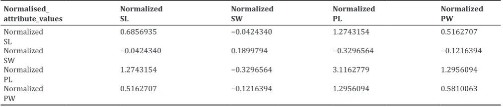
Table 3: Covariance values of the data adjusted data frame Normalised_
attribute_values NormalizedSL NormalizedSW NormalizedPL NormalizedPW
Normalized
SL 0.6856935 −0.0424340 1.2743154 0.5162707
Normalized
SW −0.0424340 0.1899794 −0.3296564 −0.1216394
Normalized
PL 1.2743154 −0.3296564 3.1162779 1.2956094
Normalized
PW 0.5162707 −0.1216394 1.2956094 0.5810063
SL: Sepal.Length, SW: Sepal.Width, PL: Petal.Length, PW: Petal.Width
Table 2: Sample of normalized values of attributes in iris dataset
Attribute_names 1 2 3 4 5 6
SL −0.7433333 −0.9433333 −1.1433333 1.2433333 −0.8433333 −0.4433333
SW 0.44266667 −0.05733333 0.14266667 0.04266667 0.54266667 0.84266667
PL −2.358 −2.358 −2.458 −2.258 −2.358 −2.058
PW −0.9993333 −0.9993333 −0.9993333 0.9993333 −0.9993333 −0.7993333
reduced to two. Hence, using these two attribute values itself major
information of the original dataset can be captured and can be used to predict the class of iris if required.
RESULTS
In this Table 1, it provides a sample of the data after the values are normalized. After normalization, the mean of the attribute becomes equal to zero.
Table 3 gives the covariance values of attributes to each other from the normalized dataset.
Eigenvector formed from the PCs is been treated as a new feature vector. X1, X2 gives the Eigenvector values (Tables 4 and 5).
The final data are the product of the transpose of newly formed feature vector and the transpose of the row adjusted data (normalized dataset) (Table 6).
PCA on arrhythmia dataset
Arrhythmia dataset contains information about cardiac arrhythmia disease. There are 452 instances and 279 attributes in this dataset, the last column is the class variable. This data can be classified into one of the 16 groups. Class 1 refers to normal ECG, Class 2-15 refers to different classes of arrhythmia and Class 16 refers to the rest of unclassified ones. Here the PCA function in R is applied to arrhythmia dataset.
Code:
MyData <- read.csv (file=”D:/datasets/arrythmia.csv”, header=TRUE, sep=”,”) #Read the arrhythmia dataset
arrythmia=data. frame (MyData) #Creating a data frame Summary (MyData) #Display the summary of the dataset Library (DMwR)
Arrhythmia [arrhythmia == ‘?’] <-NA #replace the missing values with ‘NA’
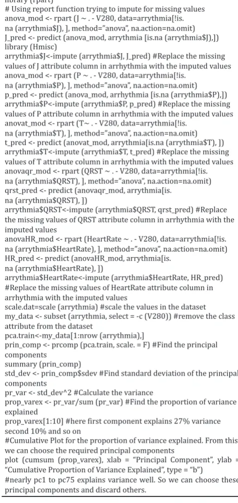
library (rpart)
# Using report function trying to impute for missing values anova_mod <- rpart (J ~ . - V280, data=arrythmia[!is. na (arrythmia$J), ], method=”anova”, na.action=na.omit) J_pred <- predict (anova_mod, arrythmia [is.na (arrythmia$J),]) library (Hmisc)
arrythmia$J<-impute (arrythmia$J, J_pred) #Replace the missing values of J attribute column in arrhythmia with the imputed values anova_mod <- rpart (P ~ . - V280, data=arrythmia[!is.
na (arrythmia$P), ], method=”anova”, na.action=na.omit) p_pred <- predict (anova_mod, arrhythmia [is.na (arrythmia$P),]) arrythmia$P<-impute (arrythmia$P, p_pred) #Replace the missing values of P attribute column in arrhythmia with the imputed values anovat_mod <- rpart (T~ . - V280, data=arrythmia[!is.
na (arrythmia$T), ], method=”anova”, na.action=na.omit) t_pred <- predict (anovat_mod, arrythmia[is.na (arrythmia$T), ]) arrythmia$T<-impute (arrythmia$T, t_pred) #Replace the missing values of T attribute column in arrhythmia with the imputed values anovaqr_mod <- rpart (QRST ~ . - V280, data=arrythmia[!is. na (arrythmia$QRST), ], method=”anova”, na.action=na.omit) qrst_pred <- predict (anovaqr_mod, arrythmia[is.
na (arrythmia$QRST), ])
arrythmia$QRST<-impute (arrythmia$QRST, qrst_pred) #Replace the missing values of QRST attribute column in arrhythmia with the imputed values
anovaHR_mod <- rpart (HeartRate ~ . - V280, data=arrythmia[!is. na (arrythmia$HeartRate), ], method=”anova”, na.action=na.omit) HR_pred <- predict (anovaHR_mod, arrythmia[is.
na (arrythmia$HeartRate), ])
arrythmia$HeartRate<-impute (arrythmia$HeartRate, HR_pred) #Replace the missing values of HeartRate attribute column in arrhythmia with the imputed values
scale.dat=scale (arrythmia) #scale the values in the dataset my_data <- subset (arrythmia, select = -c (V280)) #remove the class attribute from the dataset
pca.train<-my_data[1:nrow (arrythmia),]
prin_comp <- prcomp (pca.train, scale. = F) #Find the principal components
summary (prin_comp)
std_dev <- prin_comp$sdev #Find standard deviation of the principal components
pr_var <- std_dev^2 #Calculate the variance
prop_varex <- pr_var/sum (pr_var) #Find the proportion of variance explained
prop_varex[1:10] #here first component explains 27% variance second 10% and so on
#Cumulative Plot for the proportion of variance explained. From this we can choose the required principal components
plot (cumsum (prop_varex), xlab = “Principal Component”, ylab = “Cumulative Proportion of Variance Explained”, type = “b”)
#nearly pc1 to pc75 explains variance well. So we can choose these principal components and discard others.
Table 4: Feature vector corresponding to first two eigen values
X1 X2
0.36138659 −0.65658877
−0.08452251 −0.73016143
0.85667061 0.17337266
0.35828920 0.07548102
Table 6: Sample of the final reduced dataset with just two columns
X1 X2
−2.684126 −0.3193972
−2.714142 0.1770012
−2.888991 0.1449494
−2.745343 0.3182990
−2.728717 −0.3267545
−2.280860 −0.7413304
Table 5: Transpose of the feature vector Feature_
vectors [1] [2] [3] [4]
X1 0.361386 −0.08452251 0.8566706 0.35828920
X2 −0.656588 −0.73016143 0.1733727 0.07548102
Proportion of variance explained for first 10 principal components 0.27512611, 0.10787279, 0.07843598, 0.06887855, 0.06004577, 0.04251144, 0.03758893, 0.03160052, 0.02903681, 0.02415692. The first principal component captures 27% of variance from the whole dataset, second principal component captures 10.7% and so on.
From the Fig. 1 we are able to understand that the first 75 principal components are able to capture most of the variance from the whole dataset. Hence we can choose these 75 principal components as the reduced dimensions from the whole data of 279 attributes.
CONCLUSION
In this survey, four different dimensionality reduction techniques have been studied. The selection of dimensionality reduction technique is based on the scenario, for example, the nature of the dataset that has to be reduced. The dimensionality reduction techniques are been performed to reduce the time elapsed in processing high-dimensional data, improve accuracy and efficiency in the analysis. An experiment that demonstrates the PCA method and how it helps in performing dimensionality reduction of data has been explained.
In future, the implementation of each of these methods in large dataset can be performed and these techniques can be analyzed based on time, accuracy in prediction and their efficiency. The implementation of such techniques in health care datasets would be highly helpful for early diagnosis or prediction of diseases in a much lesser time with high accuracy.
REFERENCES
1. Chen XW, Lin X. Big data deep learning: Challenges and perspectives. IEEE Access 2014;2:514-25.
2. Chen HL, Yang B, Liu J, Liu DY. A support vector machine classifier with rough set-based feature selection for breast cancer diagnosis. Expert Syst Appl 2011;38(7):9014-22.
3. Bae JH, Jeon YJ, Lee S, Kim JU. A feasibility study on age-related factors of wrist pulse using principal component analysis. In: Engineering in Medicine and Biology Society (EMBC), IEEE
38th Annual International Conference; 2016. p. 6202-5.
4. Seng KP, Ang LM, Ooi CS. A combined rule-based & machine learning audiovisual emotion recognition approach. IEEE Trans Affect Comput 2016;12:1-11.
5. Fuadi T, Bustami A, Umran YM. Singular Value Decomposition for Dimensionality Reduction in Unsupervised Text Learning Problems,
2nd International Conference on Education Technology and Computer
(ICETC). Vol. 4. 2010. p. 4-422.
6. Ibrahim AO, Shamsuddin SM, Saleh AY, Abdelmaboud A, Ali A. Intelligent multi-objective classifier for breast cancer diagnosis based on multilayer perceptron neural network and differential evolution. In: Computing, Control, Networking, Electronics and Embedded Systems Engineering (ICCNEEE), International Conference; 2015. p. 422-7. 7. Berral-García JL. A quick view on current techniques and machine
learning algorithms for big data analytics. In: Transparent Optical
Networks (ICTON), 18th International Conference; 2016. p. 1-4.
8. Tang X, Wu J. Principal component analysis of the shape deformations of the hippocampus in Alzheimer’s disease. In: Engineering in
Medicine and Biology Society (EMBC), IEEE 38th Annual International
Conference; 2016. p. 4013-6.
9. Li LN, Ouyang JH, Chen HL, Liu DY. A computer aided diagnosis system for thyroid disease using extreme learning machine. J Med Syst 2012;36(5):3327-37.
10. Zhao R, Mao K. Semi-random projection for dimensionality reduction and extreme learning machine in high-dimensional space. IEEE Comput Intell Mag 2015;10(3):30-41.
11. Snehal KJ, Machchhar S. An Evolution and Evaluation of Dimensionality Reduction Techniques - A Comparative Study. IEEE International Conference on Computational Intelligence and Computing Research; 2014.
12. Wei C, Chen J, Song Z. Nonlinear Process Monitoring Using Improved
Kernel Principal Component Analysis, IEEE 28th Chinese Control and
Decision Conference (CCDC); 2016. p. 5838-43.
13. Iosifidis A, Gabbouj M. Combining multi-class maximum margin classification with linear discriminant analysis for human action recognition. In: Image Processing (ICIP), IEEE International Conference; 2016. p. 4180-4.
14. Khodr J, Younes R. Dimensionality reduction on hyperspectral images: A comparative review based on artificial datas. In: Image and Signal