Article
1
Utilizing UAV and 3D Computer Vision for Visual Inspection of a
2
Large Gravity Dam
3
Ali Khaloo 1, David Lattanzi 1,* and Adam Jachimowicz 2
4
1 Department of Civil, Environmental, and Infrastructure Engineering, George Mason University, Fairfax,
5
VA, USA, 22030; [email protected] (A.K.); [email protected] (D.L.)
6
2 Argonne National Laboratory, Washington, D.C., USA, 20024; [email protected]
7
* Correspondence: [email protected]; Tel.: +1-703-993-3695
8
9
Abstract: Dams are a critical infrastructure system for many communities, but they are also one of
10
the most challenging to inspect. Dams are typically very large and complex structures, and the result
11
is that inspections are often time-intensive and require expensive, specialized equipment and
12
training to provide inspectors with comprehensive access to the structure. The scale and nature of
13
dam inspections also introduces additional safety risks to the inspectors. Unmanned aerial vehicles
14
(UAV) have the potential to address many of these challenges, particularly when used as a data
15
acquisition platform for photogrammetric three-dimensional (3D) reconstruction and analysis,
16
though the nature of both UAV and modern photogrammetric methods necessitates careful
17
planning and coordination for integration. This paper presents a case study on one such integration
18
at the Brighton Dam, a large-scale concrete gravity dam in Maryland, USA. A combination of
19
multiple UAV platforms and multi-scale photogrammetry was used to create two comprehensive
20
and high-resolution 3D point clouds of the dam and surrounding environment at intervals. These
21
models were then assessed for their overall quality, as well as their ability to resolve flaws and
22
defects that were artificially applied to the structure between inspection intervals. The results
23
indicate that the integrated process is capable of generating models that accurately render a variety
24
of defect types with sub-millimeter accuracy. Recommendations for mission planning and imaging
25
specifications are provided as well.
26
Keywords: Infrastructure Inspection; Computer Vision; Structure from Motion; Dam Inspection; 3D
27
Scene Reconstruction; Aerial Robots; Remote Sensing; Structural Health Monitoring; Unmanned
28
Aerial Vehicles
29
30
1. Introduction
31
Dams are critical infrastructure systems for many communities, but they are also one of the most
32
challenging to inspect due to their complex nature. Dams can experience a range of problems during
33
their service life, and improper operation and maintenance result in major issues. Furthermore, dams
34
can be deteriorated due to weathering, alkali-aggregate reaction (AAR, or alkali-silica reaction, ASR),
35
freezing and thawing, or other chemical reactions. The Federal Emergency Management Agency
36
(FEMA) publishes the Guidelines for Dam Safety [1], and suggest that formal inspections occur at
37
least every 5 years. They also recommend informal, intermediate and special inspections as needed.
38
The Maryland Department of Environment also recommends that owners inspect their dams after
39
extreme rainfall and formally once every 5 years [2]. According to the American Society of Civil
40
Engineers’ (ASCE) 2017 Infrastructure Report Card [3] the average age of the 90,580 dams in the
41
United States is 56 years, with 17% rated as high-hazard potential dams necessitating additional
42
inspections.
43
The conventional standard of practice requires a detailed visual inspection not just of the
44
primary structure, but of the subsystems and the surrounding watershed as well. Dams are typically
45
very large and complex structures, and consequently dam inspections are time-intensive and require
46
expensive, specialized equipment and training to provide inspectors with comprehensive access to
47
the structure. The scale and nature of dam inspections also introduces additional safety risks to the
48
inspectors. Typically, a limited number of photographs, and occasionally videos, are captured to
49
provide a visual record of the current state of the structure. By themselves, these recordings are not
50
ideal data products, as reviewing them can be tedious and the lack of spatial context can prove
51
disorienting to data analysts and engineers.
52
Recently, there have been advancements in the use of 3D imaging systems for capturing the
in-53
situ 3D state of civil infrastructure systems [4]. The most widely used technology for generating 3D
54
models, or point clouds, is Terrestrial Laser Scanning (TLS). A lower-cost alternative and somewhat
55
complimentary approach is to use photogrammetric methods to extract 3D geometries from large
56
sets of two-dimensional (2D) digital images. In either case, the result is a scale-accurate,
high-57
resolution virtual model of a structure and its surrounding areas. These digital models capture
58
current conditions of the entire structure that can be used for archival and analytical purposes [4, 5].
59
However, both 3D imaging approaches suffer from the same access challenges that hinder
60
conventional visual inspections.
61
Unmanned aerial vehicles (UAV) are a disruptive innovation [6] with potential to transform
62
traditional dam inspection methodologies by expanding the capabilities of 3D imaging in these
63
environments. While UAV have been in use for some time, their recent popularity is in part due to
64
reductions in hardware costs, improvements to software interfaces, and to the expanded range of
65
sensor payload options [7]. The portability, mobility, and low cost of UAV can mitigate the need for
66
expensive inspection access equipment and reduce safety risks to inspectors [8]. Furthermore, UAV
67
serve as an almost ideal data collection platform for modern 3D reconstruction techniques. Critically,
68
the nature of both UAV and 3D reconstruction methods necessitate careful planning and coordination
69
to properly integrate and tailor these technologies for dam inspection.
70
1.1. Prior Work on Modern Dam Inspection
71
The reduced accessibility of dams, both for uptake needs and for their strategic nature, and the
72
large amount of time needed for an inspection by traditional methods do not facilitate direct visual
73
inspection. Therefore, novel methods that integrate modern remote sensing tools, robotics and
74
computer vision techniques have been investigated in the past few years. In the work by Ridao et al.
75
[9], an Autonomous Underwater Vehicle (AUV) was designed to collect images from a hydroelectric
76
dam which was later used to generate photomosaic (with approximate resolution of 1 pixel/mm) of
77
the inspected area to help with the visual inspection. González-Aguilera et al. [10] studied the
78
viability of utilizing TLS systems to generate 3D models of a large concrete dam and further assessed
79
its capability for structural monitoring. However, due to the limited access for data acquisition, the
80
final model lacked the necessary completeness to capture the entire dam. Berberan et al. [11] studied
81
using TLS for deformation monitoring of the downstream face of the Cabril Dam in Portugal using
82
3D models generated at two different times for comparison purposes. Although both of the
83
aforementioned studies proved the value of 3D modeling using TLS for dam inspection, they were
84
not able to capture the overall geometry and resolve the fine-scale (1mm) details needed for accurate
85
visual inspection.
86
In the study by González-Jorge et al. [12], photogrammetric 3D modeling using UAV acquired
87
imagery was tested for the monitoring of dam breakwaters. Recently, researchers have focused on
88
using camera-equipped UAV to facilitate dam visual inspection through 3D modeling [13, 14].
89
Although using UAV provided unprecedented access to different parts of the dam at a lower cost,
90
the complex geometry and large size of these structures made it impossible to reconstruct a complete
91
model of the targeted structures.
92
In the recent work by Buffi et al. [15], UAV-based photogrammetry was used as a new tool for
93
surveyors to generate a complete 3D model of the Rideacoli Dam in Italy. The generated model was
94
compared against conventional techniques such as total stations, TLS and Global Positioning System
95
(GPS) to assess the overall geometry captured through 3D photogrammetric approach. The
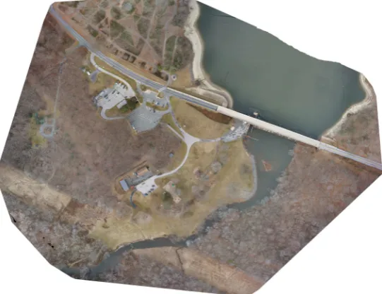
96
of the model was estimated to be an average of one point every 1 cm2 which may be inadequate for
98
detailed visual inspection of smaller scale damages such as cracks.
99
1.2. Contributions of This Work
100
This paper presents a case study on integrating aerial robots and 3D computer vision for visual
101
inspection of a large gravity dam in the United States. A combination of multiple UAV platforms and
102
photogrammetric approaches was used to create two comprehensive 3D point clouds of a dam and
103
surrounding environment that were then assessed for their relative quality and ability to render
104
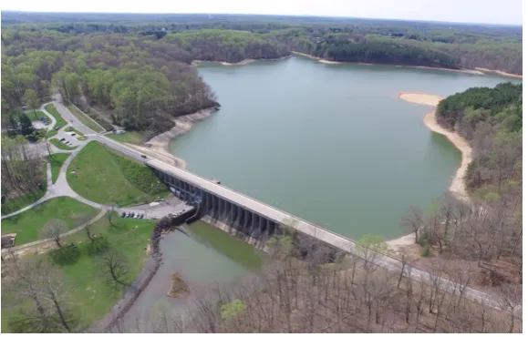
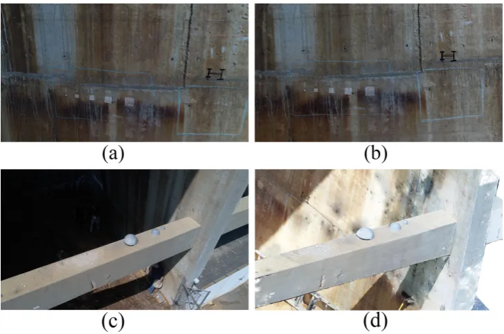
artificially applied defects. The Brighton Dam, located in Brookeville, Maryland and managed by the
105
Washington Suburban Sanitary Commission (WSSC), was selected as the subject of this study (Figure
106
1). The dam was put into service in 1944, and is representative of a large-scale gravity dam in-service
107
across the United States.
108
109
Figure 1. The Brighton Dam.
110
The key technical contributions of this work include the development and assessment of a
multi-111
UAV system for generating massive, dense, and comprehensive 3D point clouds (contain more than
112
one billion points) of the targeted dam system, as well as an evaluation of the imaging specifications
113
necessary to render small-scale inspection details. It is also the first time, to the authors’ best
114
knowledge, that a multi-scale photogrammetric 3D reconstruction technique has been used to
115
capture the overall geometry of a large-scale complex gravity dam while simultaneously resolving
116
structural flaws on the order of 1 mm using UAV-acquired images.
117
The details of the data collection procedure are presented first, followed by reporting of the
118
operations on two inspection mission days. This is followed by a presentation of the data processing
119
and analysis methodologies. An evaluation of the results of the methodological approach for the
120
Brighton Dam inspection is included as well. The paper concludes with a summation of the findings
121
of the research team and avenues for future work in this domain.
122
2. Data Collection
123
2.1. Logistics and Planning
124
The goal of the field testing was to collect two comprehensive sets of digital images to be
125
converted into 3D point clouds, using a combination of DSfM and rigid registration techniques. The
126
point clouds needed to have the point density—analogous to resolution—necessary to resolve
127
inspection details on the millimeter scale while comprehensively capturing the overall spatial
128
context of the dam. To achieve this, image acquisition in terms of camera positioning, the number of
129
A variant of the DSfM process previously developed by the research team was chosen to
131
generate 3D point clouds [8, 16]. This process, referred to as Hierarchical Point Cloud Generation
132
(HPCG), is designed to integrate images captured at a wide range of standoff distances from a
133
structure into one complete model. From a data collection standpoint, images are collected in networks
134
of similar standoff distances. The images from each network are then integrated and merged into a
135
global, multi-scale point cloud model, as presented in the later sections of the paper.
136
Both fixed-wing and multi-rotor UAV platforms with mounted cameras were used to acquire
137
image networks. The concept was to use the fixed wing UAV to capture the global geometry of
138
both the upstream and downstream faces of the dam, and for the multi-rotor UAV to generate
139
a series of oblique image networks from varying standoff distances. UAV flight planning that
140
resulted in images with greater than 80% overlap between adjacent photos was desired to minimize
141
the ground sample distance (GSD) and consequently maximize the spatial resolution. The minimum
142
standoff distance from the dam was held to approximately 2.5m. This corresponded to a pixel size of
143
approximately 0.0024 (mm/pixel) and a GSD of 0.6 mm in the plane of the dam façade for the lowest
144
resolution sensor used during the project.
145
These images networks were collected over the course of two distinct days, in order to simulate
146
variances in field conditions between inspection intervals and provide a basis for temporal analysis
147
between the subsequent models. Data collection on the first day was designed to comprehensively
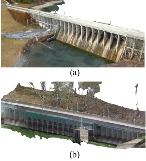
148
image the entire dam and environs using a combination of three different UAV. Data collection on
149
the second day focused on an isolated section of the dam that was selected for the defect analysis
150
portion of the study, as will be discussed later.
151
A custom-built fixed wing mounted with a Sony Alpha Series 5100 camera (24.3-megapixels)
152
with a Sony E-PZ 16–50 mm lens was used to capture a series of nadir angle shots that covered the
153
dam and the surrounding area. The utilized UAV’s airframe was the Super Sky Surfer fixed wing
154
expanded polyolefin (EPO) foam frame. It was modified in order to custom fit various components,
155
such as the autopilot, GPS module, airspeed sensor, camera payload, motor and batteries. The
156
communication between the UAV and ground control station (GCS) was done through radio
157
telemetry.
158
Two DJI Inspire 1 aircrafts mounted with 12-megapixel (MP) cameras were used to separately
159
capture oblique imagery of the downstream and upstream portions of the dam. On the second day
160
of data collection, in addition to capturing the entire dam structure, the mission was to focus on a
161
specific region of the dam, Bay #5 of the downstream façade with preinstalled targets, which required
162
maneuvering a UAV in a confined space. For this task, a DJI Phantom 4 Pro with a 16-MP camera, a
163
smaller quadcopter aircraft, was selected due to its better maneuverability and collision avoidance
164
features relative to the other available aircraft.
165
The logistics of flying multiple UAV over the two mission days, along with the complexities of
166
the dam environment, meant that proper planning was essential. After the UAV pilots confirmed the
167
test site was not in a restricted airspace, and that safe operations were feasible, the team began to
168
target dates for data collection.
169
The performance of UAV inspection imaging is primarily dependent on operating conditions
170
that do not impede piloting of the UAV itself. In particular, cold weather was a key consideration
171
when identifying mission dates. The team determined that the battery life of the selected UAV would
172
not operate sufficiently in temperatures below 5 degrees Celsius. Rain, snow, and high winds were
173
also weather phenomena that dictated the ability to operate the UAV safely. Secondary to selecting
174
mission days with viable UAV operating conditions, radiometric conditions that optimized the
175
consistency of UAV imagery were preferred. High contrast lighting, typically due to bright sun
176
conditions, can create strong shadows that degrade the performance of the DSfM process [8, 17].
177
2.2. Day One Operation
178
Mission planner software was used to develop a flight plan for the fixed wing nadir imaging
179
that would allow the aircraft and camera to operate autonomously. A lawnmower pattern for an area
180
1.69 seconds/image was specified, resulting in 558 nadir images (Figure 3). Total flight time for the
182
fixed wing UAV was 26 minutes.
183
184
Figure 2. Flight path for fixed wing UAV.
185
The two rotary UAV were piloted manually, with a second operator controlling the camera and
186
gimbal in order to guarantee the specified 80% overlap between images and maintain standoff
187
distances, specified to maximize the quality of the DSfM reconstructions. In total 2020 images of the
188
structure were captured using all three aircrafts.
189
190
Figure 3. Orthomosaic generated using the fixed wing imagery dataset.
191
2.3. Day Two Operation
192
The second day of operations also focused on Bay #5, on the downstream face of the dam. The
193
goals of this day’s operations were to generate a point cloud for comparisons with the point cloud
194
generated through Day One operations, as well as to assess the quality of the UAV point cloud
195
generation process for resolving small-scale structural defects.
196
Prior to UAV flight and imaging inside Bay #5, a series of controlled and simulated defects with
197
known dimensions were applied to the dam structure, serving as a benchmark for reconstruction
198
accuracy and analytical testing. Overall, three different types of defects were applied: linear markings
199
with controlled thickness (Type 1), square surface area markings (Type 2), and spherical volumes
200
Type 1 defects were designed to simulate cracking and crack-like defects. Line thicknesses of
202
0.7mm, 1mm, and 3mm widths were applied, with lines varying in length from 12.7 mm to 152.4 mm
203
for each width. The sets of lines were applied using both black and white chalk on the sides of Bay
204
#5 (Figure 4). Type 2 defects were designed to simulate localized area defects such as concrete efflorescence, or
205
staining due to corrosion. These defects took the form of a series of square chalk markings (Figure 4) with
206
dimensions varying from 645 mm2 to 16129 mm2. Type 3 defects simulated volumetric changes, such
207
as concrete spall off. As physically removing portions of the dam structure was not permissible,
208
volumes were instead temporarily added to the structure. Three Styrofoam hemispheres, with
209
diameters of 127 mm, 203.2 mm and 304.8 mm (Figure 4) were painted and textured to have the visual
210
appearance of concrete, and placed on the lateral brace of Bay #5.
211
212
Figure 4. Controlled simulated damages: (a) 2D image of Type 1 and 2 defects; (b) 3D point cloud
213
rendering of Type 1 and 2 defects; (c) 2D image of Type 3 volumetric defects; (d) 3D point cloud
214
rendering of Type 3 volumetric defects.
215
2.4. Laser Scanning
216
For comparative purposes, a phase-shift based Faro Focus3D laser scanner was used to collect
217
data from downstream face of the dam. The quality of the data collection was set to 6x in order to
218
reduce the noise in the scan data and thus increases the scan quality. Due to placement limitations, it
219
was not possible to capture the upstream face of the dam with the scanner. A total of 9 scans was
220
collected and merged using the Faro SCENE software.
221
3. 3D Point Cloud Generation
222
From the available algorithms for image-based 3D reconstruction techniques, in this work a variant of
223
the Structure-from-Motion (SfM) process was chosen. SfM is based on the simultaneous recovery of both
224
the 3D geometry (structure) of a scene and the camera pose (motion) using a sparse set of
225
correspondences between image features, and has been shown to produce results comparable to laser
226
scanners [17, 19].
227
The first step in the SfM process is to automatically detect keypoint feature descriptors (pixel
228
locations that are highly distinctive) such as the Scale Invariant Feature Transform (SIFT) [20] in each
229
input image. Next, feature descriptors are matched between pairs of images by finding a
230
correspondence in the second image using a nearest neighbor similarity search [21] to construct the
231
relationship of feature points between image pairs, called tracks.
Because corresponding points in two images are subject to the epipolar constraints (describe by
233
the fundamental matrix), filtering the matches by enforcing these constraints removes false
234
correspondences [18]. By using the normalized eight-point algorithm [22] in tandem with the
235
RANSAC (RANdom SAmple Consensus) [23] paradigm, it is possible to minimize the number of
236
wrong matches across images.
237
Next, an initial image pair with a large number of matched features and a long separation
238
distance is selected and their camera parameters are estimated using the 5-point algorithm [24],
239
followed by triangulation of the matched features using the polynomial method [25]. Subsequently,
240
new images are added by using the correspondences between 3D points and image features through
241
the Perspective n-Point (PnP) algorithm with RANSAC and Gauss-Newton optimization [26].
242
After the orientation of each image, bundle adjustment (a nonlinear least-squares problem) is
243
performed to minimize the sum of re-projection errors using the Levenberg-Marquardt algorithm [27].
244
In this process intrinsic camera parameters matrix, K, along with the pose of each particular camera
245
described by rotation, R, and the position of its optical center, C, as well as the positions of the 3D
246
points X are optimized simultaneously.
247
− − → min
, , ,
∈ (1)
Where ∈ indicates that the point Xi is visible in image j, and xijdenotes the projection of 3D
248
points Xi onto image j. This procedure is repeated until an orientation is available for all images
249
within each imaging network. The result of this pipeline is a relatively sparse set of 3D points, due to
250
only utilizing extracted feature points in the 3D reconstruction.
251
In order to densify the reconstructed models and produce a model dense enough to capture
252
small geometric changes, multi-view stereo algorithms [17] are used to capture information from all
253
pixels in the input 2D images. In this work, the Semi-Global Matching (SGM) algorithm [28] was used
254
to perform pairwise dense matching, as it has been shown to provide a high level of point density
255
relative to other methods utilized for densification [16, 17]. The SGM algorithm uses a pixel-wise
256
matching cost for compensating radiometric differences of registered images within the depth map
257
estimation. Later, individual depth maps are merged together through depth map fusion techniqueto
258
generate a single, globally consistent 3D representation [29].
259
The HPCG approach used in this study is designed for seamlessly matching and integrating
260
images with different scales, viewpoints, and cameras into one single reconstruction [16]. The HPCG
261
process begins by first generating 3D point clouds separately for each image network, using the
262
aforementioned photogrammetric process. The point clouds generated for each network are then
263
merged together into a single model using the Iterative Closest Point (ICP) algorithm [30]. The ICP
264
approach refines the alignment assuming an initial coarse registration of the 3D models is provided.
265
This initial alignment can be performed through pair-wise matching of 10 manually selected point
266
correspondences in order to reduce the inherent sensitivity of the ICP algorithm regarding the initial
267
positions of the 3D models.
268
The rigid transformation between two sets of corresponding 3D point sets = { , , ⋯ , } and
269
= { , , … , } extracted through utilizing kd-trees [21], can be formulated as the solution of the
270
least-squares problem:
271
( , ) = argmin
, ‖( + ) − ‖ (2)
Where rotation matrix R and translation vector t can be derived by arranging the point in two
272
3×N matrices and that have ̅ and as columns:
273
̅ = − ∑ , = − ∑ (3)
By computing the Singular Value Decomposition (SVD) of the 3×3 covariance matrix ,
274
∑ = ( ), the optimal R and t are given by:
= 1 1
det( ) , = ∑ − ∑ (4)
These rotations and translations are then used to align the individual point clouds for each
276
network and form the complete global model. The result is a multi-scale/resolution 3D model that
277
allows for higher resolution and emphasis in critical regions of structures. This approach also
278
increases the rate of image registration during the SfM process, thereby improving model accuracy,
279
resolution and completeness.
280
3.1. Brighton Dam Model Generation
281
For this process to work properly there must be a global point cloud that captures the overall
282
geometry of the structure, and into which the other point clouds are merged through ICP. In this
283
work, this geometry network was captured using the fixed wing UAV. The second key criterion is
284
that the standoff distances between merged point clouds cannot vary excessively. This was
285
accomplished by capturing images at varying standoff distances (range from 2.5 m to 10 m).
286
4. Case Study Results
287
The images collected on Day One and processed using the HPCG technique yielded a point
288
cloud of 1,469,690,005 points (Figure 5). The Day Two mission resulted in a model with 997,799,119
289
points.
290
291
Figure 5. Generated 3D Point cloud of the Brighton Dam: (a) Downstream face; (b) Upstream face.
292
4.1. Point Cloud Quality Analysis
293
Three metrics were used to assess the point clouds: (i) local noise level, (ii) local point density,
294
The noise level in a point cloud is defined as the residual between each point and the best fitting
296
plane computed on its local nearest neighbours. Digital image noise, radiometric parameters,
297
nonconformity of the neighbourhood of a point, imperfect data registration, and DSfM reconstruction
298
inaccuracies can all affect this characteristic.
299
This noise residual is defined as the lowest valued eigenvalue of the covariance matrix for a local
300
neighborhood around a point in a cloud. For the k points that form the neighborhood of a 3D point pi
301
in a point cloud, the 3×3 covariance matrix, C, is defined as [31]:
302
= ∑ ( − ̅)( − ̅) ; ̅ = ∑ (5)
Where ̅ is the arithmetic mean within pi’s neighbourhood (Npi) and C represents a symmetric
303
positive-definite matrix. By performing SVD on the covariance matrix, it is possible to compute
304
eigenvectors V (v2, v1, and v0) and their corresponding eigenvalues ≥ ≥ ≥ 0. Within this
305
approach, v0 approximates the point’s pi normal, while quantitatively describes the variation
306
along the normal vector to provide an estimation of the local noise level (i.e. roughness). In addition,
307
the normalized surface variation or curvature ( ) can be defined as , which is invariant under
308
rescaling [32]. For this study a value of k=30 points was empirically specified for roughness
309
calculations (Figure 6).
310
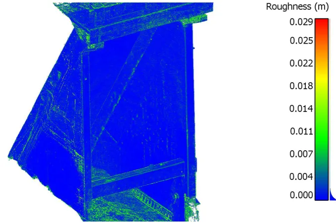
311
Figure 6. Estimated noise level (lowest eigenvalue λ0) for Bay#5; low to high noise level ranges from
312
dark to light intensity.
313
The second metric, local point density, is a characteristic analogous to pixel resolution in 2D
314
digital images. It corresponds to the ability of a 3D point cloud to resolve structural defects and
small-315
scale details. It also provides insight in the variations in point cloud quality that stem from the
multi-316
UAV imaging approach. The local density at a point pi is defined as = , where rk-NN is
317
the radius of the spherical neighbourhood of the k closest neighbours of a 3D point. In this study, r
k-318
NN was set to 0.62 centimeters to achieve an enclosing volume of 1 cm3.
319
The last evaluative metric was to measure the defects applied to Bay #5 during the second
320
mission day, in the resulting 3D point cloud. Both Type 1 and 2 simulated damages were manually
321
measured from the point cloud models and the results was compared against the field measurements.
322
In order to lessen the error, each manual pairwise point selection and its subsequent Euclidean
323
distance measurement was repeated 10 times and their average value was compared against the
324
ground-truth values measured in the field.
325
Volumetric defects (Type 3) were measured by using the direct cloud-to-cloud (C2C) distance
326
point clouds. Upon finding the closest point correspondences in the two registered clouds, the
328
Hausdorff distance was utilized to find the distance between points in the first dataset and their
329
closest points in the second dataset. Given two finite point sets = { , , ⋯ , } and =
330
{ , , … , }, the two-sided Hausdorff distance H(P, Q) is defined as:
331
( , ) = max(max
∈ min∈ ‖ − ‖, max∈ min∈ ‖ − ‖) (6)
Note that this notation of distance is purely geometric and does not make any assumptions on
332
the uniformity of the point cloud density. Using this method provided the radius of each hemisphere,
333
which was later used to estimate their volume.
334
4.2. Point Cloud Analysis Results
335
The results of the point cloud quality analysis are shown in Table 1. Model density from the
336
January UAV flights was substantially higher than those generated through TLS or during the April
337
flights. The differences between the two HPCG models is likely due to the change in sensor resolution
338
between mission days and changes in the flight protocols, as the April flights focused on Bay #5.
339
Average roughness and curvature values for the three models are all of a similar order of magnitude,
340
indicating relatively similar 3D geometric accuracy. As can be seen, the point cloud generated by the
341
laser scanner consists of significantly fewer points than the models generated through HPCG. This
342
was due to the limited options for scanner placement, particularly with respect to the higher elevation
343
regions of the dam façade and the upstream façade. Point cloud quality analysis for the Bay #5 region
344
of the dam are shown in Figure 7 and Table 2.
345
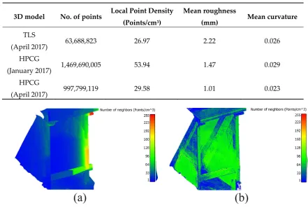
Table 1. Point Cloud Quality Analysis.
346
3D model No. of points Local Point Density (Points/cm3)
Mean roughness
(mm) Mean curvature
TLS
(April 2017) 63,688,823 26.97 2.22 0.026
HPCG
(January 2017) 1,469,690,005 53.94 1.47 0.029
HPCG
(April 2017) 997,799,119 29.58 1.01 0.023
347
Figure 7. Local point density for Bay#5; low to high density ranges from dark to light intensity: (a)
348
Day One dataset; (b) Day Two dataset.
349
These results highlight the advantages of using a UAV for point cloud generation. Both HPCG
350
models had over twice the density and mean roughness values less than half those of the laser
351
scanner. These performance improvements can be attributed to the ability of the UAV to capture
352
those areas from the ground. Compared to the overall point cloud models, the results for the HPCG
354
models are more similar for Bay #5.
355
Table 2. Point Cloud Quality Analysis for Bay #5.
356
3D model No. of points Local Point Density (Points/cm3)
Mean roughness
(mm)
Mean
curvature
TLS
(April 2017) 28,356,650 20.81 2.21 0.036
HPCG
(January 2017) 108,286,272 56.19 0.92 0.026
HPCG
(April 2017) 159,579,984 69.31 0.58 0.018
In order to assess how image resolution affected model quality, the images captured via UAV
357
during the April mission were downsampled to 50%, 25%, and 12.5% of the original image size using
358
the bicubic image interpolation. The downsampled images were then used to regenerate point clouds
359
of Bay #5. The resulting model assessments are shown in Table 3.
360
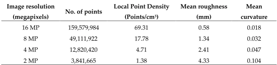
Table 3. Bay #5 3D Point Cloud Generation using Various Image Resolutions.
361
Image resolution
(megapixels) No. of points
Local Point Density
(Points/cm3)
Mean roughness
(mm)
Mean
curvature
16 MP 159,579,984 69.31 0.58 0.018
8 MP 49,111,922 17.78 1.34 0.032
4 MP 12,820,420 4.71 2.41 0.047
2 MP 3,841,665 1.38 4.33 0.104
With a loss of image resolution, the density of the models is reduced, as expected. This reduction
362
does not scale linearly with the number of pixels, but quadratically. Notably, the average cloud
363
roughness increases with a reduction in image resolution, as can be seen in the images disparity maps
364
(Figure 8). This suggests that the reduced number of feature points used for SfM reconstruction along
365
with excessive noise within the depth map estimation and fusion (Figure 8) affected the accuracy and
366
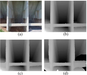
368
Figure 8. (a) Original input image; (b) depth map reconstructed for the 16 MP image; (c) depth map
369
reconstructed for the 8 MP image; (d) depth map reconstructed for the 2 MP image. Each depth
370
value encodes the distance from the camera center to the geometry.
371
4.3. Evaluation of Flaw Resolving Capabilities
372
Tables 4 and 5 summarize the comparisons between the ground-truth dimensions of the Type 1
373
defects and the dimensions measured in the point cloud. For the 1mm and 3mm defect widths, the
374
point clouds generated using 16 MP images were able to resolve all of the flaws to a degree that
375
highly accurate measurements were possible. However, as image resolution decreased, measurement
376
accuracy decreased. For models using 4 MP or less in resolution, most flaws were not resolved at all
377
in the models and so measurements were not possible. None of the models were able to reconstruct
378
the 0.7mm flaws.
379
Table 4. Measurement Accuracy of 1 Millimeter Type 1 Defects at Various Image Resolutions.
380
Ground truth defect length
(mm)
Length measured in point cloud (mm)
16 MP 8 MP 4 MP 2 MP
12.7 13 - - -
25.4 27.0 23 - -
76.2 73 72 - -
152.4 150.2 142 - -
These results suggest that a point density somewhere between 18 points/m3 and 69 points/m3
381
was necessary to guarantee the reconstruction of Type 1 flaws in the model. During these tests, the
382
image resolution and the sensor dimensions of the DJI Phantom 4 camera, each pixel in the images
384
corresponded to approximately 1mm in the plane of the defects.
385
Table 5. Measurement Accuracy of 3 Millimeter Type 1 Defects at Various Image Resolutions.
386
Ground truth defect length
(mm)
Length measured in point cloud (mm)
16 MP 8 MP 4 MP 2 MP
12.7 13 10 - -
25.4 26 25 - -
76.2 76 72 68 -
152.4 151 152 139 -
The measurements for Type 2 defects are shown in Table 6. For these defects, the models derived
387
from either the 16 MP (69 points/m3) or the 8 MP (18 points/m3) images were able to accurately resolve
388
the flaws. However the 4 MP and 2 MP image models were not able to consistently resolve defects.
389
This corresponds to a minimum pixel size of 1.5 mm in the plane of the defect.
390
Table 6. Measurement Accuracy of Type 2 Defects at Various Image Resolutions.
391
Ground truth defect size
(mm × mm)
Size measured in point cloud (mm × mm)
16 MP 8 MP 4 MP 2 MP
25.4 × 25.4 26 × 25 26 × 24 - -
50.8 × 50.8 51 × 50 52 × 51 - -
76.2 × 76.2 76 × 76 76 × 76 62 × 70 -
101.6 × 101.6 100 × 100 97 × 100 98 × 93 -
127 × 127 127 × 127 125 × 125 121 × 125 -
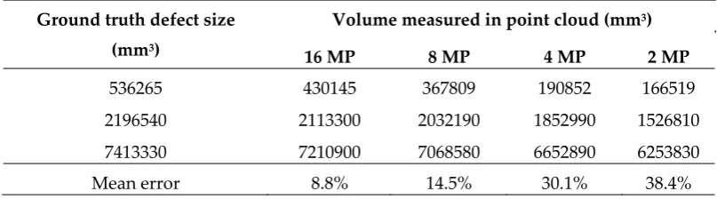
The measurement results for the Type 3 volumetric defects are shown in Figure 9 and Table 7.
392
For this test, all levels of image resolution were able to generate models that captured all three
393
volumetric changes. However, the reduction in image resolution resulted in systematic under
394
prediction of volume measurements.
395
396
Figure 9. Volumetric 3D change analysis.
397
Table 7. Measurement Accuracy of Type 3 Volumetric Defects at Various Image Resolutions.
399
Ground truth defect size
(mm3)
Volume measured in point cloud (mm3)
16 MP 8 MP 4 MP 2 MP
536265 430145 367809 190852 166519
2196540 2113300 2032190 1852990 1526810
7413330 7210900 7068580 6652890 6253830
Mean error 8.8% 14.5% 30.1% 38.4%
4.4. Limitations and Sources of Error
400
The process used to generate the point clouds has two key sources of error. The first is
401
misalignment of cameras at the image matching stage. The second is misalignment of individual
402
networks models during ICP registration. The quality and comprehensiveness of the point clouds
403
was also impacted by the inability of the UAV to access certain regions of the structure. Specifically,
404
certain interior regions and underwater sections of the dam were not imaged, and thus not included
405
in the point cloud.
406
It is recognized that both of these areas would be critical for any inspection and assessment, and
407
other methods of 3D imaging, such as handheld photogrammetry or laser scanning could be used in
408
these circumstances. Furthermore, photogrammetric reconstruction techniques are sensitive to severe
409
changes in lighting and occlusions. In this case study, UAV flight operations were restricted to
410
minimize this effect, and further study on the impact of radiometric changes on model quality are
411
warranted. Lastly, it is worth noting that the large number of points generated through this process
412
(numbered in the billions) inhibits rendering and visualization. Out-of-core memory processes that
413
decouple rendering efforts from the scale of the data in order to overcome memory limitations, are
414
recommended to allow higher rendering frame rates and higher rendering quality during user
415
interactions.
416
5. Conclusions
417
This study highlights the potential of using a combination of UAV and photogrammetry for the
418
inspection and assessment of dam infrastructure. Ultimately, the goal was to generate models with
419
sufficient density and quality to resolve a variety of critical inspection details at the millimeter scale.
420
The mission protocols specified to achieve this were flight path planning that guaranteed sufficient
421
image overlap at multiple standoff distances, as well as a minimum standoff distance that
422
corresponded to a pixel size of 1mm, to guarantee reconstruction of defects at that scale. The
423
assessment of the resulting models indicates that these specifications resulted in point clouds capable
424
of rendering millimeter scale details, while lower density models generated with larger pixel sizes
425
were often unable to resolve the artificial defects.
426
Future work seeks to study how to merge other sources of 3D point clouds, such as laser
427
scanning and hand-held photogrammetry, with the model generated via UAV. Additionally, the
428
process should be validated for a variety of infrastructure material types, and under varying
429
radiometric conditions, to assess the reliability and consistency of the presented UAV inspection
430
approach.
431
Acknowledgments: This material is based upon the work supported by the National Science
432
Foundation (NSF) under Grant No. CMMI-1433765. Any opinions, findings, and conclusions, or
433
recommendations expressed in this publication are those of the authors and do not necessarily reflect
434
the views of the NSF.
435
Author Contributions: A.K., D.L., and A.J. conceived, designed, and performed the experiments; A.K. analyzed
436
the data; A.K., D.L, and A.J. wrote the paper.
437
References
439
[1] U.S. Dept. Of Homeland Security, Federal Emergency Management Agency, Federal Guidelines for Dam
440
Safety. Washington, DC: Federal Emergency Management Agency, 2004.
441
[2] Maryland Department of Environment, Maryland Dam Safety Manual. Baltimore, MD: Maryland
442
Department of Environment, 1996.
443
[3] American Society of Civil Engineers, “2017 Infrastructure Report Card,” American Society of Civil
444
Engineers, Reston, VA, 2017.
445
[4] H. Fathi, F. Dai, and M. Lourakis, “Automated as-built 3D reconstruction of civil infrastructure using
446
computer vision: Achievements, opportunities, and challenges,” Adv. Eng. Inform., vol. 29, no. 2, pp. 149–
447
167, 2015.
448
[5] B. Jafari, A. Khaloo, and D. Lattanzi, “Deformation Tracking in 3D Point Clouds Via Statistical Sampling of
449
Direct Cloud-to-Cloud Distances,” J. Nondestruct. Eval., vol. 36, no. 4, p. 65, Dec. 2017.
450
[6] C. Christensen, The Innovator’s Dilemma: When New Technologies Cause Great Firms to Fail. Harvard Business
451
Review Press, 1997.
452
[7] D. Turner, A. Lucieer, and C. Watson, “An Automated Technique for Generating Georectified Mosaics from
453
Ultra-High Resolution Unmanned Aerial Vehicle (UAV) Imagery, Based on Structure from Motion (SfM)
454
Point Clouds,” Remote Sens., vol. 4, no. 5, pp. 1392–1410, May 2012.
455
[8] A. Khaloo, D. Lattanzi, K. Cunningham, R. Dell’Andrea, and M. Riley, “Unmanned aerial vehicle inspection
456
of the Placer River Trail Bridge through image-based 3D modelling,” Struct. Infrastruct. Eng., vol. 14, no. 1,
457
pp. 124–136, Jan. 2018.
458
[9] P. Ridao, M. Carreras, D. Ribas, and R. Garcia, “Visual inspection of hydroelectric dams using an
459
autonomous underwater vehicle,” J. Field Robot., vol. 27, no. 6, pp. 759–778, Nov. 2010.
460
[10] D. González-Aguilera, J. Gómez-Lahoz, and J. Sánchez, “A New Approach for Structural Monitoring of
461
Large Dams with a Three-Dimensional Laser Scanner,” Sensors, vol. 8, no. 9, pp. 5866–5883, Sep. 2008.
462
[11] A. Berberan, I. Ferreira, E. Portela, S. Oliveira, A. Oliveira, and B. Baptista, “Overview on terrestrial laser
463
scanning as a tool for dam surveillance,” in 6th International Dam Engineering Conference. LNEC, Lisboa, 2011.
464
[12] H. González-Jorge, I. Puente, D. Roca, J. Martínez-Sánchez, B. Conde, and P. Arias, “UAV Photogrammetry
465
Application to the Monitoring of Rubble Mound Breakwaters,” J. Perform. Constr. Facil., vol. 30, no. 1, p.
466
04014194, Feb. 2016.
467
[13] Elena Ridolfi, Giulia Buffi, Sara Venturi, and Piergiorgio Manciola, “Accuracy Analysis of a Dam Model
468
from Drone Surveys,” Sensors, vol. 17, no. 8, p. 1777, Aug. 2017.
469
[14] M. J. Henriques and D. Roque, “Unmanned aerial vehicles (UAV) as a support to visual inspections of
470
concrete dams,” presented at the Second International Dam World Conference, Lisbon, Portugal, 2015.
471
[15] G. Buffi, P. Manciola, S. Grassi, M. Barberini, and A. Gambi, “Survey of the Ridracoli Dam: UAV–based
472
photogrammetry and traditional topographic techniques in the inspection of vertical structures,” Geomat.
473
Nat. Hazards Risk, pp. 1–18, Aug. 2017.
474
[16] A. Khaloo and D. Lattanzi, “Hierarchical Dense Structure-from-Motion Reconstructions for Infrastructure
475
Condition Assessment,” J. Comput. Civ. Eng., p. 04016047, 2016.
476
[17] F. Remondino, M. G. Spera, E. Nocerino, F. Menna, and F. Nex, “State of the art in high density image
477
matching,” Photogramm. Rec., vol. 29, no. 146, pp. 144–166, Jun. 2014.
478
[18] R. Hartley and A. Zisserman, Multiple view geometry in computer vision, Second. Cambridge, UK: Cambridge
479
[19] S. M. Seitz, B. Curless, J. Diebel, D. Scharstein, and R. Szeliski, “A Comparison and Evaluation of
Multi-481
View Stereo Reconstruction Algorithms,” in 2006 IEEE Computer Society Conference on Computer Vision and
482
Pattern Recognition, 2006, vol. 1, pp. 519–528.
483
[20] D. G. Lowe, “Distinctive Image Features from Scale-Invariant Keypoints,” Int. J. Comput. Vis., vol. 60, no. 2,
484
pp. 91–110, Nov. 2004.
485
[21] M. Muja and D. G. Lowe, “Scalable Nearest Neighbor Algorithms for High Dimensional Data,” IEEE Trans.
486
Pattern Anal. Mach. Intell., vol. 36, no. 11, pp. 2227–2240, Nov. 2014.
487
[22] R. I. Hartley, “In defense of the eight-point algorithm,” IEEE Trans. Pattern Anal. Mach. Intell., vol. 19, no. 6,
488
pp. 580–593, Jun. 1997.
489
[23] M. A. Fischler and R. C. Bolles, “Random Sample Consensus: A Paradigm for Model Fitting with
490
Applications to Image Analysis and Automated Cartography,” Commun ACM, vol. 24, no. 6, pp. 381–395,
491
Jun. 1981.
492
[24] D. Nister, “An efficient solution to the five-point relative pose problem,” IEEE Trans. Pattern Anal. Mach.
493
Intell., vol. 26, no. 6, pp. 756–770, Jun. 2004.
494
[25] R. I. Hartley and P. Sturm, “Triangulation,” Comput. Vis. Image Underst., vol. 68, no. 2, pp. 146–157, Nov.
495
1997.
496
[26] V. Lepetit, F. Moreno-Noguer, and P. Fua, “EPnP: An Accurate O(n) Solution to the PnP Problem,” Int. J.
497
Comput. Vis., vol. 81, no. 2, pp. 155–166, Feb. 2009.
498
[27] C. Wu, S. Agarwal, B. Curless, and S. M. Seitz, “Multicore bundle adjustment,” in CVPR 2011, 2011, pp.
499
3057–3064.
500
[28] H. Hirschmuller, “Stereo Processing by Semiglobal Matching and Mutual Information,” IEEE Trans. Pattern
501
Anal. Mach. Intell., vol. 30, no. 2, pp. 328–341, Feb. 2008.
502
[29] S. Fuhrmann and M. Goesele, “Fusion of Depth Maps with Multiple Scales,” in Proceedings of the 2011
503
SIGGRAPH Asia Conference, New York, NY, USA, 2011, p. 148:1–148:8.
504
[30] P. J. Besl and N. D. McKay, “Method for registration of 3-D shapes,” presented at the Robotics-DL tentative,
505
1992, vol. 1611, pp. 586–606.
506
[31] K. Klasing, D. Althoff, D. Wollherr, and M. Buss, “Comparison of surface normal estimation methods for
507
range sensing applications,” in IEEE International Conference on Robotics and Automation, 2009. ICRA ’09, 2009,
508
pp. 3206–3211.
509
[32] M. Pauly, M. Gross, and L. P. Kobbelt, “Efficient Simplification of Point-sampled Surfaces,” in Proceedings
510
of the Conference on Visualization ’02, Washington, DC, USA, 2002, pp. 163–170.
511
[33] D. Girardeau-Montaut, M. Roux, R. Marc, and G. Thibault, “Change detection on points cloud data acquired
512
with a ground laser scanner,” Int. Arch. Photogramm. Remote Sens. Spat. Inf. Sci., vol. 36, no. part 3, p. W19,