Multi-Prover Commitments Against
Non-Signaling Attacks
Serge Fehr and Max Fillinger
Centrum Wiskunde & Informatica (CWI), Amsterdam, The Netherlands {serge.fehr,M.J.Fillinger}@cwi.nl
Abstract. We reconsider the concept of two-prover (and more
gener-ally: multi-prover) commitments, as introduced in the late eighties in the seminal work by Ben-Oret al. As was recently shown by Cr´epeauet al., the security of known two-prover commitment schemes not only relies on the explicit assumption that the two provers cannot communicate, but also depends on what their information processing capabilities are. For instance, there exist schemes that are secure against classical provers but insecure if the provers havequantuminformation processing capabilities, and there are schemes that resist such quantum attacks but become inse-cure when considering general so-callednon-signalingprovers, which are restrictedsolelyby the requirement that no communication takes place. This poses the natural question whether there exists a two-prover com-mitment scheme that is secure under thesoleassumption that no com-munication takes place, and that does not rely on any further restriction of the information processing capabilities of the dishonest provers; no such scheme is known.
In this work, we give strong evidence for a negative answer: we show that any single-round two-prover commitment scheme can be broken by a non-signaling attack. Our negative result is as bad as it can get: for any candidate scheme that is (almost) perfectly hiding, there exists a strategy that allows the dishonest provers to open a commitment to an arbitrary bit (almost) as successfully as the honest provers can open an honestly prepared commitment, i.e., with probability (almost) 1 in case of a perfectly sound scheme. In the case of multi-round schemes, our impossibility result is restricted to perfectly hiding schemes.
On the positive side, we show that the impossibility result can be circum-vented by consideringthree provers instead: there exists a three-prover commitment scheme that is secure against arbitrary non-signaling at-tacks.
Keywords: non-signaling·bit-commitment·multi-prover
c
1
Introduction
Background. A commitment scheme is an important primitive in theoretical cryptography with various applications, for instance to zero-knowledge proofs and multiparty computation, which themselves are fundamentally important concepts in modern cryptography. For a commitment scheme to be secure, it must be hiding and binding. The former means that after the commit phase, the committed value is still hidden from the verifier, and the latter means that the prover (also referred to as committer) can open a commitment only to one value. Unfortunately, a commitment scheme cannot be unconditionally hiding andunconditionally binding at the same time. This is easy to see in the classi-cal setting, and holds as well when using quantum communication [10, 9]. Thus, we have to put some limitation on the capabilities of the dishonest party. One common approach is to assume that the dishonest prover (or, alternatively, the dishonest verifier) has limited computing resources, so that he cannot solve cer-tain computational problems (like factoring large integers). Another approach was suggested by Ben-Or, Goldwasser, Kilian and Wigderson in their seminal paper [2] in the late eighties. They assume that the prover consists of two (or more) agents that cannot communicate with each other, and they show the ex-istence of a secure commitment scheme in this two-prover setting. Based on this two-prover commitment scheme, they then show that every language in NP has a two-prover perfect zero-knowledge interactive proof system (though there are some subtle issues in this latter result, as discussed in [15]).
A simple example of a two-prover commitment scheme, due to [4], is the following. The verifier chooses a uniformly random stringa∈ {0,1}n and sends it to the first prover, who sends back x:=r⊕a·b as the commitment for bit
b∈ {0,1}, wherer∈ {0,1}n is a uniformly random string known (only) to the two provers, and where “⊕” is bit-wise XOR and “·” scalar multiplication (of the scalar b with the vector a). In order to open the commitment (to b), the second prover sends back y := r, and the verifier checks the obvious: whether
y=x⊕a·b. It is clear that this scheme is hiding:x:=r⊕a·bis uniformly random and independent ofano matter whatbis, and the intuition behind the binding property is the following. In order to open the commitment tob= 0, the second prover needs to announcey=x; in order to open tob= 1, he needs to announce
y = x⊕a. Therefore, in order to open to both, he must know x and x⊕a, which means he knows a, but this is a contradiction to the no-communication assumption, because awas sent only to the first prover.
doing local measurements on an entangled quantum state.1 Furthermore, they show that the above two-prover commitment scheme remains secure against such quantum attacks, but becomes insecure against so-called non-signalingprovers. The notion of non-signaling was first introduced by Khalfin and Tsirelson [14] and by Rastall [12] in the context of Bell-inequalities, and later reintroduced by Popescu and Rohrlich [11]. Non-signaling provers are restrictedsolelyby the re-quirement that no communication takes place — no additional restriction limits their information processing capabilities (not even the laws of quantum mechan-ics) — and thus considering non-signaling provers is theminimalassumption for the two-prover setting to make sense.
This gives rise to the following question. Does there exist a two-prover com-mitment scheme that is secure against arbitrary non-signaling provers? Such a scheme would truly be based on the sole assumption that the provers cannot communicate. No such scheme is known. Clearly, from a practical point of view, asking for such a scheme may be overkill; given our strong believe in quantum mechanics, relying on a scheme that resists quantum attacks seems to be a safe bet. But from a theoretical perspective, this question is certainly in line with the general goal of theoretical cryptography: to find the strongest possible security based on the weakest possible assumption.
Our Results. In this work, we give strong evidence for a negative answer: we show that there exists no single-round two-prover commitment scheme that is secure against general non-signaling attacks. Our impossibility result is as strong as it can get. We show that for any candidate single-round two-prover commitment scheme that is (almost) perfectly hiding, the binding property can be (almost) completely broken: there exists a non-signaling strategy that allows the dishonest provers to open a commitment to an arbitrary bit (almost) as successfully as the honest provers can open an honestly prepared commitment, i.e., with probability (almost) 1 in case of a perfectly sound scheme. Furthermore, for a restricted but natural class of schemes, namely for schemes that have the same communication pattern as the above example scheme, our impossibility result is tight: for every (rational) parameter 0< ε≤1 there exists a perfectly sound two-prover commitment scheme that isε-hiding and as binding as allowed by our negative result (which is almost not binding ifεis small).
In the case of multi-round schemes, our impossibility result is limited and ap-plies to perfectly hiding schemes only. Proving the impossibility of non-perfectly-hiding multi-round schemes remains open.
On the positive side, we show the existence of a securethree-prover commit-ment scheme against non-signaling attacks. Thus, our impossibility result can be circumvented by considering three instead of two provers.
Related Work. Two-prover commitments are closely related to relativistic commitments, as introduced by Kent in [8]. In a nutshell, a relativistic
commit-1 The above intuition for the binding property of the scheme (which also applies to the
ment scheme is a two-prover commitment scheme where the no-communication requirement is enforced by having the actions of the two provers separated by a space-like interval, i.e., the provers are placed far enough apart, and the scheme is executed quickly enough, so that no communication can take place by the laws of special relativity. As such, our impossibility result immediately implies impossibility of relativistic commitment schemes of the form we consider (e.g., we do not consider quantum schemes) against general non-signaling attacks.
Very generally speaking, and somewhat surprisingly, the (in)security of cryp-tographic primitives against non-signaling attacks may have an impact on more standard cryptographic settings, as was recently demonstrated by Kalai, Raz and Rothblum [7], who showed the (computational) security of a delegation schemebased on the security of an underlying multi-party interactive proof sys-tem against non-signaling (or statistically-close-to-non-signaling) adversaries.
2
Preliminaries
2.1 (Conditional) Distributions
For the purpose of this work, a(probability) distributionis a functionp:X →R,
x7→p(x), where X is a finite non-empty set, with the properties thatp(x)≥0 for every x∈ X and P
x∈Xp(x) = 1. For any subset Λ⊂ X, p(Λ) is naturally
defined asp(Λ) =P
x∈Λp(x), and it holds that
p(Λ) +p(Γ) =p(Λ∪Γ)−p(Λ∩Γ)≤1 +p(Λ∩Γ) (1)
for all Λ, Γ ⊂ X. A probability distribution is bipartite if it is of the form
p:X × Y →R. In case of such a bipartite distributionp(x, y), probabilities like
p(x=y),p(x=f(y)),p(x6=y) etc. are naturally understood as
p(x=y) =p({(x, y)∈ X × Y |x=y}) = X
x∈X,y∈Y
s.t.x=y
p(x, y)
etc. Also, for a bipartite distributionp:X × Y →R, themarginalsp(x) andp(y) are given byp(x) =P
yp(x, y) andp(y) =
P
xp(x, y), respectively. We note that this notation may lead to an ambiguity when writingp(w) for somew∈ X ∩ Y; we avoid this by writing p(x=w) or p(y =w) instead, which are naturally understood. The above obviously extends to arbitrarymultipartitedistributions
p(x, y, z) etc.
Aconditional (probability) distributionis a functionp:X × A →R, (x, a)7→
p(x|a), for finite non-empty setsX andA, such that for every fixeda∗∈ A, the
functionp(x|a∗) is a probability distribution in the above sense, which we also
Remark 1. By convention, we write p(x|a, b) =p(x|a) to express thatp(x|a, b) does not depend onb, i.e., thatp(x|a, b1) =p(x|a, b2) for all b1 and b2, and as suchp(x|a)iswell defined and equalsp(x|a, b).
A distributionδ(x) overXis called aDiracdistribution if there existsx∗∈ X
so thatδ(x=x∗) = 1, and a conditional distribution δ(x|a) overX is called a conditional Dirac distribution if δ(x|a=a∗) is a Dirac distribution for every
a∗∈ A, i.e., for everya∗∈ Athere existsx∗∈ X so thatδ(x=x∗|a=a∗) = 1. Note that we often abuse notation slightly and simply writep(x) instead of
p : X → R, x 7→ p(x); furthermore, we may use p for different distributions and distinguish between them by using different names for the variable, like when we consider the two marginals p(x) and p(y) of a bipartite distribution
p(x, y). Finally, given two distributionsp(x0) andq(x1) over the same setX (and similarly if we use the above convention and denote them by p(x0) and p(x1) instead), we write p(x0) = q(x1) to denote that p(x0=w) = q(x1=w) for all
w∈ X. In a corresponding way, equalities like p(x0, x00, y) =q(x1, x01, y) should be understood; in situations where we feel it is helpful, we may clarify that “x0 is associated withx1, andx00 withx01”; similarly for conditional distributions.
2.2 Gluing Together Distributions
We recall the definition of the statistical distance.
Definition 1. Let p(x0) and p(x1) be two distributions over the same set X.2 Then, their statistical distance is defined as
d p(x0), p(x1)= 1 2 ·
X
x∈X
p(x0=x)−p(x1=x)
.
The following property of the statistical distance is well known (see e.g. [13]).
Proposition 1. Let p(x0) andp(x1)be two distributions over the same set X
withd p(x0), p(x1)
=ε. Then, there exists a distributionp0(x0, x1)overX × X with marginalsp0(x0) =p(x0)andp0(x1) =p(x1), and such thatp0(x06=x1) =ε.
The following is an immediate consequence.
Lemma 1. Letp(x0, y0)andp(x1, y1)be distributions with d p(x0), p(x1)
=ε. Then, there exists a distribution p0(x
0, x1, y0, y1) with marginals p0(x0, y0) =
p(x0, y0) and p0(x1, y1) = p(x1, y1), and such that p0(x06=x1) = ε and, as a consequence, d p0(x0, y1), p0(x1, y1)
≤ε.
Proof. We first apply Proposition 1 top(x0) andp(x1) to obtainp0(x0, x1), and then we set
p0(x0, x1, y0, y1) =p0(x0, x1)·p(y0|x0)·p(y1|x1).
2
The claims on the marginals and onp0(x06=x1) follow immediately, and for the last claim we note that
p0(x0, y1) =p0(x0=x1)·p0(x0, y1|x0=x1) +p0(x06=x1)·p0(x0, y1|x06=x1)
=p0(x0=x1)·p0(x1, y1|x0=x1) +p0(x06=x1)·p0(x0, y1|x06=x1)
and
p0(x1, y1) =p0(x0=x1)·p0(x1, y1|x0=x1) +p0(x16=x1)·p0(x1, y1|x06=x1)
and the claim follows becausep0(x16=x1) =ε. ut
Remark 2. Note that due to the consistency of the marginals, it makes sense to writep(x0, x1, y0, y1) instead ofp0(x0, x1, y0, y1). We say that we “glue together”
p(x0, y0) andp(x1, y1) alongx0andx1.
Remark 3. In the special case wherep(x0) andp(x1) are identically distributed, i.e.,d p(x0), p(x1)= 0, we obviously havep(x0, y1) =p(x1, y1).
Remark 4. It is easy to see from the proof of Lemma 1 that the following natural property holds. If p(x0, x1, y0, y1, y00, y10) is obtained by gluing together
p(x0, y0, y00) andp(x1, y1, y10) alongx0andx1, then the marginalp(x0, x1, y0, y1) coincides with the distribution obtained by gluing together the marginalsp(x0, y0) andp(x1, y1) alongx0andx1.
3
Bipartite Systems and Two-Prover Commitments
3.1 One-Round Bipartite Systems
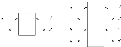
Informally, abipartite systemconsists of two subsystem, which we refer to as the left and the right subsystem. Upon inputato the left and input a0 to the right subsystem, the left subsystem outputsxand the right subsystem outputsx0(see Figure 1, left). Formally, the behavior of such a system is given by a conditional distribution q(x, x0|a, a0), with the interpretation that given input (a, a0), the system outputs a specific pair (x, x0) with probability q(x, x0|a, a0). Note that we leave the sets A,A0,X and X0, from which a, a0, x and x0 are respectively
sampled, implicit.
If we do not put any restriction upon the system, thenany conditional dis-tribution q(x, x0|a, a0) is eligible, i.e., describes a bipartite system. However, we
compute deterministic functions, we give the two subsystemshared randomness, thenq(x, x0|a, a0) may be of the form
q(x, x0|a, a0) =X r
p(r)·δ(x|a, r)·δ(x0|a0, r)
for a distributionp(r) and conditional Dirac distributionsδ(x|a, r) andδ(x0|a0, r).
Such a system is called classical or local. Interestingly, this is not the end of the story. By the laws of quantum mechanics, if the two subsystems share an entangled quantum state and obtain x and x0 without communication as the result of local measurements that may depend on a and a0, respectively, then this gives rise to conditional distributionsq(x, x0|a, a0) of the form
q(x, x0|a, a0) =ψ E
a x⊗F
a0
x0
ψ
,
where |ψi is a quantum state and {Exa}x and {Fa
0
x0}x0 are so-called POVMs.
What this exactly means is not important for us; what is important is that this leads to astrictly largerclass of bipartite systems. This is typically referred to as a violation of Bell inequalities [1], and is nicely captured by the notion of nonlocal games. A famous example is the so-called CHSH-game [3], which is closely connected to the example two-prover commitment scheme from the introduction, and which shows that the variant considered in [4] is insecure against quantum attacks.
The largest possible class of bipartite systems that is compatible with the requirement that the two subsystem do not communicate, but otherwise does not assume anything on the available resources and/or the underlying physical theory, are the so-callednon-signalingsystems, defined as follows.
Definition 2. A conditional distribution q(x, x0|a, a0) is called a non-signaling (one-round) bipartite system if it satisfies
q(x|a, a0) =q(x|a) (NS)
as well as with the roles of the primed and unprimed variables exchanged, i.e.,
q(x0|a, a0) =q(x0|a0) (NS0)
Recall that, by the convention in Remark 1, the equality (NS) is to be understood in the sense thatq(x|a, a0) does not depend ona0, i.e., thatq(x|a, a01) =q(x|a, a02) for alla01, a02, and correspondingly for (NS0).
We emphasize that this is theminimal necessary condition for the require-ment that the two subsystems do not communicate. Indeed, if e.g. q(x|a, a01)6=
The non-signaling requirement for a bipartite system is — conceptually and formally — equivalent to requiring that the two subsystems can (in principle) be queriedin any order. Conceptually, it holds because the left subsystem should be able to deliver its outputs beforethe right subsystem has received any input if and only if the output does not depend on the right subsystem’s input (which means that no information is communicated from right to left), and similarly the other way round. And, formally, we see that the non-signaling requirement from Definition 2 is equivalent to asking thatq(x, x0|a, a0) can be written as
q(x, x0|a, a0) =q(x|a)·q(x0|x, a, a0) and q(x, x0|a, a0) =q(x0|a0)·q(x|x0, a, a0)
for some respective conditional distributions q(x|a) and q(x0|a0). This charac-terization is a convenient way to “test” whether a given bipartite system is non-signaling without doing the maths.
Clearly, all classical systems are non-signaling. Also, any quantum system is non-signaling.3But there are non-signaling systems that are not quantum (and thus in particular not classical). The typical example is the NL-box (non-local box; also known asPR-box) [11], which, upon input bitsaanda0outputsrandom
output bitsxandx0 subject to
x⊕x0 =a·a0.
This system is indeed non-signaling, as it can be queried in any order: submit
ato the left subsystem to obtain a uniformly randomx, and then submita0 to the right subsystem to obtainx0:=x⊕a·b, and correspondingly the other way round.
3.2 Two-Round Systems
We now consider bipartite systems as discussed above, but where one can interact with the two subsystems multiple times. We restrict to two rounds: after having inputato the left subsystem and obtainedxas output, one can now inputbinto the left subsystem and obtain outputy, and similarly with the right subsystem (see Figure 1, right). In such a two-round setting, the non-signaling condition needs to be paired with causality, which captures that the output of the first round does not depend on the input that will be given in the second round.
Definition 3. A conditional distributionq(x, x0, y, y0|a, a0, b, b0)is called a non-signaling two-round bipartite system if it satisfies the following two causality constraints
q(x, x0|a, a0, b, b0) =q(x, x0|a, a0) (C1)
and q(x0|x, y, a, a0, b, b0) =q(x0|x, y, a, a0, b) (C2)
3 Indeed, the two parts of an entangled quantum state can be measured in any order,
a0
x0 a
x
b b0
y y0
a0
x0 a
x
Fig. 1.A one-round (left) and two-round (right) bipartite system.
and the following two non-signaling constraints
q(x, y|a, a0, b, b0) =q(x, y|a, b) (NS1)
and q(y|x, x0, a, a0, b, b0) =q(y|x, x0, a, a0, b) (NS2)
as well as with the roles of the primed and unprimed variables exchanged.
(C1) captures causality of the overall system, i.e., when considering the left and the right system as one “big” multi-round system. (C2) captures that no matter what interaction there is with the left system, the right system still satisfies causality. Similarly, (NS1) captures that the left and the right system are non-signaling over both rounds, and (NS2) captures that no matter what interaction there was in the first round, the left and the right system remain non-signaling in the second round.
It is rather clear that these arenecessaryconditions; we argue that they are sufficientto capture a non-signaling two-round system in the full version [6].
3.3 Two-Prover Commitments
We consider two-prover commitments of the following form. To commit to bit
b, the two provers P and Q receive respective “questions” a and a0 from the verifierV, and they compute, without communicating with each other, respective repliesxandx0 and send them toV. To open the commitment,P and Qsend respectivelyyandy0. Finally,V performs some check to decide whether to accept or not.
In case of classical provers P and Q, restricting the opening phase to one round with one-way communication is without loss of generality: one may always assume that in the opening phasePandQsimply reveal the shared randomness, and V checks whether x and x0 had been correctly computed, consistent with
the claimed bitb. Restricting the commit phase to one round is, as far as we can see,notwithout loss of generality; we discuss the multi-round case later.
Formally, this can be captured as follows.
andp1(x, x0, y, y0|a, a0), and an acceptance predicateAcc(x, x0, y, y0|a, a0, b). We say that Com is classical/quantum/non-signaling if p0(x, x0, y, y0|a, a0) and
p1(x, x0, y, y0|a, a0) are both classical/quantum/non-signaling when parsed as bi-partite one-round systemspb((x, y),(x0, y0)|a, a0). By default, any two-prover com-mitment scheme Comis assumed to be non-signaling.
The distribution p(a, a0) captures how V samples the “questions” a and a0,
pb(x, x0, y, y0|a, a0) describes the choices ofxandx0and ofyandy0, given that the bit to commit to isb, and Acc(x, x0, y, y0|a, a0, b) determines whetherV accepts the opening or not. Whether a scheme is classical, quantum or non-signaling captures the restrictions of the honest provers.
Given a two-prover commitment schemeCom, we define
Prob[Acc|b] := X a,a0,x,x0,y,y0
p(a, a0)·pb(x, x0, y, y0|a, a0)·Acc(x, x0, y, y0|a, a0, b),
which is the probability that a correctly formed commitment to bitbis success-fully opened.
Definition 5. A commitment scheme Com is θ-sound if Probp[Acc|b] ≥ θ for
b∈ {0,1}. We say that it isperfectly soundif it is 1-sound.
It will be convenient to write p(x0, x00, y0, y00|a, a0) instead of p0(x, x0, y, y0|a, a0) and p(x1, x01, y1, y01|a, a0) instead of p1(x, x0, y, y0|a, a0). Switching to this nota-tion, the hiding property is expressed as follows.
Definition 6. Com is called ε-hidingif d p(x0, x00|a, a0), p(x1, x01|a, a0)
≤ε for all a, a0. If Comis0-hiding, we also say it isperfectly hiding.
Capturing the binding property is more subtle. From the classical approach of defining the binding property for a commitment scheme, one is tempted to require that once the commit phase is over and a, a0, x and x0 are fixed,
ad-versarial provers ˆP and ˆQ cannot come up with an opening to b = 0 and si-multaneously with an opening to b = 1, i.e., with y0, y00 and y1, y01 such that
Acc(x, x0, y0, y00|a, a0, b = 0) and Acc(x, x0, y1, y10|a, a0, b= 1) are both satisfied (except with small probability). However, as pointed out by Dumais, Mayers and Salvail [5], in the context of a general physical theory wherey andy0 may possibly be obtained as respective outcomes of destructivemeasurements (as is the case in quantum mechanics), such a definition is too weak. It does not ex-clude that ˆP and ˆQ can freely choose to open the commitment tob = 0 or to
b= 1, whatever they want, but they cannot do both simultaneously; once they have produced one opening, their respective states got disturbed and the other opening can then not be obtained anymore.
Our definition for the binding property is based on the following game be-tween the (honest) verifierV and the adversarial provers ˆP, ˆQ.
2. V sends a bitb∈ {0,1}to ˆP and ˆQ.
3. ˆP and ˆQtry to open the commitment tob: they prepareyand y0 and send
them toV.
4. V checks if the verification predicateAcc(x, x0, y, y0|a, a0, b) is satisfied.
We emphasize that even though in the actual binding game above,the same bit b is given to the two provers, we require that the response of the provers is well determined by their strategy even in the case that b 6=b0. Of course, if the provers are allowed to communicate, they are able to detect when b 6= b0
and could reply with, e.g., y = y0 = ⊥ in that case. However, if we restrict to non-signaling provers, we assume that it isphysicallyimpossible for them to communicate with each other and distinguish the case ofb=b0 fromb6=b0.
As such, a non-signaling attack strategy against the binding property of a two-prover commitment scheme Com is given by a non-signaling two-round bipartite systemq(x, x0, y, y0|a, a0, b, b0), as specified in Definition 3. For any such bipartite system, representing a strategy for ˆP and ˆQ in the above game, the probability that ˆP and ˆQwin the game, in thatAcc(x, x0, y, y0|a, a0, b) is satisfied
when they have to open to the bitb, is given by
Prob∗q[Acc|b] := X a,a0,x,x0,y,y0
p(a, a0)·q(x, x0, y, y0|a, a0, b, b)·Acc(x, x0, y, y0|a, a0, b).
We are now ready to define the binding property.
Definition 7. A two-prover commitment scheme Com is δ-binding (against non-signaling attacks) if it holds for any non-signaling two-round bipartite sys-tem q(x, x0, y, y0|a, a0, b, b0)that
Prob∗q[Acc|0] + Prob∗q[Acc|1]≤1 +δ .
In other words, a scheme isδ-binding if in the above game the dishonest provers win with probability at most (1 +δ)/2 when b ∈ {0,1} is chosen uniformly at random. If a commitment scheme is binding (for a small δ) in the sense of Definition 7, then for any strategyqfor ˆP and ˆQ, they can just as wellhonestly commit to a bit ˆb, where ˆbis set to 0 with probabilityp0= Prob∗q[Acc|0] and to 1 with probabilityp1= 1−p0≈Prob∗q[Acc|1], and they will have essentially the same respective success probabilities in opening the commitment tob = 0 and tob= 1.
4
Impossibility of Two-Prover Commitments
4.1 Simple Schemes
We first consider a special, yet natural, class of schemes. We call a two-prover commitment schemeComsimpleif it has the same communication pattern as the scheme described in the introduction. More formally, it is called simple ifa0, x0
andyare “empty” (or fixed), i.e., ifComis given byp(a),p0(x, y0|a),p1(x, y0|a) and Acc(x, y0|a, b); to simplify notation, we then write y instead ofy0. In other words, P is only involved in the commit phase, where, in order to commit to bit b, he outputsxupon inputa, andQis only involved in the opening phase, where he outputs y. The non-signaling requirement forCom then simplifies to
pb(y|a) =pb(y). Recall that by our convention, we may writep(x0, y0|a) instead ofp0(x, y|a) andp(x1, y1|a) instead of p1(x, y|a).
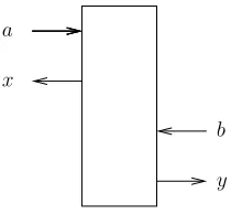
In case of such a simple two-prover commitment schemeCom, a non-signaling two-prover strategy reduces to a non-signaling one-round bipartite system as specified in Definition 2 (see Figure 2).
a
x
b
y
Fig. 2.The adversaries’ strategyq(x, y|a, b) in case of asimplecommitment scheme.
As a warm-up exercise, we first consider a simple two-prover commitment scheme that isperfectly hidingandperfectly sound. Recall that formally, a simple scheme is given by p(a),p0(x, y|b), p1(x, y|a) andAcc(x, y|a, b), and the perfect hiding property means that p0(x|a) = p1(x|a) for any a. To show that such a scheme cannot be binding, we have to show that there exists a non-signaling one-round bipartite system q(x, y|a, b) such that Prob∗q[Acc|0] + Prob∗q[Acc|1] is significantly larger than 1. But this is actually trivial: we can simply set
q(x, y|a, b) :=pb(x, y|a). It then holds trivially that
Prob∗q[Acc|b] = X a,x,y
p(a)q(x, y|a, b)Acc(x, y|a, b)
= X
a,x,y
p(a)pb(x, y|a)Acc(x, y|a, b)
= Probp[Acc|b]
to be verified is thatq(x, y|a, b) is non-signaling, i.e., thatq(x|a, b) =q(x|a) and
q(y|a, b) =q(y|b). To see that the latter holds, note thatq(y|a, b) =pb(y|a), and becauseComis non-signaling we have thatpb(y|a) =pb(y), i.e., does not depend on a. Thus, the same holds for q(y|a, b) and we have q(y|a, b) = q(y|b). The former condition follows from the (perfect) hiding property:q(x|a, b) =pb(x|a) =
pb0(x|a) =q(x|a, b0) for arbitraryb, b0 ∈ {0,1}, and thus q(x|a, b) =q(x|a).
Below, we show how to extend this result to non-perfectly-binding simple schemes. In this case, we cannot simply set q(x, y|a, b) := pb(x, y|a), because such a q would not be non-signaling anymore — it would merely be “almost non-signaling”. Instead, we have to find a strategyq(x, y|a, b) that is (perfectly) non-signaling and close to pb(x, y|a); we will find such a strategy with the help of Lemma 1. In Section 4.2, we will then consider general schemes where both provers interact with the verifier in both phases. In this general case, further complications arise.
Theorem 1. Consider a simple two-prover commitment scheme Com that is
ε-hiding. Then, there exists a non-signaling strategyq(x, y|a, b)such that
Prob∗q[Acc|0] = Probp[Acc|0] and Prob∗q[Acc|1]≥Probp[Acc|1]−ε .
If Comis perfectly sound, it follows that
Prob∗q[Acc|0] + Prob∗q[Acc|1]≥1 + (1−ε)
and thus it cannot be δ-binding forδ <1−ε.
Proof. Recall that Com is given by p(a), pb(x, y|a) and Acc(x, y|a, b), and we write p(xb, yb|a) instead of pb(x, y|a). Because Com is ε-hiding, it holds that
d p(x0|a), p(x1|a)
≤ ε for any fixed a. Thus, using Lemma 1 for every a, we can glue together p(x0, y0|a) and p(x1, y1|a) along x0 and x1 to obtain a distribution p(x0, x1, y0, y1|a) such that p(x0 6= x1|a) ≤ ε, and in particular
d p(x0, y1|a), p(x1, y1|a)
≤ε.
We define a strategy q for the dishonest provers by setting q(x, y|a, b) :=
p(x0, yb|a) (see Figure 3). First, we show that q is non-signaling. Indeed, we have q(x|a, b) =p(x0|a) for anyb, soq(x|a, b) =q(x|a), and we haveq(y|a, b) =
p(yb|a) =p(yb) for anya, and thusq(y|a, b) =q(y|b).
As for the acceptance probability, forb= 0 we haveq(x, y|a,0) =p(x0, y0|a) and as such Prob∗q[Acc|0] equals Probp[Acc|0]. Forb= 1, we have
d q(x, y|a,1), p(x1, y1|a)
=d p(x0, y1|a), p(x1, y1|a)
≤ε
and since the statistical distance does not increase under data processing, it follows that Probp[Acc|1] and Prob∗q[Acc|1] areε-close; this proves the claim. ut
The bound on the binding property in Theorem 1 is tight, as the following theorem shows. The proof is given in the full version [6].
a
x1 y1
a
x0
b
yb
a
x0 y0
Fig. 3.Defining the strategyqby gluing togetherp(x0, y0|a) andp(x1, y1|a).
4.2 Arbitrary Schemes
We now remove the restriction on the scheme to be simple. As before, we first consider the case of a perfectly hiding scheme.
Theorem 3. Let Com be a single-round two-prover commitment scheme. If
Com is perfectly hiding, then there exists a non-signaling two-prover strategy
q(x, x0, y, y0|a, a0, b, b0) such that
Prob∗q[Acc|b] = Probp[Acc|b]
forb∈ {0,1}.
Proof. Combeing perfectly hiding means thatd(p(x0, x00|a, a0), p(x1, x01|a, a0)) = 0 for all a and a0. Gluing together the distributions p(x0, x00, y0, y00|a, a0) and
p(x1, x01, y1, y10|a, a0) along (x0, x00) and (x1, x01) for every (a, a0), we obtain a distribution p(x0, x00, x1, x01, y0, y00, y1, y01|a, a0) with the correct marginals and
p((x0, x00) 6= (x1, x01)|a, a0) = 0. That is, we have x0 = x1 and x00 = x01 with certainty. We now define a strategy for dishonest provers as (Figure 4)
q(x, x0, y, y0|a, a0, b, b0) :=p(x0, x00, yb, y0b0|a, a0).
Since p(x0, x00, yb, yb0|a, a0) = p(xb, x0b, yb, y0b|a, a0), it holds that Prob
∗
q[Acc|b] = Probp[Acc|b]. It remains to show that this distribution satisfies the non-signaling and causality constraints (C1) up to (NS2) of Definition 3. This is done below.
– For (C1), note that summing up over y and y0 yields q(x, x0|a, a0, b, b0) =
p(x0, x00|a, a0), which indeed does not depend onbandb0.
– For (NS1), note that q(x, y|a, a0, b, b0) = p(x0, yb|a, a0) = p(xb, yb|a, a0) =
p(xb, yb|a), where the last equality holds by the non-signaling property of
p(xb, yb|a, a0).
– For (C2), first note that
q(x, x0, y|a, a0, b, b0) =p(x0, x00, yb|a, a0) (2)
which does not depend onb0. We then see that (C2) holds by dividing by
q(x, y|a, a0, b, b0) =p(x
0, yb|a, a0).
a
x0
b
yb yb00
b0 x0
0
a0 a
x1
y1
a0
x0
1
y0
1
a
x0
y0
a0
x0
0
y0
0
Fig. 4.Definingqfromp(x0, x00, y0, y00|a, a0) andp(x1, x01, y1, y01|a, a0) glued together.
The properties (C1) to (NS2) with the roles of the primed and unprimed variables exchanged follows from symmetry. This concludes the proof. ut
The case of non-perfectly hiding schemes is more involved. At first glance, one might expect that by proceeding analogously to the proof of Theorem 3 — i.e., gluing togetherp(x0, x00, y0, y00|a, a0) andp(x1, x01, y1, y10|a, a0) along (x0, x00) and (x1, x01) and definingqthe same way — one can obtain a strategyqthat succeeds with probability 1−εif the scheme isε-hiding. Unfortunately, this approach fails because in order to show (NS1) we use thatp(x0, y1|a, a0) =p(x1, y1|a, a0) which in general does not hold for commitment schemes that are not perfectly hiding. As a consequence, our proof is more involved, and we have a constant-factor loss in the parameter.
Theorem 4. Let Com be a single-round two-prover commitment scheme and suppose that it isε-hiding. Then there exists a non-signaling two-prover strategy
q(x, x0, y, y0|a, a0, b, b0) such that
Prob∗q[Acc|0] = Probp[Acc|0] and Probq∗[Acc|1]≥Probp[Acc|1]−5ε .
Thus, ifComis perfectly sound, it is at best(1−5ε)-binding.
To prove this result, we use two lemmas. In the first one, we add the additional assumptions thatp(x0|a, a0) =p(x1|a, a0) andp(x00|a, a0) =p(x01|a, a0). The sec-ond one shows that we can tweak an arbitrary scheme in such a way that these additional conditions hold. The proofs are given in the full version [6].
Lemma 2. Let Combe aε-hiding two-prover commitment scheme with the ad-ditional property thatp(x0|a, a0) =p(x1|a, a0)andp(x00|a, a0) =p(x01|a, a0). Then, there exists a non-signaling p0(x1, x01, y1, y10|a, a0) such that
d p0(x1, x01, y1, y10|a, a
0), p(x
1, x01, y1, y10|a, a
0)
≤ε
andp0(x1, x01|a, a0) =p(x0, x00|a, a0).
Lemma 3. LetCombe aε-hiding two-prover commitment scheme. Then, there exists a non-signalingp˜(x1, x01, y1, y01|a, a0)such that
d p˜(x1, x10, y1, y01|a, a0), p(x1, x01, y1, y01|a, a0)
≤2ε
which has the property thatp˜(x1|a, a0) =p(x0|a, a0)andp˜(x01|a, a0) =p(x00|a, a0).
With these two lemmas, Theorem 4 is easy to prove.
Proof (Theorem 4). We start with a ε-hiding non-signaling bit-commitment schemeCom. We apply Lemma 3 and obtain ˜p(x1, x01, y1, y01|a, a0) that is 2ε-close to p(x1, x01, y1, y10|a, a0) and satisfies ˜p(x1|a, a0) = p(x0|a, a0) and ˜p(x01|a, a0) =
p(x00|a, a0). Furthermore, by triangle inequality
d p˜(x1, x01|a, a
0), p(x
0, x00|a, a
0)
≤3ε .
Thus, replacingp(x1, x01, y1, y1|a, a0) by ˜p(x1, x01, y1, y01|a, a0) gives us a 3ε-hiding two-prover commitment scheme that satisfies the extra assumption in Lemma 2. As a result, we obtain a distribution p0(x1, x01, y1, y01|a, a0) that is 3ε-close to ˜
p(x1, x01, y1, y10|a, a0), and thus 5ε-close top(x1, x01, y1, y10|a, a0), with the property thatp0(x1, x01|a, a0) =p(x0, x00|a, a0). Therefore, replacing ˜p(x1, x10, y1, y10|a, a0) by
p0(x1, x01, y1, y10|a, a0) gives us aperfectly-hidingtwo-prover commitment scheme, to which we can apply Theorem 3. As a consequence, there exists a non-signaling strategyq(x, x0, y, y0|a, a0) with Prob∗q[Acc|0] = Probp[Acc|0] and Prob
∗
q[Acc|1]≥ Probp[Acc|1]−5ε, as claimed.
Remark 5. If Com already satisfies p(x0|a, a0) = p(x1|a, a0) and p(x00|a, a0) =
p(x01|a, a0), we can apply Lemma 2 right away and thus get a strategyq with Prob∗q[Acc|0] = Probp[Acc|0] and Prob∗q[Acc|1] ≥Probp[Acc|1]−ε. Thus, with this additional condition, we still obtain a tight bound as in Theorem 1.
4.3 Multi-Round Schemes
We briefly discuss a limited extension of our impossibility results for single-round schemes to schemes where during the commit phase, there is multi-round inter-action between the verifierV and the two proversP andQ. We still assume the opening phase to be one-round; this is without loss of generality in case of clas-sical two-prover commitment schemes (where the honest provers are restricted to be classical). In this setting, we have the following impossibility result, which is restricted to perfectly-hiding schemes.
Theorem 5. LetCombe a multi-round two-prover commitment scheme. IfCom
is perfectly hiding, then there exists a non-signaling two-prover strategy that com-pletely breaks the binding property, in the sense of Theorem 3.
this definition, the proof is a straightforward extension of the proof of Theorem 3: the non-signaling strategy is obtained by gluing together p(x0,x00|a,a0) and
p(x1,x01|a,a0) along (x0,x00) and (x1,x01), and setting q(x,x0, y, y0|a,a0, b, b0) :=
p(x0,x00, yb, y0b0|a,a0), where we use bold-face notation for the vectors that
col-lect the messages sent during the multi-round commit phase: a collects all the messages sent by the verifier to the proverP, etc.
As far as we see, the proof of the non-perfect case, i.e. Theorem 4, does not generalize immediately to the multi-round case. As such, proving the impossibil-ity ofnon-perfectly-hiding multi-roundtwo-prover commitment schemes remains an open problem.
5
Possibility of Three-Prover Commitments
It turns out that we can overcome the impossibility results by adding a third prover. We will describe a scheme that is perfectly sound, perfectly hiding and 2−n-binding with communication complexityO(n). We now define what it means for three provers to be non-signaling; since our scheme is similar to a simple scheme, we can simplify this somewhat. We consider distributionsq(x, y, z|a, b, c) whereaandxare input and output of the first proverP,bandy are input and output of the second prover Q and c and z are input and output of the third proverR.
Definition 8. A conditional distributionq(x, y, z|a, b, c)is called anon-signaling (one-round) tripartite systemif it satisfies
q(x|a, b, c) =q(x|a), q(y|a, b, c) =q(y|b), q(z|a, b, c) =q(z|c),
and
q(x, y|a, b, c) =q(x, y|a, b),q(x, z|a, b, c) =q(x, z|a, c),q(y, z|a, b, c) =q(y, z|b, c).
In other words, for any way of viewingqas a bipartite system by dividing in- and outputs consistently into two groups, we get a non-signaling bipartite system.
We restrict to simple schemes, where during the commit phase, only P is active, sending x upon receiving a from the verifier, and during the opening phase, onlyQand Rare active, sendingy andz to the verifier, respectively.
Definition 9. A simple three-prover commitment scheme Com consists of a probability distributionp(a), two distributionsp0(x, y, z|a)andp1(x, y, z|a), and an acceptance predicate Acc(x, y, z|a, b).
It is called classical/quantum/non-signaling if pb(x, y, z|a) is, when understood as a tripartite system pb(x, y, z|a,∅,∅) with two “empty” inputs.
Soundness and the hiding-property are defined in the obvious way. As for the binding property, for a simple three-prover commitment schemeComand a non-signaling strategyq(x, y, z|a, b, c), let
Prob∗q[Acc|b] = X a,x,y,z
We say thatComisδ-binding if
Prob∗q[Acc|0] + Probq∗[Acc|1]≤1 +δ.
Theorem 6. For every positive integer n, there exists a classical simple three-prover commitment scheme that is perfectly sound, perfectly hiding and 2−n -binding. The verifier communicates nbits to the first prover and receives nbits from each prover.
The scheme that achieves this is essentially the same as the example two-prover scheme described in the introduction, except that we add a third prover that imitates the actions of the second. To be more precise: the provers P, Q and
R have as shared randomness a uniformly randomr ∈ {0,1}n. The verifier V chooses a uniformly random a∈ {0,1}n and sends it toP. As commitment,P returnsx:=r⊕a·b. To open the commitment tob,Qand Rsend y:=r and
z:=rtoV who accepts if and only ify=z andx=y⊕a·b.
Before beginning with the formal proof that this scheme has the properties stated in our theorem, we give some intuition. Let a and x be the input and output of the dishonest first prover, P. To succeed, the second prover Q has to produce outputx⊕a·b where b is the second prover’s input and the third proverRhas to producex⊕a·cwherecis the third prover’s input. Our theorem implies that a strategy which always produces these outputs must be signaling. Why is that the case?
In the game that defines the binding-property, we always haveb=c, but the dishonest provers must obey the non-signaling constraint even in the “impossi-ble” case thatb6=c. Let us consider the XOR ofQ’s output and R’s output in the case that b 6=c: we get (x⊕a·b)⊕(x⊕a·c) =a·b⊕a·c = a. But in the non-signaling setting, the joint distribution of Q’s andR’s output may not depend ona. Thus, the strategy we suggested does not satisfy the non-signaling constraint. Let us now prove the theorem.
Proof (Theorem 6).It is easy to see that the scheme is sound. Furthermore, for every fixed aand b,pb(x|a) is uniform, so the scheme is perfectly hiding. Now consider a non-signaling strategyqfor dishonest provers. The provers succeed if and only if y=z=x⊕a·b. Define q(a, x, y, z|b, c) =p(a)·q(x, y, z|a, b, c). The non-signaling property implies that
q(y=x⊕a·b|a, b, c= 0) =q(y=x⊕a·b|a, b, c= 1) and (3)
q(z=x⊕a·c|a, b= 0, c) =q(z=x⊕a·c|a, b= 1, c). (4)
It follows that
Prob∗q[Acc|0] + Prob∗q[Acc|1]
=q(y=x⊕a·b, z=x⊕a·c|b= 0, c= 0)
+q(y=x⊕a·b, z=x⊕a·c|b= 1, c= 1)
=q(y=x⊕a·b|b= 0, c= 1) +q(z=x⊕a·c|b= 0, c= 1)
by Equations (3) and (4)
≤1 +q(y=x⊕a·b, z=x⊕a·c|b= 0, c= 1) by Equation (1)
It now remains to upper-boundq(y=x⊕a·b, z=x⊕a·c|b= 0, c= 1). Since
p(a) is uniform andq(y, z|a, b, c) is independent ofa, we have
q(y=x⊕a·b, z=x⊕a·c|b= 0, c= 1)≤q(y⊕z=a|b= 0, c= 1) = 1 2n
and thus our scheme is 2−n-binding. ut
Remark 6. The three-prover scheme above has the drawback that two provers are involved in the opening phase; as such, there needs to be agreement on whether to open the commitment or not; if there is disagreement then this may be problematic in certain applications. However, P and Q are not allowed to communicate. One possible solution is to haveV forward anauthenticated“open” or “not open” message fromP toQandR. This allows for some communication from P to Q and R, but if the size of the authentication tag is small enough compared to the security parameter of the scheme, i.e., n, then security is still ensured.
Acknowledgements We would like to thank Claude Cr´epeau for pointing out the issue addressed in Remark 6 and the solution sketched there, and Jed Kaniewski for helpful discussions regarding relativistic commitments.
References
1. John Stewart Bell. On the Einstein-Podolsky-Rosen paradox. Physics, 1:195–200, 1964.
2. Michael Ben-Or, Shafi Goldwasser, Joe Kilian, and Avi Wigderson. Multi-Prover Interactive Proofs: How to Remove Intractability Assumptions. In Janos Simon, editor,STOC, pages 113–131. ACM, 1988.
3. John F. Clauser, Michael A. Horne, Abner Shimony, and Richard A. Holt. Proposed experiment to test local hidden-variable theories.Phys. Rev. Lett., 23:880–884, Oct 1969.
4. Claude Cr´epeau, Louis Salvail, Jean-Raymond Simard, and Alain Tapp. Two Provers in Isolation. In Dong Hoon Lee and Xiaoyun Wang, editors,ASIACRYPT, volume 7073 ofLecture Notes in Computer Science, pages 407–430. Springer, 2011. 5. Paul Dumais, Dominic Mayers, and Louis Salvail. Perfectly concealing quantum bit commitment from any quantum one-way permutation. In Bart Preneel, editor, EUROCRYPT, volume 1807 ofLecture Notes in Computer Science, pages 300–315. Springer, 2000.
6. Serge Fehr and Max Fillinger. Multi-Prover Commitments Against Non-Signaling Attacks. ArXiv e-prints, 2015. http://arxiv.org/abs/1505.03040.
8. Adrian Kent. Unconditionally secure bit commitment. Phys. Rev. Lett., 83:1447– 1450, 1999.
9. Hoi-Kwong Lo and H. F. Chau. Is quantum bit commitment really possible?Phys. Rev. Lett., 78:3410–3413, Apr 1997.
10. Dominic Mayers. Unconditionally Secure Quantum Bit Commitment is Impossible. Phys. Rev. Lett., 18:3414–3417, 1997.
11. Sandu Popescu and Daniel Rohrlich. Quantum nonlocality as an axiom. Founda-tions of Physics, 24(3):379–385, 1994.
12. Peter Rastall. Locality, bell’s theorem, and quantum mechanics. Foundations of Physics, 15(9):963–972, 1985.
13. Renato Renner and Robert K¨onig. Universally Composable Privacy Amplification Against Quantum Adversaries. In Joe Kilian, editor,TCC, volume 3378 ofLecture Notes in Computer Science, pages 407–425. Springer, 2005.
14. Boris S. Tsirelson and Leonid A. Khalfin. Quantum and quasi-classical analogs of Bell inequalities. In Symposium on the Foundations of Modern Physics, pages 441–460, 1985.