STABILITY CONSTRAINTS USING THE
EVOLUTIONARY OPTIMISATION METHOD
by
Dhayanthi Manickarajah, BSc, MEiigSc
A thesis submitted in fulfilment of the requirements for the Degree of
DOCTOR OF PHILOSOPHY
Faculty Engineering and Science
Victoria University of Technology
Melbourne, Victoria 8001, Australia
This thesis does not contain any material, which has been previously submitted for a degree or diploma at any university. Except where due reference is made in the text, the work described in this thesis is the result of the candidate's own investigations.
PM
/•V--U,x-XCandidate
ACKNOWLEDGEMENTS
I sincerely thank Professor Mike Xie for the supervision that he provided throughout this dissertation. His advice on technical matters, constant encouragement and motivation, ready accessibility and constructive criticism are greatly acknowledged. He made every effort to ensure that I was provided with excellent equipment and a comfortable working environment. In addition, Mike encouraged me to attend conferences and to publish our findings in international journals and sought all possible avenues to further my knowledge. Also Mike's keen interest in the topic, Evolutionary Structural Optimisation gave me inspiration to accomplish in the area of research covered.
I am also grateful to the Faculty of Engineering, Victoria University of Technology and in particular to the former Dean of Faculty of Engineering, Professor Ian Johnson for the Dean's Research Scholarship that I received, providing financial support throughout this study.
I wish to thank Professor Grant Steven from the Department of Aeronautical Engineering, University of Sydney for allowing me to get access to some source codes of STRAND6 finite element analysis software, which enabled me to carry out the research.
Study. I would also like to express my appreciation to the technical staff of the Department in particular to Mr. Jack Li for their help.
I thank my fellow postgraduates, Aftab, Annie, Gali, Gavin, Mahesh, Nelum, Nha, Nina, Rahman, Sujay and Sunil, for the invaluable friendship and support provided during my stay at Victoria University. I wish you all the very best in the future and hope that we will always be friends.
SUMMARY
In the past most of the works on structural optimisation have been based on either mathematical programming or optimality criteria methods and have mainly concentrated on static responses of structures. These optimisation methods are mathematically complex and have limited applications. A novel approach to structural optimisation is being developed for practical applications based on the concept of slowly removing the inefficient material or gradually shifting the material from the strongest part of the structure to the weakest part until the structure evolves towards the desired optimum. From the results of finite element analysis, the contribution of each element to the required structural response may be assessed. Based on this assessment, material is gradually shifted or removed in the design domain. In doing so optimum designs can be easily achieved without resorting to any complex mathematics. This optimisation procedure is called Evolutionary Structural Optimisation (ESO). Compared to other methods for structural optimisation, ESO is overwhelmingly attractive due to its simplicity and effectiveness. ESO has been demonstrated to be capable of solving many problems of size, shape and topology optimisation.
This project examines the suitability of the ESO for the design of structures with buckling constraints. In recent years, more attention has been focused on stability and dynamic responses of structures. With the use of high strength materials and robust design methods, many structural elements are becoming thinner and more slender which makes them more susceptible to buckling. Structural optimisation for problems with buckling constraints is complicated because the calculation of buckling loads requires the solution of the prebuckling stress distribution (static analysis) and then the eigenvalue solution (buckling analysis) at each optimisation step.
TABLE OF CONTENTS Page No.
DECLARATION ii
ACKNOWLEDGEMENTS iii
SUMMARY V
TABLE OF CONTENTS vi
PRINCIPAL NOTATIONS AND ABBREVIATIONS xii
CHAPTER 1 - INTRODUCTION
1.1 General 1-1 1.2 Structural Optimisation 1 -3
1.2.1 Classifications 1 -6
1.2.2 Major approaches 1-7
1.3 Aims of the Project 1-11 1.4 Significance of the Project 1-12
1.5 Layoutof the Thesis 1-14
CHAPTER 2 - LITERATURE REVIEW
2.1 Introduction 2-1 2.2 Optimum Design of Columns 2-1
2.3 Optimum Design of Frames 2-4 2.4 Optimum Design of Plates 2-10
CHAPTER 3 - EVOLUTIONARY STRUCTURAL OPTIMISATION (ESO)
3.1 Introduction 3-1 3.2 Basic Concept and General Steps in ESO 3-2
3.2.1 ESO for structures with stress criterion 3-3 3.2.2 ESO for structures with displacements and stiffness constraints 3-7
3.2.3 ESO for problems with frequency constraints 3-12 3.3 Implementation of ESO Methods into Finite Element Codes 3-15
3.4 Discussion on Existing ESO Methods 3-16
3.5 Summary 3-19
CHAPTER 4 - ESO FOR STRUCTURES AGAINST BUCKLING
4.1 Introduction 4-1 4.2 Buckling Analysis of Structures 4-2
4.3 Sensitivity Number for Buckling Load - Simple Eigenvalue 4-4
4.3.1 Sensitivity number for element removal 4-5 4.3.2 Sensitivity number for element resizing 4-6 4.4 Evolutionary Procedure for Buckling Optimisation 4-8
4.5 Examples 4-13 4.5.1 Examples of column optimisation 4-13
4.5.2 Examples of frame optimisation 4-16 4.5.2.1 Optimum design of a three member portal frame 4-16
4.7 Optimality Criteria Methods Based on Uniform Strain Energy Concept 4-29
4.7.1 Optimality criterion by Khot et al. (1976) 4-29 4.7.2 Optimality criterion by Szyszkowski and Watson (1988) 4-32
4.8 Conclusions 4-35
CHAPTER 5 - OPTIMUM DESIGN OF MULTIMODAL STRUCTURES
5.1 Introduction 5-1 5.2 Sensitivity Number for Buckling Load of Repeated Eigenvalues 5-4
5.3 Examples 5-6 5.3.1 Clamped-clamped column 5-6
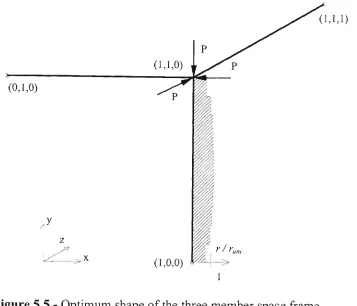
5.3.2 Three member portal frame - bimodal example 5-10 5.3.3 Three member space frame - trimodal example 5-12
5.3.4 Box frame 5-14 5.4 Multimodal Optimality Criteria by Szyszkowski (1992) 5-19
5.5 Conclusions 5-21 Appendix 5.1 5-22 Appendix 5.2 5-24
CHAPTER 6 - MINIMUM WEIGHT DESIGN OF FRAME STRUCTURES
6.1 Introduction 6-1 6.2 Uniform Scaling Factor Sb 6-2
6.2.1 Uniform scaling factor for 2-dimensional frames 6-3 6.2.2 Uniform scaling factor for space frames 6-5
6.4 Examples 6-14 6.4.1 Space frame - Example 1 6-14
6.4.2 Space frame - Example 2 6-15
6.5 Conclusions 6-17
CHAPTER 7 - OPTIMUM DESIGN OF STRUCTURES WITH MULTIPLE
LOAD CASES
7.1 Introduction 7-1 7.2 Sensitivity Number 7-2
7.3 Optimisation Procedure 7-3 7.3.1 Constant weight design 7-3
7.3.2 Minimum weight design 7-4
7.4 Examples 7-8 7.4.1 Constant weight design 7-8
7.4.2 Minimum weight design 7-12
7.5 Conclusions 7-13
CHAPTER 8 - OPTIMUM DESIGN OF STRUCTURES WITH MULTIPLE
CONSTRAINTS
8.1 Introduction 8-1 8.2 Multiple Constraints Problem 8-1
8.2.1 Sizing optimisation with stiffness constraints 8-3 8.2.2 Sizing optimisation with displacement constraints 8-4
8.2.4 Uniform scaling and critical scale factors 8-7
8.3 Sensitivity Number 8-8 8.4 Optimisation Procedure 8-9
8.5 Examples 8-11 8.5.1 50-bar truss tower 8-11
8.5.2 5-Storey frame 8-17
8.6 Conclusions 8-22
CHAPTER 9 - OPTIMUM DESIGN OF PLATE STRUCTURES
9.1 Introduction 9-1 9.2 Sensitivity Number and Optimisation Procedure 9-2
9.3 Examples 9-3 9.3.1 Simply supported square plate 9-4
9.3.2 Clamped square plate 9-8 9.3.3 Simply supported rectangular plate 9-11
9.4 Previously Reported Optimum Shapes 9-13 9.4.1 Optimum shapes by Pandey and Sherboume 9-13
9.4.2 Optimum shapes by Levy and his co-workers 9-15
9.4.3 Optimum design by Folgado et al. 9-18 9.5 Strain Energy Distribution of Optimum Plates 9-22 9.6 Buckling Analysis of Variable-thickness Plates 9-24 9.7 Eliminationof Checkerboard Patterns from 4-Node Element Designs 9-30
9.7.2 Element sensitivity number re-distribution method 9-33
9.8 Layout Optimisation 9-35
9.9 Conclusions 9-42
CHAPTER 10 - CONCLUSIONS AND FUTURE RESEARCH
10.1 Conclusions 10-1 10.2 Further Recommendations 10-5
PUBLICATIONS DURING THIS CANDIDATURE PI
PRINCIPAL NOTATIONS AND ABBREVIATIONS
Principal Notations
A - cross-sectional area
a - length of a rectangular plate
[5]/ - strain-displacement relation matrix
h - breadth of a rectangular cross-section or width of a rectangular plate
C - mean compliance
Call - allowable limit for the mean compliance
Cv - coefficient of variation
d - depth of the rectangular cross-section
dj -j d.o.f displacement component
dj - allowable limit for dj
{d} - nodal displacement vector
[di] - f element displacement vector associated with {d}
{dij} - i element displacement vector associated with {dj}
{dj} - displacement vector due to the virtual unit load vector {Fj}
E - Young's modulus
[E]i - element material property matrix
FS - factor of safety against buckling
{Fj} - virtual unit load vector aty d.o.f
/ - moment of inertia [i^l - global stiffness matrix
[Kg] - global geometric stiffness matrix
[AAT] - change in the global stiffness matrix
[AA^g] - change in the global geometric stiffness matrix [AA:,] - change in the z* element stiffness matrix L - member length
[M] - global mass matrix [mi] - i element mass matrix
nl - number of load cases
NSE - normalised specific strain energy
A'v - thickness distribution parameter OF - optimum factor
{P} - nodal force vector
r - radius of a circular cross-section
Sb - uniform scaling factor for buckling constraint
Sc ~ uniform scaling factor for stiffness constraint
Sd - uniform scaling factor for displacement constraint
SE - strain energy
Si - size of the /* element (surface area or member length)
SPE - specific strain energy
Ss - uniform scaling factor for stress constraint
t - plate thickness
tmax - allowable maximum plate thickness
tmin - allowable m i n i m u m plate thickness
tu - uniform plate thickness
{Uj} -j eigenvector
V - total volume of a structure
w - lateral deflection of the rectangular plate a, _ f element sensitivity number for removal a, _ /' element sensitivity number for size increment
a," _ f' element sensitivity number for size reduction
a/6, Oiib' and aib - sensitivity number for buckling constraint; removal, size increment and size reduction, respectively
a,c, a,c^ and a,c" - sensitivity number for stiffness constraint; removal, size increment and size reduction, respectively
ot/rf, a , / and a,/ - sensitivity number for displacement constraint; removal, size increment and size reduction, respectively
a,y, a,/" and af - sensitivity number for frequency constraint; removal, size increment and size reduction, respectively
a,-5, ais^ and a,^" - sensitivity number for stress constraint; removal, size increment and size reduction, respectively
ttM - nodal sensitivity number
a, - re- distributed modified sensitivity number s - eigenvalue multiplicity parameter
00/ - J natural frequency
Gi"" - maximum von Mises stress in the /* element
o- vm _ maximum von Mises stress in the whole structure
max
{a}/ - element stress matrix
P - dimensionless minimum cross-sectional area Xcr - critical buckling load factor
A^;' - critical buckling load factor of the uniform design ?ij' - critical buckling load factor of the optimum design ^y - j eigenvalue
p - density
a - normal stress v -Poisson's ratio T - shear stress
Abbreviations
ER - Evolutionary Rate
ESO - Evolutionary Structural Optimisation FEA - Finite Element Analysis
FSD - Fully Stressed Design MP - Mathematical Programming OC - Optimality Criteria
CHAPTER 1 - INTRODUCTION
1.1 General
The notion of an optimum solution of an engineering problem is intriguing and has been investigated for a long time. Earlier, engineering design was conceived as a kind of art that demanded great ingenuity and experience of the designer, and the development of the field was characterised by gradual evolution in terms of continual improvement of existing types of engineering designs. The design process generally was a sequential trial-and-error process where the designer's skills and experience were most important prerequisites for successful decisions for the trial phase. However, nowadays strong technological competition which requires reduction of design time and costs of products with high quality and functionality, and current emphasis on saving of energy, saving of material resources, consideration of environmental problems, etc., often involves creation of new products for which prior engineering experience is totally lacking. Development of such products must naturally resort to application of scientific methods. Hence, during recent decades, engineering design has changed from art and evolution to scientifically based methods of rational design and optimisation.
of Structural optimisation is rapidly growing in automotive, aeronautical, mechanical, civil, nuclear, naval and off-shore engineering. As the result of the growing pace of applications, research into structural optimisation methods is increasingly driven by real-life problems. This significant development has been strongly boosted by the advent of reliable and efficient general structural analysis methods such as the finite element method, design sensitivity analysis and rapid improvements in optimisation methods, along with the exponentially increasing speed and capacity of digital computers at low cost. The high performance of digital computers makes large scale structural optimisation possible and profitable in a large number of applications where thousands of design variables and constraints may need to be handled.
With the introduction of high speed computers, finite element analysis has become a very powerful tool in solving various complex structural engineering problems. After being able to determine the structural behaviour by means of finite element analysis, an important goal for engineers to achieve is to improve and optimise structural designs. In the past, the modification of a structure and the subsequent evaluation of the modified structure have been manually carried out. However, it is now possible to control repetitive modifications, re-analyses and re-evaluations automatically. Thus, a systematic improvement of structural systems may be achieved through computer simulation. In this context, structural optimisation based upon finite element method is becoming an advanced Computer Aided Design (CAD) tool.
problems solved by optimisation experts. There is an obvious gap between the progress of the optimisation theory and its application to practical design problems. The vast majority of published work deals with the mathematical aspects of structural optimisation. It has been suggested that one major reason for the gap between the theory and practice of structural optimisation is the excessive emphasis on mathematical aspects rather than structural aspects of optimisation. Often the latter are confined to rather trivial examples, intended only to illustrate the successful application of a particular structural optimisation method.
Currently the research activity is directed towards making structural optimisation methods available to practising engineers and scientists in an easy, reliable, inexpensive and mathematically less complex form so that the optimisation techniques can be promoted as a viable tool in the design office. It is important to understand the basic concepts behind the structural optimisation methods for proper application of these methods to practical problems. The complex interactions of interdisciplinary constraints and the large number of design variables of the finite element models can severely test the limits of existing methods in this context.
1.2 Structural Optimisation
constraints involved and the nature of the design variables. In general, the aim of a structural optimisation problem is formally given as:
• minimise (or maximise) objective functions subject to behavioural and geometrical constraints.
The following criteria can be used either as the objective function or as the behavioural constraint.
• Structural weight (volume), storage capacity • Cost (material, manufacturing, life cycle etc.)
• Global measure of the structural performance such as stiffness, buckling load, plastic collapse load, natural vibration frequency, dynamic response etc.
• Local structural responses such as stress, strain or displacement at prescribed points; maximum stress, strain or displacement in the whole structure; stress intensity factor etc.
Single criterion optimisation is associated with only one objective function whilst multi-criterion optimisation involves several objectives. The constraints may be given in the form of equality or inequality conditions. Since these objective functions and constraints are implicit functions of design variables, most structural optimisation problems are highly non-linear.
availability of member sizes, fabrication, physical practicability, aesthetics etc. Constraints of this kind are typically inequality constraints that specify lower and/or upper bounds on the design variables. Geometrical constraints may prescribe the limit on cross-sectional dimensions, restriction on height or span of the structure etc.
The design variables, i.e. the structural parameters which are at the choice of the designer, and are required to be determined during the solution process, may be cross-sectional dimensions or member sizes, parameters controlling the geometry and layout of the structure, its material properties etc. Design variables may be continuous or discrete.
Regardless of the optimisation method used, the structural optimisation task can be mathematically stated as follows:
Find the set of design variables Jf= {x\,X2, ,Xn}, that will Optimise Wk{X) {k=\,l)
Subject to gj{X) < 0 (;• = 1 ,w) x, < Xi < Xi {i = 1 ,n)
where
m(X)
Objective functions gjW Constraint functions1.2.1 Classifications
Depending on the design variables to be optimised, the structural optimisation encountered commonly in engineering practice can be classified into the following three broad categories:
Cross-sectional or sizing optimisation - This is a significant class of structural
optimisation in which the layout of the structure is fixed. Such problems involve one- or two- dimensional systems where the centroidal axis (or middle surface) of all members is prescribed and only element stiffness properties such as cross-sectional areas or moments of inertia of bars, beams, columns and arches or thickness of membranes, plates or shells are the design variables for optimisation. Design variables for sizing may be discrete or continuous.
Shape optimisation - The term shape optimisation is often used in a narrow sense
referring only to the optimum design of the shape of the boundary of two- and three-dimensional structural components. Shape optimisation aims at the selection of the optimum shape of external boundaries and surfaces, interior interfaces of a structure, interface between different materials and middle surfaces.
Layout optimisation - It aims at optimising topological design variables (such as
mid-surface of continuous structures like curved beams, arches and shells) in addition to the above described shape and sizing design variables.
Both the topological and the geometrical variables define the layout of the structure. While sizing variables may be optimised under either fixed or variable layout, the layout optimisation is usually accompanied or followed by sizing optimisation. Shape and layout optimisations are typically more difficult to tackle than sizing optimisation. Even for a simple two or three member skeletal structure, simultaneous optimisations of cross sectional dimensions, nodal locations and connectivity of members are very involved. Apart from these three broad classifications, support and loading design variables such as the number, position and types of supports and external load distribution and positions and material design variables may also be changed during the optimisation process. These design variables will make the optimisation problem more complicated.
1.2.2 Major approaches
Many practical problem are so complex that their solutions caimot be found by closed form of mathematical methods, and systematic search techniques have been developed since 1960s for use in such cases. The study of these mathematical methods and search techniques is the concern of a branch of numerical analysis known as mathematical programming. The MP methods are also referred as direct optimisation methods. These methods require derivatives of objective functions and constraints with respect to all the design variables. At present, a number of MP methods compete with each other for finding the nearest local optimum in the least number of steps or in making the intervening calculations simpler by using suitable approximations. Such MP methods include feasible direction method, penalty function method, sequential linear programming, sequential convex programming, sequential quadratic programming, augmented Lagrangian multiplier method etc. (Vanderplaats 1993).
Optimality criteria are necessary and sometimes sufficient conditions for minimising the objective function and these can be derived by using either variational methods or extremum principles of mechanics. Initial applications were based on the intuitive criteria such as fully stressed design and uniform strain energy density methods. OC methods consist of two complementary ingredients. The first is the stipulation of the optimality criteria, which can be rigorous mathematical statements such as the Kuhn-Tucker conditions, or an intuitive one. The second ingredient is the algorithm used to re-size the structure for the purpose of satisfying the optimality criterion. Again, a rigorous mathematical method may be used or one may devise an ad hoc method which sometimes works and sometimes not. Different forms of the optimality criterion are required for different optimisation problems. A direct derivation of all potentially optimal solutions can be difficult if the number of optimality criteria is large and if they are highly non-linear. For most cases, the general optimality criteria are either not available or not tractable numerically.
In recent years these two approaches have begun to converge. The efficiency of the mathematical programming methods are improved by employing constraint approximations and faster algorithms for sensitivity calculations. Optimality criteria methods have moved from partially intuitive and ad hoc algorithms to more formal methodology. The dual methods of mathematical programming were shown to yield some of the popular optimality criteria methods.
proposed in recent years (Jenkins 1991). These methods have their philosophical basis in processes found in nature, namely natural evolution. More recently the Homogenisation method (Bensoe and Kikuchi 1988) has proven to be successful in generating optimum topologies for continuum structures. In this method a material with microscale voids is introduced and the optimisation problem is defined by seeking the optimal porosity for the porous medium using one of the optimality criteria (Bendsoe 1995). Many interesting results have been produced using this method, although the model of the homogenisation method is complicated.
1.3 Aims of the Project
This project aims at investigating some simple, more general, computationally efficient approaches based on ESO method for the design of structures with stability constraints. Specific aims of this project are as follows:
• To derive an efficient algorithm to determine the change in buckling eigenvalue when locally modifying an element in the finite element model of a structure under specified loading conditions.
• To develop optimisation procedures based on the concept of systematically re-sizing the elements to increase the critical buckling load factor of a structure while keeping the structural weight constant.
• To develop optimisation procedures for the minimum weight design of structures for prescribed values of buckling loads by systematic re-sizing and re-scaling of elements.
• To develop optimisation procedures for the optimum design of frame structures to resist buckling under multiple load cases.
• To develop optimisation procedures for the optimum design of frame structures subject to multiple constraints such as stress, displacement and stiffness along with stability constraints.
• To investigate the influence of the parameters pertaining to the optimisation procedures.
computer software which will carry out structural optimisation automatically so that it can be used as a design tool.
1.4 Significance of the Project
Since the 1960s considerable research has been carried out on structural optimisation. In the past, substantial efforts have been devoted to the associated mathematical and computational backgrounds, and the methods explored have been wide ranging and often mathematically complex. The development of commercial software for practical structural optimisation is held back by the lack of a really robust and efficient optimisation methods suitable for solving general engineering design problems. It is therefore important that simpler and computationally more efficient methods for structural optimisation should be developed.
easily implemented with any of the commercially available finite element analysis software packages. Even without the access to the source codes of FEA software, ESO can be carried out in batch files running FEA software and the structural modifications subroutine repeatedly.
In spite of extensive research in structural optimisation, only a small number of works have dealt with buckling optimisation. The majority of works on structural optimisation so far have concentrated on stress and displacement responses of structures. The stimulus for this project is that in recent years, more attention has been focused on stability and frequency responses of structures. With the use of high strength materials and robust design methods, many structural elements are becoming thinner and more slender which makes them more susceptible to buckling. Among a great deal of optimal structural design problems the stability factor has become one of the most important as a result of the very fast expansion of aerospace research, ship building, high-rise buildings etc.
solid Structures. There has been some fruitful research carried out on frame structures, but the research on plate structures is very scarce. This project is expected to make a significant contribution to the optimum design of plate structures with stability constraints.
1.5 Layout of the Thesis
The following is a brief outline of the material presented in this thesis. Chapter 2 presents a comprehensive review of previous research carried out on the optimum design of structures with stability constraints. In Chapter 3, basic concepts of ESO methods for problems with stress, displacement and frequency constraints are described.
Chapter 4 presents the theoretical basis of the ESO method for structures with stability constraints. Sensitivity number for the buckling load with a single eigenvalue is derived and the optimisation procedure for maximising the critical buckling load for structures of specified weight is presented. The influence of various parameters pertaining to the optimisation procedure is also investigated. Chapter 5 is devoted to the application of the proposed method to structures with repeated eigenvalues.
As it was mentioned earlier, optimum design of plate structures with stability constraints is much more complicated than frame structures and very little research has been conducted with plate structures so far. In Chapter 9 optimum thickness distribution of plate structures with various support and loading conditions are obtained and the results are compared with previously reported designs. The validity of the uniform strain energy density optimality criteria and the buckling analysis of variable thickness plates using different approaches are discussed in detail. This chapter also investigates the problem of checkerboard patterns that is often encountered in finite element solution of distributed parameter optimisation problems, and a simple technique to effectively remove the checkerboard patterns is presented.
CHAPTER 2 - LITERATURE REVIEW
2.1 Introduction
The literature on structural optimisation is vast and this review is therefore focused on the works on structural optimisation with stability constraints. Most of the literature on structural optimisation with stability constraints is concemed with sizing optimisation with fixed layout. This literature review is brief, however some recent useful developments will be discussed in detail then and there in the forthcoming chapters and will be compared with the proposed method. In the following sections, the literature review is organised according to the types of structures, i.e. columns, frames/trusses (skeletal structures) and plates. This classification is not unique, however it gives an outline in chronological order of how the optimisation methods for structures with stability constraints have been developed over the years.
2.2 Optimum Design of Columns
cross-sectional geometry. He employed a directional derivative approach to obtain necessary conditions of optimality and obtained closed form solutions.
In a subsequent paper, Tadjbakhsh and Keller (1962) dealt with a variety of boundary conditions for column opdmisation, using the analytical method Keller had earlier presented. It is interesting to note that since no lower bound on cross-sectional area or upper bound on stress was specified, zero cross-sections (singularities) occurred in the designs obtained. Trahair and Booker (1970) later extended these analytical solufions with the introduction of minimum size constraints.
The Study of Olhoff and Rasmussen (1977) on clamped columns was the earliest work on bimodal buckling optimisation. In studying the optimum design of clamped column under axial load for maximum fundamental buckling load, they discovered that there was a threshold value of minimum area constraint which separated the single and bimodal buckling modes and proved that the design obtained earlier by Tadjbakhsh and Keller (1962) using single mode formulation was not optimum. Olhoff and Rasmussen (1977) established the differential equafions for opfimisafion under the double eigenvalue formulation by using variational calculus and solved these equations by means of a numerical method. This landmark study was particularly important since it required a change in the previous mathematical formulations in order to take into account the possibility that the optimum fundamental buckling load corresponding to multiple buckling modes. This discovery led to many later publications on multiple eigenvalue buckling problems.
quadratic size-stiffness relationships and used some iterative procedures to re-scale the optimum design to meet the specified buckling load.
2.3 Optimum Design of Frames
The first systematic approach to the derivation of optimality criteria for a variety of design conditions to minimise the weight of large structural systems using finite element method and numerical iterafive procedures was presented by Venkayya et al. (1973). However the assumption of linear size-stiffness relations in their method was a major restriction. Khot et al. (1976) extended this method to frame structures with stability constraints. Optimality criteria were derived using Lagrangian multiplier method and it was stated that for single load case structures, the structure would be optimum when the ratio of the strain energy density to the mass density, associated with the buckling mode was the same for all the elements. They derived the recurrence relations and scaling procedures for linear size-stiffness structures and applied to other structures with some additional modifications. However the theory proposed by Khot et al. (1976) is valid only for statically determinate single mode structures and under the assumption of the linear size-stiffness relationship. The recursion relation and scaling algorithm used in their paper will be discussed in detail in Chapters 4 and 6.
Using the variational approach and Lagrangian multipliers, they proposed that the optimum shape of the structure with respect to buckling should have the configuration for which the specific bending energy due to the fundamental buckling mode was uniform. A structure was divided into a number of elements and the specific bending energy of each element due to the first buckling mode was calculated. An re-sizing algorithm was formulated using the specific energy of elements based on the constant weight condition and the rule of uniform specific energy. They also pointed out that the rule of uniform specific bending energy due to the fundamental buckling load was not applicable for multimodal problems. This method is more general than the previously discussed method because the former method was more suitable for structures with linear size-stiffness relationship.
point of the structure. The whole approach was concemed only with a single load case. Resizing algorithms which use the specific energy of elements, require some arbitrary constants. The choice of these arbitrary constants sometimes hampers the convergence of optimum designs. The theory behind these methods will be discussed in detail in Chapters 4 and 5.
Canfield (1993) obtained optimum designs of frames using non-linear mathematical programming method and Rayleigh quotient approximation (RQA). RQA approximates buckling eigenvalues by separately estimating the modal strain energy due to the linear and geometric stiffness of the structure. The derivation of geometric stiffness matrix was estimated using only a first-order approximation of the intemal forces. This method is suitable for small scale structures and the convergence of the optimum design is sensitive to move limits used in the process.
approach to the vicinity of optimum design rapidly and then applying the optimality criterion to optimise the design variables would give an economical approach. They adopted the uniform scaling of all the design variables after each iteration considering linear size-stiffness relationship. The scaling factor was obtained from the maximum of stress ratio, displacement ratio, size ratio and buckling load ratio.
Liu and Lin (1992) later proposed a method to overcome the preclusive assumption of statical indeterminancy. The optimisation method was based on the advanced primal-dual algorithm, the augmented Lagrange multipliers method (ALM). Statical indeterminacy of the structure was incorporated via an efficient gradient calculation of intemal forces as obtained from the derivatives of stresses. It was shown that the statically indeterminate approach resulted in a higher computer cost per iteration than the usual statically determinate approach, but with less number of iterations. However, the indeterminate approach converged to designs no better than the determinate approach.
constraints were violated, uniform scaling procedure was applied to place the violated constraints inside the permissible domain. Barson indicated that by improving the overall elastic stability characteristics of the structure, the static, dynamic and post-elastic performances of the structure were often improved. However, in general this assertion is found to be incorrect and it will be discussed in detail in Chapter 8.
Karihaloo and Kanagasundaram published a series of papers on the minimum weight design of planar frames under multiple load systems with constraints on stress, stiffness, stability and geometry using various non-linear mathematical programming methods. The summary of all these approaches were given in Karihaloo and Kanagasundaram (1993). The solution of non-linear programming was attempted by several methods, namely Augmented Lagrangian Multiplier method (ALM), Sequential Convex Programming (SCP), Sequential Linear Programming (SLP), Sequential Quadratic Programming (SQP) and Sequential Unconstrained Minimisation Technique (SUMT) and it was concluded that both SCP and SLP were relatively more efficient methods for optimisation.
solution from mathematical programming was simultaneously used in the so-called two level optimisation processes.
Turner and Plant (1981) discussed the optimal design of elastic structures under multiple independent loads. The iterative optimisation procedure utilised the finite element and the optimality criterion. For a constant weight structure, the critical buckling load was maximised for a given ratio of loads. This procedure was applied to variety of load ratios, and the results were plotted in the loading space in terms of stability boundaries (interaction curves or surfaces) and a stability envelope. The objective was to enlarge the stability region as much as possible by an appropriate distribution of the material of the structure. However this method is cumbersome with regard to the solution for multiple load cases as it requires the optimum solution of structure with a variety of load ratios to obtain the stability boundary.
2.4 Optimum Design of Plate Structures
Although there has been considerable amount of work carried out on optimisation of frame structiires, very few papers have appeared in the literature conceming the optimum design of plates against buckling. This is because, for frame structures, the axial stress resultant in the prebuckling state is not sensitive to changes in cross-sectional areas along the length of the member. For statically determinate frame structures changes of cross-section do not have any effect on axial forces. However, this is not true for plates. The in-plane stress-resultants in the prebuckling state of plates are indeed functions of the thickness distribution. The problem of optimising plates for stability is, therefore, significantly more complicated than that for frame structures. Under the assumption of in-extensional pre-buckling deformations, which leads to thickness-independent in-plane stress-resultants in the pre-buckling state, a condition of uniform strain energy density has been established in the past as the optimality condition for plates by several researchers. However, optimisation of plates on the basis of such assumptions has led to unsatisfactory solutions. More discussion on this point will be presented in Chapter 9.
Pandey and Sherboume (1992) pointed out the differences between the optimal profiles of rectangular plates previously reported. Early studies by Parsons (1955) and Mansfield (1973) reported that higher thickness near the edges than at the centre (concave profile) increased the buckling load whereas Spillers and Levy (1990) obtained convex profile for the optimum design. Pandey and Sherboume (1992) also reported that the optimal shapes discussed in the above literature were characterised by a severely disproportionate thickness distribution resulting in very thin sections in certain regions, which indicates the possibility of local buckling at a load far lower than that predicted by the analytical methods using a limited terms of displacement function.
Spillers and Levy (1990), Levy and Ganz (1991), Levy and Sokolinsky (1995) and Levy (1996) have carried out a series of studies to find the optimum shape of simply supported rectangular plate that would maximise its uniaxial buckling load. Originally Spillers and Levy (1990) extended the Keller's (I960) classic solution for the optimal design of columns to the case of plates. They derived an optimality condition via variational calculus which states that the plate thickness should be proportional to the strain-energy density in an optimal design. Buckling solution was obtained using Rayleigh-Ritz method and a double sine Fourier series was used to represent the lateral plate displacement.
An optimisation method for plate buckling using finite element method was recently proposed by Folgado et al. (1995). They extended the homogenisation method, a material based model for the layout design of plate reinforcement with a buckling load criterion. The model used a laminate theory and the optimum designs were obtained using a mathematical programming method. This method took account of repeated eigenvalues while the previously discussed techniques were solely based on the traditional energy methods and were unable to handle the multimodal behaviour. Detail analysis of optimum designs obtained by Folgado et al. (1995) will be discussed in Chapter 9 along with the solutions of the proposed method.
2.5 Summary
CHAPTER 3 - EVOLUTIONARY STRUCTURAL OPTIMISATION (ESO)
3.1 Introduction
Recently a simple new approach to stmctural optimisation has been proposed by Xie and Steven (1993, 1994a) based on the concept of slowly removing the inefficient material from the stmcture and/or gradually shifting the material from the strongest part of the stmcture to the weakest part until the stmcture evolves to the desired optimum. This optimisation procedure is named as Evolutionary Stmctural Optimisation (ESO). The ESO method offers a simple way to obtain optimum designs using any of the standard finite element analysis codes. Compared to other stmctural optimisation methods, the ESO method is overwhelmingly attractive due to its simplicity and effectiveness. The original work on ESO involves obtaining optimum shapes and layouts of continuum stmctures of given loading and support conditions, by gradually removing the lowly stressed part of material from the stmcture (Xie and Steven 1993, 1994a). Since then during the last four years ESO has been demonstrated to be capable of solving many problems of size, shape and topology optimum designs for static and dynamic problems.
referred to Xie and Steven (1997) and other published papers cited in the list of references.
3.2 Basic Concept and General Steps in ESO
Like most other stmctural optimisation methods, the evolutionary stmctural optimisation method is iterative because of the highly non-linear nature of the stmctural optimisation problems. ESO methods consist of two complementary ingredients. The first is the calculation of the contribution of each element to the required stmcmral behaviour. The second ingredient is the optimisation procedures used for resizing or gradually removing elements without violating certain requirements.
required stmctural responses is referred as the sensitivity number of that particular element and is denoted by a, for the /* element.
Based on this element sensitivity assessment, material is gradually removed or resized in the design domain. An iterative procedure needs to be set-up so that the optimisation can be done automatically. The following sections illustrate the optimisation procedures and the determination of element sensitivity numbers for various design considerations.
3.2.1 ESO for structures with stress criterion
In the original application of ESO, the shape and layout of two- and three- dimensional continuum stmctures have been obtained by gradually removing lowly stress material (Xie and Steven 1993). Initially a design domain is chosen large enough to cover the final design and discretised into a fine mesh of elements. Static analysis is performed using a standard finite element software for the prescribed set of loading and boundary conditions. A reliable sign of potential structural failure is excessive stress or strain. Inversely a reliable sign of inefficient material use is low stress or strain. Since lowly stressed material is under-utilised it will be removed from the stmcture gradually and the stress level in the subsequent designs will become more and more uniform. Since the stmcture has been divided into many small elements, the removal of lowly stress material can be conveniently represented by deleting lowly stress elements from the stmcture.
been frequently used for isotropic materials. By comparing the von Mises stress of each element c,'"" (where the subscript / refers the element number) with the maximum von Mises stress in the whole stmcture a™^, a local normalised stress level ay"" / a ^ ^ is calculated for each element. Hence the contribution of /* element for stress problem is defined as
a / v = ^ - (3.1)
max
where the subscript, s in ais refers to stress problems. Only a small amount of lowly stress material should be removed from the stmcture at each iteration. Thus a rejection ratio RR is introduced. After the static analysis, an element will be removed if
( J vm
a.=^<RR (3.2)
max
The cycle of finite element analysis and element elimination is repeated for this same value ofRR until a steady state is reached, i.e., no more elements or only a few elements are deleted. At this stage the current rejection ratio RRoid is increased to a new rejection ratio RRnew by adding an evolutionary rate ER.
RRnew=RRoid + ER (3.3)
With this new rejection ratio, the cycle of finite element analysis and element elimination is repeated until a new steady state is reached. Such an evolutionary process is continued until a desired optimum is reached, for example, when all stress levels are within 25%) of the maximum stress.
give satisfactory results. For certain problems where stress levels do not vary much over the whole design domain, RRo as high as 10% and ER as large as 5% can also be used.
This evolutionary optimisation procedure for stress problems can be easily extended to stmctiires with multiple load cases (Xie and Steven 1994a). After the static analysis, the stress distribution is obtained for each load case. The ratio of the element stress to maximum stress is calculated for each load case and an element is removed from the stmcture only if the ratio is less than RR for all the load cases present in the model. Thus, compromises are made at each iteration among these load cases. The final stmcture is the optimal design in the sense that every part of the remaining material has its own role to play for at least one load case and possibly for all load cases.
Initially this method has been applied to two dimensional plane stress and plane strain problems. It has also been shown to give good results for three dimensional stmctures. This ESO concept can also be applied to sizing optimisation of stmctures with fixed layout. Here again the stress ratio of each element is calculated and the cross-sectional areas of lowly stressed elements are gradually decreased and the cross-sectional areas of highly stress elements are gradually increased until a more uniform stress design is obtained. Simultaneous size and topology optimisation of discrete stmctures is also possible by allowing the size of the lowly sfressed members to go to zero and subsequently remove them from the stmcture.
criteria method used for sizing optimisation of discrete stmctures to improve the strength characteristics of the stmcture. In this method the design variables are scaled by the ratio of the element stress to the allowable stress using the formula
xr=x;"-^ (3.4)
where Oaii is the allowable stress. An iterative process of analysis and resizing can result in a stmcture where all members, except those which are at the minimum or maximum sizes, are fully stressed, i.e. their stresses are at allowable limit. However this method can give satisfactory results only for statically determinate stmctures under single loading condition with equal allowable stresses on tension and compression.
3.2.2 ESO for structures with displacement and stiffness constraints
This section describes the evolutionary procedure for the optimum design of stmctures with displacement and stiffness constraints. The material presented in this section derives from the work by Chu et al. (1996, 1997a, 1997b). The stmctiiral stiffness and displacement are major considerations when designing stmctiires such as high-rise buildings and bridges. It is often required that the stmcture should be stiff enough so that the maximum deflection in the stmcture is within the prescribed limit satisfying serviceability requirements.
In this method, the effect of element removal on the overall stiffness of the stmcture or on a prescribed deflection is calculated. The direct approach to obtaining changes in the displacement field or stmctural stiffness is based on differentiation of the finite element discretised equilibrium equations of the stmcture.
3.2.2.1 The sensitivity number for problems with overall stiffness constraints
The global equilibrium equation of a finite element discretised linearly elastic stmcture subjected to static loading is given by
[K]{d}={P} (3.5)
where [K] is the global stiffness matrix, {d} is the nodal displacement vector and {P} is the nodal force vector. If the applied load {P} is independent of design variables, the derivative of the displacement field with respect to any design variable x is given by
S{d} d[K]
The inverse measure of the overall stiffness of a stmctiire is known as the mean compliance, C, and is defined as
C = ^{P}nd} (3.7)
The overall stiffness of the stmcture is maximised by minimising its mean compliance. If the applied load {P} is independent of design variables, the derivative of the mean compliance with respect to any design variable x is given by
dC ,S{d}
8x ^ ^ ^ ^ ^ ^ (3-8)
From (3.6), it leads to
dc , d[K] , a m
The above equation is approximated to
AC = -Ud}n^]{d} (3.10)
Suppose that an element, /, is removed from the stmcture. Due to the removal of this element, the change in global stiffness matrix [AK\ = -[ki] where [A:,] is the stiffness
• th
matrix of the i element in the global co-ordinate system. It is assumed that the removal of the element has no effect on the load vector {P}. Hence the change in the mean compliance due to the removal of an element /, AC, is given by
AC,=iK.}^[A:,]K.} (3.11) where {di} is the displacement vector associated with the element, /. AC, indicates the
a , , = A C , = i K . } ^ [ ^ , ] K } (3.12) where the subscript, c in a,c refers to compliance constraint. The objective is to find the
lightest stmctiire while satisfying the stiffness constraint, typically in the form C < Cau, where Caii is the prescribed allowable limit for C. When an element is removed, the stiffness of the stmcture reduces and correspondingly the mean compliance increases. Thus it is obviously most effective to remove the element which has the lowest a,^ so that the increase in C is minimum.
3.2.2.2 The sensitivity number for problems with displacement constraints
Displacement constraints may be imposed on certain degrees of freedoms (d.o.f) of the stmcture. The constraint imposed on they* d.o.f displacement component, dj is given in the form, \dj\<dj , where d/ is the allowable limit for dj. To determine the change in they' d.o.f displacement. At/,-, a unit virtual load vector {Fj} is introduced in which only the corresponding j component is equal to unity and all the other components are equal to zero. Multiplying equation (3.6) by {Fj} gives
dd. d\K] d{K]
where {dj} is the displacement vector due to the unit virtual load vector {Fj}. This equation is approximated to
Adj=-{dj}^[AK]{d} (3.14)
As above, if the i^ element is removed from the stmcture, the change in / d.o.f displacement component due to this element removal, Mtj is reduced to
where {di} and {dij} are the / element displacement vectors associated with {d} and {dj} respectively. It should be noted that unlike AC, in (3.11), Adij can be positive or
negative. As the displacement may take positive or negative value, the aim is to reduce the absolute value of the constrained displacement. Thus it is best to remove the element which gives the lowest absolute change in displacement, I Mi) . Hence the sensitivity number for the z* element for problems with a displacement constraint is defined as
H}^[^,]K} (3.16)
a,-^ Hj
where the subscript, d in a,-^ refers to displacement constraint.
3.2.2.3 Evolutionary optimisation procedures for stiffness or displacement
constraints
As discussed earlier, an iterative procedure has to be adopted and a small number of elements should be removed from the stmcture after each iteration depending on the element sensitivity numbers. The procedure is given as follows:
Step I: Discretise the stmcture using a fine mesh of elements.
Step 2: Analyse the stmcture for the prescribed loading and support conditions.
Step 3: Calculate sensitivity number for each element.
Step 4: Remove a small number of elements which have the lowest sensitivity numbers.
Step 5: Repeat Steps 2 to 4 until the constraint reaches its limit.
number of elements to be removed at each iteration can be prescribed by its ratio to the total number of elements of the initial or the current stmcture. This ratio is called the element removal ratio. In Step 3 the sensitivity number for each element should be
calculated depending on the type of constraint involved. In Step 5 the evolutionary procedure can also be terminated when a prescribed percentage of volume has been eliminated from the stmcture. The influence of the element removal ratio on the final optimum design has been investigated with several examples by Chu et al. (1997a). In general the accuracy of the solution will improve with a smaller removal ratio but at the expense of higher computational costs.
The derivation of sensitivity numbers has been discussed here only for single constraint, single load case stmctures. This can be easily extended to multiple displacement constraints and multiple loading conditions by introducing weighting factors in the sensitivity number calculations to take account of the active participation of each constraint and load case appropriately. Details of this analysis can be found in Chu et al. (1996). This ESO method has been extended by Chu et al. (1997b) to the topology design of tmss stmctures.
3.2.3 ESO for problems with frequency constraints
The response of a stmcture to dynamic excitation depends, to a large extent, on the first few natural frequencies of the stmctiire. Excessive vibration occurs when the frequency of the dynamic excitation is close to one of the natiiral frequency of the stmctiire. The optimum design with frequency constraints is of great importance, particularly in the aeronautical and automotive industries. The material presented in this section derives from the work by Xie and Steven (1994a, 1996).
The dynamic behaviour of the stmcture is represented by the following general eigenvalue problem:
{[K]-^j[M]){u.} = {()} (3.17)
where [M\ is the global mass matrix, coy is the j natural frequency and {uj} is the corresponding eigenvector. The eigenvalues representing the natural frequencies can be arranged in order of magnitude as
0<co,- <C02 < <co2 < <co2
Multiplying (3.17) by the transpose of the eigenvector {uj} produces the following Rayleigh quotient for the squared natural frequency co,.
{u^^[K]{U:}
(o2= ' ' (3.18) ' {u.Y\M\{u.}
For single modal stmctures, the derivative of the eigenvalue with respect to any design variable x is given by
{UjV
dx ^ dx .
d{<^j)
dx " {Uj}'[M]{Uj} {Uj}
Details of this eigenvalue derivation will be discussed in detail in Chapter 4. To determine the change in natural frequency, the above equation is approximated to
{Uj}r{[^K]-(S,j[m]){Uj}
^^^J ) ~ , > r r ; i ^ i f > (3-20)
' {Uj}^[M]{Uj} '
To obtain the value of A(G)y ) from the previous eigenvalue solution, it is assumed that the eigenvector {uj} is approximately the same before and after the change in the stmcture. The assumption that the mode shape does not change significantly in between design cycles has been commonly used in frequency optimisation. As discussed earlier, suppose if an arbitrary element, /, is removed from the stmcture, the change in global mass matrix [AA/] = -[m,] and the change in global stiffness matrix [ A ^ = -\k^. Hence the change in the / natural frequency (squared) due to the removal of / element. A(co,/) is given by
{uy^l\m^\-\k^{u.}
{uyVM]{u^}
A ( c o / ) ^ ' ' . / . . r i ^ n . . ^ ~ (3-21)
If only one particular frequency, say co,-, is considered for optimisation, the following sensitivity number need to be calculated for each element:
^.}^((o/K]-[A:,]){^.^.} '^ {u.YlM\{u.}
elements with highest a,j values should be removed and to decrease coy, elements with lowest a,/ values should be removed. It is also possible to reduce the stmctiiral weight with least change in ooy by removing elements with a,/close to zero.
The denominator in equation (3.22) can be omitted in sensitivity number calculations if only one frequency is considered since it is the same for all elements. However, when multiple frequencies are considered, this term cannot be omitted unless all the concemed eigenvectors have been normalised with respect to [M\. Sensitivity numbers are also needed to be redefined according to the requirement. For example in the case of optimising the gap between two frequencies, say (Hk^nd coy {k >j), a,/= A(co,vt^ - w / ) .
The evolutionary procedure for frequency optimisation is summarised as follows:
Step 1: Discretise the stmcture using a fine mesh of elements.
Step 2: Perform dynamic analysis and solve the eigenvalue problem.
Step 3: Calculate sensitivity number a,/for each element.
Step 4: Remove a small number of elements to shift the concemed frequencies towards a
desired direction.
Step 5: Repeat Steps 2 to 4 until desired optimum design is obtained.
non-stmctural lumped masses. It should be noted here that the sensitivity number for frequency changes are obtained only for single modal cases. The extension of this to multimodal stmctures will be dealt with in detail in Chapter 5.
3.3 Implementation of ESO Methods into Finite Element Codes
A batch file needs to be set up to handle the iteration cycles automatically. In each iteration, after the static or dynamic analysis, a subprogram is used for the sensitivity number calculations and subsequent element removal. From the expressions of sensitivity numbers, ais, o-ic, aid and a,/, it is seen that the computational cost involved in calculating these values, all at element level, are nominal when compared with the cost of solving the static or dynamic problem.
The element removal can be done by simply assigning the material property number of the rejected elements to zero and ignore these elements when the global stiffness matrix is assembled in the subsequent solutions. As more and more elements are eliminated, the solution time becomes less and less. When removing elements it is important to maintain the integrity of the stmcture. From the finite element formulation, violating the integrity of the stmcture may lead to a non-positive definite stiffness matrix or singular stiffness matrix. Chu et al. (1997b) and Zhao et al. (1996b) have proposed methods to overcome this problem. Symmetric nature of some stmctures should also be preserved during element removal and throughout the iteration cycles.
low stress level but are essential for attachment or any other purposes and should not be removed during the iterations. The elements in the non-design domain may have the same material properties as other elements, but are assigned to a special material property number. During the optimisation process, elements with this special material property number are simply ignored for element removal.
At the end of each iteration, a picture of the remaining elements may be stored. Once the whole process is finished, the evolution history of the stmcture can be viewed from the stored pictures in a sequence. This option allows the designer to know every stage of the process and lets him to consider intermediate designs as well. Unlike many other FEA based stmctural optimisation methods, the ESO does not require re-generating new finite element meshes even when the final stmcture departs substantially from the initial stmcture. This makes the ESO methods very easy to be implemented into existing FEA codes.
3.4 Discussion on Existing ESO Methods
stress matrix or element stress level is computationally very expensive. In finite element method, the element stress matrix, {a}, can be expressed by the following equation.
{a},=[£],[5],{^}, (3.23) where [£],• is the element material property matrix, [B]i is the strain-displacement
relation and {d}i is the element displacement vector. The derivative of {a}, with respect to any design variable x is given by
^ = [ £ ] , [ 5 1 , ^ (3.24)
OX dx
where [£],• and [5], are independent of design variables. Substituting equation (3.6) for element displacement derivative, the above equation is reduced to
^ = - [ £ ] , m m - ' M l , r f j (3.25)
ox ox
Hence to determine element stress gradient [K\'^ should be known. None of the FEA packages stores or calculates [K\'^. Simultaneous linear equations for static analysis are usually solved by Gaussian elimination of forward reduction and backward substitution. Even if the [AT]"' is available, gradient of element displacement matrix need to be established. This problem does not arise when obtaining gradient of a particular displacement component. In such case a virtual load is applied at that particular degree of freedom and the use of virtual load displacement eliminates the need of [K]' in the calculations.
techniques such as the use of intermediate variables, approximations of element forces (Vanderplaats and Salajegheh 1987) or approximate displacement models (Kirsch
1992). However in all these methods either [K\'^ is known or decomposed matiices of [iTj'' are used. This high computational cost involved with stress constraints is one of the reason for the popularity of fully stressed design even it does have drawbacks.
The ESO methods described in this chapter for stress and frequency problems do not contain any clear statements for objectives or constraints. In these methods either stress distribution of the stmcture is brought to uniform or the concemed frequencies are optimised while reducing the weight of the stmcture. These ESO methods are not formulated to give minimum weight designs for a prescribed frequency or for a prescribed allowable stress or reversibly these methods cannot be used to extremise the concemed frequency or the maximum stress for a specified weight of stmcture. Zhao et al. (1996a, 1996b) attempted to solve this issue for problems with frequency constraints
3.5 Summary
In the preceding sections, concepts of ESO methods for problems with stress, stiffness, displacement and frequency constraints have been discussed. These methods have been used to solve many complex problems and validated against various classical optimum solutions. Many shape and layout designs of the existing solutions obtained by using other complex methods such as homogenisation and mathematical programming methods have been reproduced by this simple evolutionary method (Xie and Steven
CHAPTER 4 - ESO FOR STRUCTURES AGAINST BUCKLING
4.1 Introduction
In Chapter 3, evolutionary stmctural optimisation (ESO) methods for problems with stress, displacement, stiffness and frequency constraints have been discussed. This chapter describes the theoretical basis of the ESO method for stmctures with stability constraints. In general the instability is connected with several catastrophic failures such as buckling, overturning, sliding, collapse etc. In stmctiiral problems, the most common instability condition is buckling. Buckling occurs when the applied load reaches a critical value where a member in a stmcture or the whole stmcture converts its membrane strain energy into bending strain energy.
Optimum design against buckling may be obtained by finding the minimum weight design of a stmcture that satisfies the prescribed buckling load constraint. Altematively it may be achieved by maximising the critical buckling load of the stmcture while keeping its weight, volume or mass constant. For the convenience of comparing the efficiency of different designs, the latter approach is generally used. In this chapter ESO method is proposed for maximising the critical buckling load of a stmcture of constant weight. The extension of ESO method to minimum weight design of frame stmcmres for a prescribed buckling load is presented in Chapter 6.
proposed method. Illustrative examples are given to show the applicability of the ESO method for buckling optimisation. Chapters 4 to 8 focus on the optimum design of skeletal stmctiires such as frames and tmsses modelled with beam or bar elements. Optimum design of plate stmctiires is considered in Chapter 9. This chapter applies the proposed ESO method to the optimum design of single modal frame stmctiires only. The extension of ESO method to multimodal stmctiires is given in Chapter 5.
4.2 Buckling Analysis of Structures
Buckling of bars, frames, plate and shell stmctiires may occur as a stmctiiral response to membrane forces. Membrane forces act along member axes and tangent to plate and shell midsurfaces. The membrane force in a bar or a beam element is the axial force, P, and the membrane forces in a plate or a shell element are the in-plane forces, A^^, A^^ and Nxy, as shown in Figure 4.1.
Figure 4.1- Membrane forces in a plate element
yielding. There are two types of buckling that may occur in a stmcture. These are the local buckling of an isolated member and the overall buckling of the whole stmcture. Since the ESO method is based on the discrete finite element analysis, both local and global instabilities can be captured in the optimisation process.
The buckling problem may be described as determining the buckling load associated with stmctural instability for a prescribed loading configuration. The effects of membrane forces in an element are accounted for by an element matrix [kg\ that augments the conventional element stiffness matrix [k] in discretised system equations. The element matrix {kg\ is the non-linear element stiffness, a function of the stress state and hence of the intemal element forces. Matrix [kg] has been given various names such as element stress stiffness matrix and element geometric stiffness matrix. Assuming that the membrane forces can be obtained from the linear equations involving linear stiffness matrix only and that they remain constant during the transition to the buckled state, the linear buckling behaviour of an elastic stmcture is govemed by the following eigenvalue problem:
i[K] + Xj[K^]){u.} = {Q} (4.1)
where [K] is the global stiffness matrix, [Kg] is the global geometric stiffness matrix or stress matrix, Xj is the 7* eigenvalue and {Uj} is the corresponding eigenvector. The eigenvalues from equation (4.1) are those which scale the applied load to give the buckling load. The eigenvalues are arranged in order of magnitude as