Available Online atwww.ijcsmc.com
International Journal of Computer Science and Mobile Computing
A Monthly Journal of Computer Science and Information Technology
ISSN 2320–088X
IMPACT FACTOR: 6.017
IJCSMC, Vol. 6, Issue. 11, November 2017, pg.86 – 93
A COMPARATIVE STUDY ON K-MEDOIDS
ALGORITHM WITH DENCLUE-IM
APPROACH FOR BIG DATA
A.P Christopher Arokiaraj
, M.C.A, M.Phil.,
Assistant Professor, Department of Computer Science, KG College of Arts and Science
[email protected]
ABSTRACT: Every day, a bulky volume of knowledge is generated by multiple sources namely social networks, mobile devices, Clustering plays a really very important role in exploring knowledge, making predictions and to nullify the anomalies within the knowledge. This type of knowledge sources turn out AN heterogeneous knowledge, that needs to be square measure engendered in high frequency. One among the techniques permitting to a stronger use and exploit this type of complicated knowledge is called a clump. Finding a compromise between performance and speed interval gifts a serious challenge to classify this humongous knowledge at our disposal. For this purpose, we have an attendency to propose AN economical algorithmic program that is studied in program that is AN improved version of DENCLUE, referred to as by the name DENCLUE-IM. The concept behind is to hurry calculation by avoiding the crucial step in DENCLUE that is that the Hill ascent step. Experimental results victimisation giant datasets proves the potency of our projected algorithmic program. Clusters that contain collateral, identical characteristics during a dataset square measure classified victimisation repetitive techniques. However, because of the increase in global data is growing day-by-day terribly increasing giant datasets with very little or no information are often known into attention grabbing patterns with clump. In this comparative study two most well liked clump algorithms K-Means and K-Medoids square measure evaluated on data set transaction 10k of KEEL. The input to those algorithms square measure arbitrarily distributed knowledge points and supported their similarity clusters has been generated. The comparison results show that point taken in cluster head choice and area quality of overlapping of cluster is way higher in K-Medoids than K-Means. Additionally K-Medoids is healthier in terms of execution time, non sensitive to outliers and reduces noise as compared to K -Means because it minimizes the total of dissimilarities of knowledge objects.
Key words— cluster, clustering method, data mining, k-medoids, Big data, clustering
I. INTRODUCTION
Cluster analysis segments data into important or practical groups of clusters. Its importance is in clusters are the
goal, and then the consequential clusters capture the natural structure of the data. For example, cluster analysis
used to group related documents for browsing, to find genes and proteins that have parallel functionality, and to
Whether for understanding, cluster analysis has long been used in a large variety of fields: psychology and other
statistics, information recovery, device knowledge, pattern recognition, common sciences and data mining.
The scope of this paper is modest: to provide an introduction to cluster psychoanalysis in the ground of
data mining, where we are describe data mining to be the innovation of useful, but non-obvious, patterns in
huge collections of data. A big amount of this paper is essentially consumed with providing general
surroundings for cluster study, but we also discuss a number of clustering techniques that have recently been
developed absolutely for data mining.
II. K- MEDOIDS ALGORITHM 1.2. K-Medoids
The Medoids algorithm is used to find Medoids in a cluster which is a centre located point of a cluster.
K-Medoids is more robust as compared to K-Means as in K-K-Medoids we find k as representative object to
minimize the sum of dissimilarities of data objects whereas, K-Means used sum of squared Euclidean distances
for data objects. And this distance metric reduces noise and outliers.
Drawbacks of K-Means [1] algorithm:
1) To find K-Value is difficult task.
2) It is not effective when used with global cluster.
3) If different initial partitions has been selected than it may vary the result for clusters.
4) Different size and different density cluster is not handled by the algorithm.
We used K-Medoids algorithm that is based on object representative techniques [4] to reduce the drawbacks of
K-Means algorithm. Medoids is the data object of cluster which is most centrally located. Medoids s are selected
randomly from the Ky data objects to form Ky cluster and other remaining data objects are placed near to
Medoids in a cluster. Than process all data objects of cluster to find new Medoids in repeated fashion to
represent new cluster in better way. After finding the new Medoids bind all the data objects to the cluster.
Location of Medoids change accordingly with each iteration. So ky clusters are formed representing n data
objects [3].
Input:
Ky: the number of clusters, Dy: a data set containing n objects.
Output:
A set of ky clusters.
Algorithm:
i) Randomly select ky as the Medoids for n data points. ii)Find the closest Medoids by calculating the distance
between data points n and Medoids k and map data objects to that .
iii) For each Medoids m and each data point to associated to m do the following:
i)Swap m and o to compute the total cost of the configuration than
ii)Select the Medoids o with the lowest cost of the configuration.
Legislature or centroids. Techniques for selecting these primary seeds comprise example at unsystematic from the
dataset, situation them as the solution of clustering a small subset of the data or distressing the universal mean of the
data k times. Then the algorithm iterates involving two steps till union:
Step 1: Data transfer each data point is assigned to its closest centroid, with ties busted randomly. These
consequences in a partitioning of the data.
Step 2: Relocation of means each cluster commissioner is relocated to the middle of all data points assigned to
it. If the data points come within the view calculate, then the transfer is to the potential of the data partitions.
The algorithm converges when the coursework and hence the c j values no longer modify. The algorithm
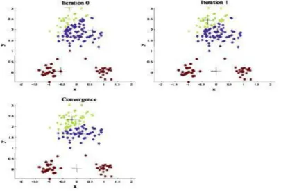
implementation is visually depicted in Fig1. Note down that each iteration requirements N × k comparisons, which
determine the time density of one iteration. The numbers of iterations obligatory for merger varies and depend on N,
but as a first cut, this algorithm can be calculated linear in the dataset size. One problem in this approach is to
decide is how to specify closest in the assignment step. The defaulting measure of closeness i the Euclidean
detachment, in which case one can gladly show that the non-negative cost purpose, The formula for centroid
locations namely,
Will reduce whenever there is an alteration in the assignment or the relocation steps, and hence junction is definite in
a predetermined number of iterations. The insatiable descent nature of k-means on a non-convex cost also
implies that the convergence is only to a local most favorable, and definitely the algorithm is typically
moderately responsive to the initial centroid locations.
In addition to being responsive to initialization, the k-means algorithm suffers from more than a few other troubles.
First survey that k-means is a restrictive case of appropriate data by a combination of k Gaussians with equal isotropic
covariance matrices “= σ 2I” when the soft assignments of data points to jumble works are unsentimental to assign
each data point exclusively to the most likely component. So it will hesitate whenever the data is not well described
by logically divided sphere shaped balls for example if there are non curved twisted clusters in the data. Problem may
be alleviated, rescaling the data to whiten it before clustering or by using expanse measure that is more suitable
for the dataset. For example information clustering in theoretic uses the KL departure to measure the distance
between two data points representing two separate chance distributions. It has been newly shown that if one
measures aloofness selecting any member of a very large class of divergences called Bergman divergences
throughout the assignment step and makes no other changes, the indispensable properties of k-means, together
with guaranteed junction, linear partition restrictions and scalability, are retained [2]. This result makes k-means
valuable for a much bigger class of datasets so long as a correct divergence is used. K means balancing
algorithm to describe non convex clusters. First clusters the data into a large number of groups using k-means.
These groups are then agglomerated into larger clusters using single link hierarchical clustering, which can
discover composite shapes. This move toward also makes the solution less perceptive to initialization, and
because the hierarchical method provides consequences at numerous resolutions, one does not require to pre
specify k either.
The cost of the optimal solution decreases with growing k till it hits zero when the number of clusters equals
the number of distinctive data-points. This makes it more difficult to (a) directly compare solutions with
different numbers of clusters and (b) to find the optimum value of k. If the preferred k is not known in advance,
one will characteristically run k-means with dissimilar values of k, and then use a suitable measure to select one
of the results. For example, a use of SAS cube-clustering-criterion, while X-means adds a complication term
which increases with k to the original cost function and then identifies the k which minimizes this adjusted cost.
Otherwise one can increasingly augment the number of clusters, in combination with a appropriate stopping
criterion. k-means achieves this by first putting all the data into a particular cluster, and then recursively
splitting the smallest amount squashed cluster into two using 2-means. The distinguished LBG algorithm [6]
used for vector quantization doubles the number of clusters till a fit code-book range is obtained. Both these
approaches thus improve the need to know k earlier. The algorithm is also perceptive to the attendance of
outliers, since mean is not a hearty guide. A preprocessing step to remove outliers can be supportive.
III. KNN: K-NEAREST NEIGHBOR CLASSIFICATION
One of the simplest and moderately insignificant classifiers is the Rote classifier, which memorizes the whole
preparation data and performs arrangement only if the attributes of the investigation entity match one of the training
examples precisely a clear disadvantage of this approach is that various test records will not be confidential because
they do not accurately competition any of the training report. A extra sophisticated approach, k-nearest neighbor
(KNN) classification [4,10], finds a cluster of k material in the training set that are bordering to the test
objective, and bases the assignment of a tag on the predominance of a exacting class in this area. There are three
key elements of this approach: a set of labeled bits and pieces, a set of stored records, a space or parallel metric
to total distance between objects, and the value of k, the number of adjacent neighbors. To order an unlabeled
the class labels of these next neighbors are then used to establish the class label of the object.
Given a training set D and a test object X = (X, Y), the algorithm computes the expanse or parallel between z
and all the training objects (X, Y) ∈ D to choose its nearest neighbor list, Dz . (X is the data of a preparation
object, while Y is its class. similarly, X is the data of the analysis object and Y is its class.)
Once the adjacent neighbor list is obtained, the test object is classified based on the common class of its nearest neighbor‟s taxonomy:
Where v is a class label, yi is the class label for the I th nearest neighbors, and I (·) is an indicator function that
returns the value 1 if its argument is true and 0 otherwise.
3.1 Issues with KNN:
There are several key issues that affect the presentation of KNN. One is the selection of k. If k is too
small, then the consequence can be susceptible to blare points. On the other hand, if k is too huge then the
district may include too many points from other classes. Another concern is the approach to combining the class
labels. The simplest technique is to take a popular vote, but this can be a difficulty if the nearest neighbors vary
extensively in their detachment and the closer neighbors more dependably specify the class of the object. A
more sophisticated approach, which is usually much fewer sensitive to the choice of k, weights each object„s
vote by its distance, where the weight issue is often taken to be the mutual of the squared expanse: wi = 1/d(x ,
xi )2 . This amounts to replacing the last step of the KNN algorithm with the following:
The option of the distance compute is another main expression. Although various measures can be used toadd
the distance between two points, the most attractive distance measure is one for which a lesser reserve between
to organize documents, then it may be better to use the cosine measure rather than Euclidean distance. Some
expanse measures can also be affected by the high dimensionality of the data. In exacting, it is well known that
the Euclidean distance consider become less discerning as the number of attributes increases. Also, attributes
may have to be scaled to prevent distance procedures from being subjugated by one of the attributes. A number
of schemes have been developed that try to compute the weights of each creature attribute based upon training
set [5].
IV. DENCLUE DENCLUE
(DENsity-based CLUstEring) is considered as a special case of the Kernel Density Estimation (KDE)
.
The KDE is a non-parametric estimation technique, which aimed to discover dense regions points. The authors of thistechnique developed this algorithm to classify large multimedia databases, because this type of database
contains large amounts of noise, and requires clustering high-dimensional feature vectors. Subsequently,
DENCLUE operates through two stages, the pre-clustering step and the clustering step as illustrated in figure 2. The first step is for constructing a map (a hyper-rectangle) of the database. This map is used to speed the calculation of the density function. As for the second step, it allows identifying clusters from highly populated
cubes(the cubes of which the number of points exceeds a threshold ξ determined in parameters), and theirs
neighbouring populated cubes. DENCLUE is based on the calculation of the influence of points between them.
The total sum of these influence functions represents the density function. There exist many influence functions,
based on the distance between two points x and y; but we will focus in this work on the Gaussian function. The
Equation (1), derived from, shows the influence function between two points x and y.
FGauss(x, y) = exp-d(x, y)2 s22, (1)
where d(x, y) is an euclidean distance between x and y, ands represents the radius of the neighbourhood
containing x.
Equation(2), extracted from13, represents the density function
.fD(x) =N_i=1fGauss(x, xi), (2)
where D represents the set of points on the database, and N its 22
x = xas shown in equation (3), presented in0, xi+1= xi+ d
∇fDGauss(x)_∇fDGauss(xii13.)_
The calculation ends when fD(xk) < fD(xk+1) with k ∈ N, then we take x*= xkas a density attractor. The points
forming a path with the density attractor, are called attracted points.
Clusters are made by taking into account the density attractors and its attracted points. The strength of this
algorithm resides in the choice of the structure with which the data are presented. A. Hinneburgand D. A. Keim
have chosen to work with the concept of hyper-rectangle. A hyper-rectangle is constituted by hypercubes. Each
hyper-cube is represented by the dimension of the feature vector points (i.e., the number of criteria) and by a
key. This structure allows to DENCLUE an easy manipulation for the data, by using the cubes keys, and
4.1.1 The Impact of the algorithm
Many of the patterns finding algorithms such as decision tree, classification rules and clustering techniques that
are frequently used in data mining have been developed in machine learning research community. Frequent
pattern and association rule mining is one of the few exceptions to this tradition. The introduction of this
technique boosted data mining research and its impact is tremendous. The algorithm is quite simple and easy to
implement. Experimenting with K medoids -like algorithm is the first thing that data miners try to do.
4.2 CURRENT AND FURTHER RESEARCH
Since K-medoids algorithm was initial introduced and as knowledge was accumulated, there have been
many attempts to develop more proficient algorithms of many item set mining. Many of them share the same idea
with K-medoids in that they spawn candidates. These include hash based system, partitioning, sampling and using
perpendicular data plan Hash based procedure can decrease the size of aspirant item sets. Each item sets are hashed
into an equivalent bucket by using a appropriate hash functions. Since a bucket can have dissimilar item sets, if its
count is less than a minimum support, these item sets in the bucket can be removed from the candidate sets. A
partitioning can be used to split the entire mining difficulty into n lesser troubles. IDs (TIDS) are connected with
each item set. With this format, mining can be performed by taking the juncture of TIDS. The support reckoning
is merely the duration of the TID set for the item set. There is no need to scan the database since TID set carries
the absolute information mandatory for computing support.
The most exceptional development more K-medoids would be a technique called FP enlargement repeated
pattern growth that succeeded in eliminating candidate invention [8]. It adopts a split and partitioning approach
by [1] compressing the database representing recurrent items into a arrangement called FP-tree (frequent pattern
tree) that retains all the essential information and [2] dividing the squashed database into a set of provisional
databases, each associated With one frequent item set and mining each one separately. It scans the database only
twice. In the first scan, all the frequent items and their support counts (frequencies) are derived and they are
sorted in the order of descending support count in each transaction. In the second scan, items in each transaction
are merged into a prefix tree and items (nodes) that appear in common in different transactions are counted.
Each node is associated with an item and its count. Nodes with the same label are linked by a pointer called
node-link. Since items are sorted in the descending order of frequency, nodes closer to the root of the prefix tree
are shared by more transactions, thus resulting in a very compact representation that stores all the necessary
frequency and extracting frequent item sets that contain the Chosen item by recursively calling itself on the
conditional FP tree. FP growth is an order of magnitude faster than the original K-medoids algorithm.
V. CONCLUSION
In this work, I have done a comparative study on the problem of clustering large dimensional datasets. We
found out that new density based clustering algorithm, named DENCLUE-IM. It was developed to improve the
capacity of the existing DEN- CLUE algorithm, to operate on the massive data, which ensures the first V
characterizing Big Data, Volume. By implementing our approach on divergent datasets. DENCLUE-IM has
proved its efficiency by outperforming the run time of DENCLUE, DENCLUE-SA and DENCLUE-GA. Our new method gives also a pretty good quality of clustering according to the three used clustering validity
metrics. We can underline that DENCLUE-IM guarantees that the three Vs of the characteristics of Big Data,
namely Volume, Variety and Veracity. Thus we proved that this approach found a trade-off between the quality of clustering and the run-time.
1) Entities forming Mobile Ad-hoc networks.
2) Aircrafts in the Airports or in the sky.
REFERENCES
[1.] J. Gantz, D. Reinsel, “The digital universe in 2020: Big data, bigger digital shadows, and biggest growth in
the far east, IDC iView: IDCAnalyze the Future” 2007 (2012) 1–16.
[2.] Yethiraj N G , “Applying Data Mining Techniques In The Field Of Agriculture And Allied Sciences” ,
International Journal of Business Intelligents ISSN: 2278-2400, Vol 01, Issue 02, December 2012.
[3.] Ramesh D, Vishnu Vardhan B., “Data Mining Techniques and Applications to Agricultural Yield Data”,
IJARCCE, Vol. 2, Issue 9, September 2013.
[4.] Mucherino, A., Papajorgji, P., &Pardalos, P. (2009), “Data mining in agriculture‖ (Vol. 34)”, Springer.
[5.] Bhagyashree Pathak and Niranjan Lal “A Survey on Clustering Methods in Data Mining”. International
Journal of Computer Applications 159(2):6-11, February 2017.