Contribution of Advanced Technology and Foreign Capital to Growth of Different Stage of Development Countries

(1)

1420

CONTRIBUTION OF ADVANCED TECHNOLOGY AND FOREIGN CAPITAL TO GROWTH OF DIFFERENT STAGE OF DEVELOPMENT COUNTRIES

Paitoon Kraipornsak

Faculty of Economics, Chulalongkorn University Bangkok, Thailand

ABSTRACT

This study determines influence of advanced technology and foreign capital on economic growth apart from contribution of the other major domestic inputs. The countries were classified into four groups; i.e., lower and lower middle income countries, upper middle income countries, non-OECD high income countries, and OECD countries. Five major factors as sources of growth in this study are domestic factors; i.e., domestic capital, labour, and human capital and supporting factors; i.e., foreign capital, and advanced technology. The long run cointegrating relation of the five major factors and its output was estimated for each group of countries. By using panel dynamic production function, most factors in the model were found significantly determining growth in all income groups. Human resources, in form of labour and human capital, were the most contributors to growth. Although all factors were found significantly contributing to growth in the OECD, at least one of the factors has not played significant role in the other three lower stages of development countries. Noticeably, both advanced technology and foreign capital were found significantly contributing to growth in all countries except for the high income Non-OECD where the advanced technology being insignificant source of growth. All five engines of growth must be put attention to play role in development of economy so that the development can be sustainable such as found all being significant factors in the case of the OECD.

Keywords: Domestic capital, Foreign capital, Human capital, Advanced technology, Country specific, Sources of growth, Cointegrating relation, Panel dynamic model.

JEL Classification: O33, O40, O50.

Contribution/ Originality

This study has used panel dynamic model that can help demonstrate the role of country

specific factor and the crucial factors determining growth in the various level of development

countries. Furthermore the study incorporated into the model human capital, foreign capital and

role of technology of which data are often unavailable and inconsistent across countries and over

periods of time.

Asian Economic and Financial Review

(2)

1421

1. INTRODUCTION

The well-known classical economic growth theory identified sources of growth into two major

factors: input growth and residual growth. The input growth consists of capital growth and labour

growth. The residual growth, or Total Factor Productivity growth, is the growth of output caused by factor other than the inputs’ growth so is named as the residual and is determined exogenously outside the system of the model.

The new endogenous growth approach has believed in roles of human capital and

accumulation of knowledge process such as research and development and technological progress

or advanced technology including externality and scale economies. The econometric method states

clearly that the omission of relevant variables in the regression equation can cause biased estimate.

In addition, possible endogenous explanatory variables included in the model can also cause the

endogenous biasedness and inconsistency of the estimation.

This study constructed the model of sources of growth by incorporating major factors

contributing to growth and estimating the model using panel data. Owing to problem of

non-stationarity of time series data of variables in the model, the dynamic model in line with the error

correction model is therefore constructed and estimated. Moreover, unobservable specific cross

country effect possibly due to differences in institutions, socioeconomic factors, culture, and

production was also incorporated into the study.

Next section will review the related literatures. It is expected to provide background on some

related studies on sources of growth. The third section described the model construction and the

data being used in the estimation. Estimation of domestic capital stock and foreign capital stock are

described. The proxies of human capital, advanced technology as well as incorporated country

specific factor being used in the study are presented in this section. Section four discussed the

estimation result and its detailed analysis in comparison across the groups of the countries. Section

five presented the conclusion.

2. LITERATURE REVIEW

The traditional Solow’s growth model put role of capital accumulation and population growth as two important conventional inputs that contribute to output growth apart from the exogenously

given residual growth being explained by technical progress (Solow, 1956; 1957). The Solow’s

growth model however requires the equilibrium condition of input elasticity equals input share and

hence constant returns to scale is a necessary condition.

To add few more important factor inputs into the sources of growth, Nelson and Phelps (1966)

explain the role of human capital and also showed that Solow residual depends on the gap of the

level of knowledge. They put emphasis on the role of education as human capital factor that can

invent and adopt new advanced technology earlier or faster so can speed up diffusion of

technology. The adoption and implementation of technology is being invented gradually at a rate

exogenously given. Therefore increase in educational attainment of labour can raise technological

(3)

1422

Mankiw et al. (1992) examined roles of physical and human capital stocks on the determinants of economic growth as factors included in the Cobb-Douglas production function. They augmented human capital as the other capital input apart from the physical capital in the Solow’s growth model. They argued that the omission of human capital input in the model can lead to biased

estimate and can explain why the roles of population growth and physical capital inputs were found

too large. Data set of selected 98 countries from Summers and Heston, the Penn World Table, was

used in the estimation. The study could indicate why some countries were rich and some countries

were poor and showed existence of conditional convergence using the traditional two input growth

model. Moreover the study found existence of non-constant returns to scale production function

and supported for the augmented human capital input into the Solow’s production function. It is

interesting to note that the Adjusted R2 or the goodness of fit of the estimated augmented production function of the OECD countries was found obviously the highest value than those of the

other 98 non-oil countries and 75 intermediate income level countries.

Human capital is also considered an important factor in the growth in Benhabib and Spiegel

(1994). When the model in which human capital associated with the growth of Total Factor

Productivity was constructed and estimated, the result showed that the human capital was

confirmed to be a significant factor determining growth. According to this paper, the human capital

can affect growth through two mechanisms: affecting the speed of technology adoption and

influencing domestically produced technology and innovation. The first mechanism was postulated

in line with Romer (1990a) that the human capital can directly influence productivity by way of

increasing capacity of the nation to innovate new appropriate technology. The second mechanism

was the one in which adapted from the model of Nelson and Phelps (1966) to allow human capital

to catch up the speed of technological innovation and diffusion. The relationship between human

capital and economic development was also tested by using long run cointegrating relation.

Enrolment rates in primary, secondary and tertiary education were found to be correlated with the

per capita GDP while the causality was tested and found that education causes GDP for primary

school and secondary school. However, for the tertiary education, it was found the reversal relation.

Human capital was considered to be an important factor of growth. The author constructed the

human capital that based on Mincerian wage equation in the previous study for Thailand

(Kraipornsak, 2009). Data of individual samples from the Labour Force Survey of the National

Statistical Office in year 1993 and 2006 was used in the estimation of the sectoral wage equations.

The human capital index was then augmented into the production function for the analysis of

growth in Thailand. The finding of the study indicated the existence of the positively long run

contribution of human capital and the Total Factor Productivity to growth in agriculture while the

physical capital input positively contribute to all sectors. The long run growth of industry can be

traded off with those of agriculture and services when allowing all sectors to interact in the growth

of the economy wide. Advanced technology has been placed a crucial role in sources of growth.

Lucas (1988) and Romer (1990b) have modeled the growth of advanced technology, or

technological progress, to depend directly on the educational level of labour, saying as human

(4)

1423 human capital is determined by incentives in the market that allocates between production and

invention that enhances the growth of technology. Therefore the role of human capital is facilitating

adoption of technology from other advance countries and creation of appropriate technology

locally.

Research and development can be considered as an investment flow that cumulates stock of the

capital investment and finally affects output as a consequence. The stock of research and

development capital was therefore accounted for another source of growth that is not easily

measurable (Griliches, 1980). He found a substantial decline in the effectiveness or the rate of

research and development capital on productivity growth during the period of the productivity

slowdown in the US during 1969 – 1977. Research and development is a process of knowledge

creation that cumulates stock of knowledge to achieve advancement in technology. Advanced

technology as a consequence of research and development investment can then be accounted for a

source of growth. It was believed that foreign direct investment can affect positively or negatively

to any economy. The positive effect of foreign direct investment has been obtained by various

possible ways such as enhancing capital formation, promoting exports, learning by doing and

technological transfer and spillover effects. The negative effect of foreign direct investment has

been mainly based on the Marxist and the dependency theories over the exploitation of and gaining

control over the host countries. In addition, there are various effects of the foreign direct investment

such as employment, growth, balance of payment, transfer of technology, and income inequality. In

overall, whether or not the foreign direct investment affects the economy positively or negatively

depends very much on how it affects the national welfare in the long run.

There have been many studies on the effects of foreign direct investment using panel data.

Recently various empirical studies on growth used panel data on the estimation of the model. The

advantage of using panel data is on its correcting for country specific differences in various factors

including institutions, culture, and socio-economic factors. Moreover, the frequent problem of

autocorrelation in the time series and the problem of heteroscedasticity in the cross sectional data

estimation can also be minimized or avoided (Hsiao, 1986). Although, to ovoid biasedness of

omitted variables in the model so country specific factor is included and fixed effect estimation is

adopted in the panel data analysis; it relies on homogeneity assumption of the different panel

country groups for a common slope. In dynamic panel data with a large time dimension, Pesaran

and Smith (1995) showed that ignorance of heterogeneity of groups of countries can create

autocorrelation of disturbances and inconsistent estimates of parameters. Average effects with

changing slopes across individual groups in dynamic panel model can be used to give consistent

estimation of mean group procedure.

De Mello (1999) studied impact of foreign direct investment on capital accumulation, Total

Factor Productivity growth and output growth and compared the results of estimation from time

series and panel data. It was found that foreign direct investment can be growth enhancing

depending on its degree of complementarity and substitution with domestic investment. If foreign

direct investment can positively affect growth, complementarity between foreign direct investment

(5)

1424 create spillovers in the production of the economy significantly so it can lead to growth of output.

By using panel data set of Summers and Heston, The Penn World Table, and divided countries into

two income level groups; i.e., OECD and non-OECD countries, the impact of foreign direct

investment should be smaller in the OECD countries group. The impact of foreign direct

investment should be smaller for the more advance countries or net exporters of foreign direct

investment. There is however evidences that many foreign direct investments occurred across

advanced economies where they are higher level of technology countries (Lucas, 1990).

The study of De Mello found mixed (positive and negative) results of foreign direct investment

impact on output growth in time series analysis in both short run and long run. Foreign direct

investment showed positively affect output growth suggesting the dominant complementary effect

between foreign direct investment and domestic investment in the fixed effect panel data estimation

after introduction of the country specific factor into the model. Under the dynamic model of foreign

direct investment, foreign capital is complementary to the domestic capital when it involves

transfer of new technology and new process and management style. Borensztein et al. (1998) also found that in sixty nine developing countries during 1970 – 1989 they needed foreign direct

investment to be as domestic absorptive capacity to enhance growth. The study revealed marginally

significant impact of foreign direct investment on growth. The foreign direct investment is

considered to be complementary to the domestic investment in the developing countries. The

magnitude of this positive effect of foreign direct investment on the economic growth however

depended on stock of human capital available in the host country.

3. MODEL AND ESTIMATION

The aggregate production function in this study consists of five major factors; i.e., domestic

capital input (KD), foreign capital input (KF), labour (L), human capital (HC), and advanced

technology (). By using panel data estimation, there is an important advantage over the time series

estimation in that the time series estimation of the standard two factor input production function

leads to possible simultaneity or endogeneity bias. The bias is caused by the relationship between

the regressors in the model and the error term since the model omits some other important variables

such as human capital and advance knowledge especially country specific difference. The high

estimates of capital elasticity coefficient well above the capital share in output found in many

studies can also be the evidence of this endogeneity bias (Young, 1995). The panel data estimation

can help correct for the endogeneity bias caused by the omission of unobservable cross-country

effects or country specific differences in institutions, socioeconomic factors, culture, and

production (Hsiao, 1986).

Recall the aggregate production function, assuming that the production function exhibits

Cobb-Douglas functional form and the technological progress is in exponential form, the aggregate

production equation is therefore written as in Equation (1) below.

 (1)

(6)

1425 Taking natural logarithmic form into Equation (1), it becomes log-linear equation as in

Equation (2) below.

 (2)

Panel data of 108 countries during 1992 – 2011 was collected and used in the estimation of the

model basically depending on availability of completeness of data on all variables in the model.

List of the countries included in the study is shown in the Appendix. Since data of some variables

used in the model estimation are not available and those available data are not consistently defined

among these countries, the study generated series to be the proxies of those variables to be used in

the model estimation. Details of each variable used in the study can be described as follows.

Y is Gross Domestic Product (GDP) measured in purchasing power parity in billion US dollars

from IMF-World Economic Outlook.

, or HTECX named in this study, is to represent the advanced technology or the stage of knowledge in each country over time. The study used the proportion of hi-tech exports on the total

exports to be the proxy of the advanced technology in the model.

KD is domestic capital stock which was estimated in the study as in Equation (3) by using the

conventional Perpetual Inventory Method (PIM) (Christensen and Jorgenson, 1969). Total

investment was divided into domestic investment and foreign investment. Capital stock was then

calculated by using the PIM equation below. Both domestic capital stock and foreign capital stock

were measured in million US dollar.

(3)

Where, Kt is capital stock, It is investment, and is depreciation rate.

KF is foreign capital stock which was calculated in the same manner as in the domestic

physical capital stock (KD) described below whereas foreign direct investment was used in place of

domestic investment in the calculation. This paper estimated the capital stock as suggested by

Berlemann and Wesselhöft (2012). Their study provides comprehensive estimations of aggregate

capital stocks for 103 countries in 2010 using the Perpetual Inventory Method in hoping for

suggestion of constructing internationally comparable datasets of capital stock. It is one of few

studies on the estimation of capital stock worldwide while it is easily extended for more countries

and for more recent years. Most available studies estimated the capital stock for the US such as

Nadiri and Prucha (1996) for the US manufacturing sector, Griliches (1980) for the US 3-digit

manufacturing industry, and Kamps (2006) for the estimated capital stock for 22 OECD countries

using investment data from the OECD Database. Kamps (2006) assumed 4.25 percent of the

depreciation rate for nonresidential assets and 1.5 percent for residential assets and 2.5 percent for

government assets. The study of Berlemann and Wesselhöft applied various approaches of the

estimation of capital stock including the unified approach. The initial capital stock (Kt0) was estimated by the following Equation (4).

(7)

1426 Where, gI is the long term growth rate of investment that is obtained by the estimation of the

equation of semi log function as in Equation (5) below. Here bj is the long term growth rate of investment. The initial period of the investment (I0) can also be obtained by this estimated equation.

(5)

The estimation results of the depreciation rate obtained by the study of Berlemann and

Wesselhöft were 3.7 percent, 0.03 percent and -1.02 percent for private non-residential fixed assets,

private residential fixed assets, and government fixed assets, respectively. Therefore, the average

rate of 1.6 percent of these three assets was assumed to be the depreciation rate in the estimation in

this study.

L is Employed labour in thousand persons from UNCTAD.

The UNDP Human Development Index combines various dimensions of human indicators

covering health, education and living standard. A minimum and a maximum for each dimension (or

goalpost) is set and each country stands in relation to these goalposts is then expressed in values

between 0 and 1 (The United Nations Development Programme). It is noted that instead of using

education enrolment rate to be the proxy of human capital as many studies did, this study

constructed the human capital index by using the international human development index of the

United Nations to make adjustment for the human capital index. In details, Human capital (HC, or

HDIAVG named in this study) was constructed by taking the human development index of the

United Nations to adjust into the number of labour to have this index reflecting its quality of human

of each country. Human development index or HDI (ranged between 0, the lowest, and 1, the

highest) that having been constructed and ranked by the United Nations was used as the parameter

to adjust the number of employed labour to be the proxy of human capital index (HDIAVG) in the

model. While higher HDI implies better human development status relatively, many more people

also means higher human capital stock. Nevertheless, the HDI was available only for the year 1990,

2000 and in each year from 2005 on. To deal with the unavailable annual data of the HDI during

1991 - 2004, the human capital index (HDIAVG) was therefore calculated by using the HDI in

1990 and 2000 for the construction of HDIAVG during 1991 – 1999 and 2000 – 2004, respectively.

The study classified the countries into four income groups mainly based on the World Bank

classifications by Gross National Income per capita as of 1st July 2013; i.e., lower and lower

middle income countries, upper middle income countries, non-OECD high income countries, and

OECD countries. Heterogeneous character across groups of countries such as natural resources,

political system, geography, weather, and religion can be considered as specific factor of countries

significantly determining different growth. In order to avoid the problem of autocorrelation of

disturbances and to gain consistent estimate, responding to Pesaran and Smith findings as

mentioned earlier, this study separately estimates the model into four income groups of countries. The study denotes this country specific factor by variable’s name of C1, C2, C3, and C4 being for the lower and lower middle income countries, the upper middle income countries, the non-OECD

(8)

1427

4. RESULTS AND DISCUSSION

In general, there are advantages of using panel data in the estimation over cross sectional units

or time series data. The case of a particular country in which too short period of time series data

available can create the problem of too small degree of freedom causing large variances of

estimated parameters and loss of power of hypothesis tests. The panel data model can be used to

avoid this small degree of freedom if under assumption of homogeneous parameter across

countries. In case of too small number of cross section or countries, the panel data can be used by

assuming country specific effect or fixed effect model. Most of all, comparing with cases of cross

sectional data, the panel data model can help avoid the possible problem of misspecification of

dynamic model biases in the estimation in case that the static model ignores the possible dynamic

adjustment of the model over time. Specifically, by inclusion of lagged dependent variable in the

dynamic model, it can control the problem of ignorance some possible omitted variables.

As almost being the case, non-stationary process is found in time series. To test for the unit

root in panel data, assuming the autoregressive process of degree 1 as written in Equation (6)

below.

it it it it

y

z

y









_ /

1 (6)

T

t

N

i

1 ,

2 ,

...,

;

2 ,

3 ,

4 ,...,

Where



; it is a stationary process;

z

_it/ is the deterministic

component and can be 0, 1, fixed effects ( i) and time trend (t).

The null hypothesis of unit root (



_i



1

) for all i is set against the alternative hypothesis of

stationary (



_i



1

). The standard unit root tests include Levin et al. (2002), Im et al. (2003) and

Fisher-type proposed by Maddala and Wu (1999) and Choi (2001).

Levin, Lin and Chu allowed heterogeneity of individual deterministic effects and

heterogeneous autocorrelation structure of the residuals and assuming homogeneous parameters in

the autoregressive process or generally so called common unit root process across cross sectional

units. It is sometimes referred to common unit root process null hypothesis. The structure of the

analysis can be written as in Equation (7) below. This panel unit root tests is more relevant for the

moderate size of the panel data.

it i i it

it

y

t

y









_₁ ₀ ₁ (7)

Where it is an invertible ARMA stationary process and is assumed to be independently distributed across individuals. The equation for this test is estimated by pooled OLS regression.

Im, Pesaran and Shin test introduces a more flexible and simple procedure of the unit root test

and allows for simultaneous stationary and non-stationary series of parameter (i) that can be different between individuals. The test also allows for autocorrelation and heterogeneity of the

dynamic error variances across groups. It is sometimes referred to individual unit root process null

(9)

1428 autocorrelated and dimensions of time and cross section are sufficiently large. The equation for this

test is estimated by balance panel data procedure. In case of autocorrelation of the residuals the test

uses Augmented Dickey Fuller t test for individual series. The rejection of the null hypothesis does

not necessary means that the unit root is rejected for all cross sectional units.

Maddala and Wu and Choi offered an alternative test following the non-parametric Fisher’s

Type test. This test is based on a combination of the probability values of the test statistics for a

unit root in each unit of cross section. While Im, Pesaran and Shin test and Fisher’s test combine

information on individual unit root tests, this test also relax the assumption of the Levin, Lin and

Chu of the same parameter (i) under alternative hypothesis. In addition, the Fisher test is based on general assumption compared to both Im, Pesaran and Shin test and Levin, Lin and Chu test. The Fisher’s test has some advantages especially that it does not require the balance panel data and is possible to use different lag lengths in the Augmented Dickey Fuller regression.

Although the data used in this study is a moderate size sample that is more relevant for the

Levin, Lin and Chu test, the other two tests were also considered and see whether there is any test

rejects the null hypothesis of the unit root. The results of the unit root tests of each variable in the

study showed that all variables are non-stationary process (Table A2 and Figure A1 in Appendix).

All series appear to be random walk processes. This suggests that there is a short-run

disequilibrium and the long-run equilibrium of the model equation. The cointegrating relation is

therefore estimated based on the approach of dynamic model. The study began by estimating the

static panel data model as in Equation (2) preliminarily using panel Least Square for all countries in

the panel data. The estimation result clearly showed that although all the estimated coefficients of

the equation were statistically significant but some of them were found to be the questionable sign

(negative sign); i.e., those of labour (ln(L)) and advanced technology (ln(HTECX)) (Equation (8)

below). In addition, the residuals of the regression line appeared to have autocorrelation problem

(Figures A2 and A3 in Appendix). This indicates possible omission of some relevant variables (i.e.,

country specific factor) in the model.

0.1317 Stat

DW 0.0000], [p

4880 . 8328

, 0738 . 224 Re

, 9567 . 0 R Adj

(-12.4874)

ln 0677 . 0

(20.5124)

(-13.7644)

(18.5365)

(41.1868)

(-77.4074)

(t)

ln 2644 . 1 ln 7632 . 0 ln

1176 . 0 ln

3545 . 0 3400 . 6 ln

2

 



 



 

 

 

F

sid SumSquare HTECX

HDIAVG L

KF KD

y

it

it it

it

(8)

The fixed effect panel data model was next estimated. The advantage of fixed effect inclusion

into the model is to help eliminate any unobservable factor assuming constant over time while

varying across countries. This implies the existence of country specific effect in the model. The

fixed effect model is written as Equation (9) below. Here, the fixed effect is denoted by i.

it i it it

it it

it

KD

KF

L

HDIAVG

HTECX

y





ln



ln



ln



ln





ln



ln

₁ ₂ ₃ ₄ (9)

The study estimated the model by introducing panel fixed effect to take account of the country

specific factor. The result is shown in Equation (10) below and country fixed effect in Table A3 in

(10)

1429 they became insignificant. The residual plot and its correlogramme were examined and found that

the residual still had some autoregressive moving average problem (Figures A4 and A5 in

Appendix), though it was little better than that of Equation (8) (as showed earlier in Figures A2 and

A3 in Appendix).

3460 . 0 ] 0000 . 0 [ 2760 . 3515 , 2555 . 23 Re , 9952 . 0 (-1.7898) ln 0059 . 0 (13.9940) (-1.4595) (27.1164) (14.7331) (-21.7745) (t) ln 8740 . 0 ln 1166 . 0 ln 1530 . 0 ln 1585 . 0 9236 . 5 ln 2             Stat DW p F sid Squared Sum AdjR HTECX HDIAVG L KF KD y it it it it it it (10)

The random effect was estimated based on Generalized Least Square. The result was shown in

Equation (11) below. Whether the fixed effects specification of cross sectional units is appropriate

or not, the test for random effect can be carried out. The essential assumption in the random effects

model is that the random effects must be uncorrelated with the explanatory variables. The study

performed the Hausman Test for random effect that is Chi-Square distribution. It was 113.9754,

which was significant, so the statistic rejected null hypothesis of independence between the residual

and the explanatory variables. The fixed effect is therefore preferable. However, the estimat ion

result similarly gave the unsatisfied residual property owing to the existence of autocorrelation.

(Figures A6 – A7 in Appendix).

3418 . 0 ], 0000 . 0 [ 8430 . 3328 1159 . 26 Re , 8982 . 0 : Statistic Weighted (-2.2493) ln 0073 . 0 (18.9696) (-6.8679) (26.2443) (19.5442) (-31.4973) (t) ln 0219 . 1 ln 3951 . 0 ln 1417 . 0 ln 1957 . 0 2378 . 5 ln 2             Stat DW p F sid Squared Sum AdjR HTECX HDIAVG L KF KD y it it it it it it (11)

The study conducted the unit root test as mentioned earlier. Since the variables used in the

model estimation were non-stationary processes; therefore, the estimate of static model as written

in Equation (2) was mis-specified dynamic biased. The unit root test of all variables could not

reject the null hypothesis of non-stationarity. The second difference series were also tested to see

whether they are non-stationary. The results of second difference series test for unit root showed to

be stationary processes therefore it indicates that all variables are integrated of order one. By being

non-stationary process of the time series variables, the appropriate equation must be constructed by

using dynamic model. The error correction mechanism type of model can be used to specify short

run disequilibrium and long run cointegrating relation between variables in the model described as

follows.

The general linear dynamic panel model specification can be written as in Equation (12)

below. The first differenced equation of the general linear dynamic model can help eliminate the

(11)

1430

it it k it P

k k i

it

Y

X

Y







_







/

1

(12)

it it

k it P

k k i

it

Y

X

Y

















_





/

1

(13)

The panel dynamic structure for the n+1 dimensional time series vector



/



, it

it X

Y and if

cointegration exists, it can be written as in Equation (14) below. The cointegrating relation between

Y and X above is assumed to be homogeneous across cross sectional units and the specification

allows for cross section specific deterministic effects.

it i it it

it

X

Z

Y





1/





/

(14)

Where

Z

_it





Z

₁/_it

,

Z

₂/_it



/ are deterministic trend regressors.

it it i it i

it

Z

X

/ ₂ ₂

22 1 /

21











(15)

And



₂_it





₂_it (16)

There are two basic estimation methods for a single cointegrating relation in general; i.e., Fully

Modified Ordinary Least Square (FMOLS) and Dynamic Ordinary Least Square (DOLS). The

study adopted DOLS method in the cointegrating relation and assumed homogeneity in the

equation1. Given cointegration is found, the panel DOLS estimator pools the data along within dimension of the panel. Kao and Chiang (2000) argued that under cointegration, DOLS is

promising in small samples and performs well so that it is consistent with the sample used in this

study. However Pedroni (2001) proposed the group mean FMOLS estimator to allow endogeneity

and autocorrelation problems to obtain consistent and asymptotically unbiased estimates.

When a panel contains large numbers of time series and cross sectional unit, the model can be

practically estimated by either separately cross sectional regressions or mean group estimator,

assuming the slope coefficients and error variances are identical. In case of pooled mean group

estimation, the long run coefficients must be constrained to be identical and the short run

coefficients and error variances can be different across groups. Pesaran et al. (1997) empirically estimated various cases including the case where it followed unit root processes and derived the

asymptotic distribution of the estimators with varying length of time period. In case of short time

period panel data, all estimators (group specific, mean group, pooled mean group, and fixed effect)

were subject to downward biased on the coefficient of lagged dependent variables.

The panel DOLS augments the panel cointegrating regression with the cross section specific

lags and leads of the difference of explanatory variable to eliminate th9 asymptotic endogeneity

1_{The study also complemented the DOLS estimation of the long run cointegrating relation by the group mean FMOLS as}

(12)

1431 and autocorrelation. The method estimates an augmented cointegrating equation as in Equation (17)

below by OLS. The equation indicates that the short run dynamic coefficients ( i) are cross section

specific.

_ 1 /

_ _

/ _

it i r

q k

k it it

it

i

i X X

Y  



 



 

 (17)

Let

/ _

k it

X





interact with cross section dummy variables to be formed as regressors (Zit

_ ) and

let

/ / _ / _ / _

, _   

 

 it it

it X Z

W , the pooled DOLS estimator can be written as Equation (18).

Moreover, Kao and Chiang showed that asymptotic distribution of the estimation is the same

as for the pooled FMOLS.









































  

 

N

i

it T

t it N

i

it T

t

it

W

Y

W

1

/ _

1 _ 1

1

/ _

1 _

^ ^

(18)

To test for cointegration, panel Pedroni’s cointegration test was performed for each of the four groups of countries as showed in Table 1 below. The test performed by lag length selection based

on SIC with lags from 0 to 2 and using Newey-West automatic bandwidth selection and Bartlett

kernel. The test can reject the null hypothesis of no unit root or, in the other word, variables are

cointegrated, especially the tests of those ADF statistics in which it allows the use of different lag

lengths in the regression equation.

To estimate for the cointegrating relation, the panel Dynamic Least Square (DOLS) estimation

method is used. It however does not allow the importance of country specific difference or cross

country heterogeneity. The study therefore took into account the country specific difference by

separately estimating the model for each of the four income groups of countries.

Table-1. Panel Cointegration Test

C1 C2 C3 C4(OECD)

Ha: common AR coefficients. (within-dimension)

Statistic [prob] Statistic [prob] Statistic [prob] Statistic [prob] Panel v-Stat. -2.0875[0.9816] -0.8909[0.8135] -0.9876[0.8383] -1.2748[0.8988] Panel -Stat. 4.7562[1.0000] 4.1675[1.0000] 3.1131[0.9991] 5.0749[1.0000] Panel PP-Stat. -1.4979[0.0671] 0.5120[0.6957] 0.5520[0.7095] 2.9231[0.9983] Panel ADF-Stat. -4.5282[0.0000] -1.8914[0.0293] -1.3986[0.0810] -1.1466[0.1258] Ha: individual AR coefficients. (between-dimension)

(13)

1432 The long run cointegrating relations for four groups of countries; i.e., one, the lower and lower

middle income countries; two, the upper middle income countries; three, the non-OECD high

income countries; and four, the OECD countries were estimated and showed in Equations (19) –

(22). The unit root tests of the residuals was also done and found that the tests reject the null

hypothesis (Table 2 – 5).

0006 . 0 , 2744 . 0 Re , 999929 . 0 AdjR (3.8081) ln 0333 . 0 (1.6332) (2.4615) (8.0343) (9.9791) (t) ln 2180 . 0 ln 4793 . 0 ln 1379 . 0 ln 3355 . 0 ln

2 _ _ _

     Variance Run Long sid Squared Sum HTECX HDIAVG L KF KD Y it it it it it it (19)

Table-2. Test for unit root of the residuals of Equation (19): country group 1 Panel unit root test

Series: RESCOINTC1

Exogenous variables: Individual effects Automatic selection of maximum lags

Automatic lag length selection based on SIC: 0 to 2

Newey-West automatic bandwidth selection and Bartlett kernel

Method Statistic Prob.**

Cross- sections Obs Null: Unit root (assumes common unit root process)

Levin, Lin & Chu t* -16.7370 0.0000 25 337

Null: Unit root (assumes individual unit root process)

Im, Pesaran and Shin W-stat -13.1846 0.0000 25 337

ADF - Fisher Chi-square 245.102 0.0000 25 337

PP - Fisher Chi-square 295.989 0.0000 25 348

** Probabilities for Fisher tests are computed using an asymptotic Chi -square distribution. All other tests assume asymptotic normality.

05 61 . 2 , 0186 . 0 Re , 999992 . 0 AdjR (8.5265) ln 1668 . 0 (7.0234) (3.6742) (7.0027) (-1.6942) (t) ln 7203 . 0 ln 8621 . 0 ln 1421 . 0 ln 2738 . 0 ln

2    

      E Variance Run Long sid Squared Sum HTECX HDIAVG L KF KD Y it it it it it it (20)

Table-3. Test for unit root of the residuals of Equation (20): country group 2 Panel unit root test

Series: RESCOINTC2

Cross-

sections Obs Null: Unit root (assumes common unit root process)

(14)

1433

Levin, Lin & Chu t* -22.2529 0.0000 17 260

0017 . 0 , 3466 . 0 Re , 999859 . 0 AdjR (-0.4825) ln 0101 . 0 (3.9122) (-0.4001) (3.5644) (4.4961) (t) ln 2750 . 1 ln 1459 . 0 ln 0970 . 0 ln 1681 . 0 ln

2   

     Variance Run Long sid Squared Sum HTECX HDIAVG L KF KD Y it it it it it it (21)

Table-4. Test for unit root of the residuals of Equation (21): country group 3 Panel unit root test

Series: RESCOINTC3 Date: 12/06/13 Time: 07:58 Sample: 1992 2011

Cross-

Levin, Lin & Chu t* -9.90936 0.0000 13 180

0007 . 0 , 3109 . 0 Re , 999962 . 0 AdjR (2.0494) ln 0.0315 (4.5748) (4.2649) (14.0390) (7.1101) (t) ln 5693 . 0 ln 6670 . 0 ln 1370 . 0 ln 1565 . 0 ln

2 _ _ _

     Variance Run Long sid Squared Sum HTECX HDIAVG L KF KD Y it it it it it

it ₍₂₂₎

The equation estimation is the part of the long run equilibrium in addition to the short run

disequilibrium dynamic part following the error correction mechanism approach. Furthermore, the

Pedroni cointegrating relation estimation extends the grouped estimator concept to DOLS

estimation by averaging over the individual cross section estimates. Therefore the goodness of fit

(R2) of this theoretical long run relation can be noticeably recorded very high as it left only very small regression error component in the calculation of R2. The study further imposed the constant returns to scale restriction into the production function equation. The Wald test for constant returns

to scale restriction was rejected in all the production function estimations (Table 6) and so it

confirmed the non-constant returns to scale production function (increasing returns as found in

(15)

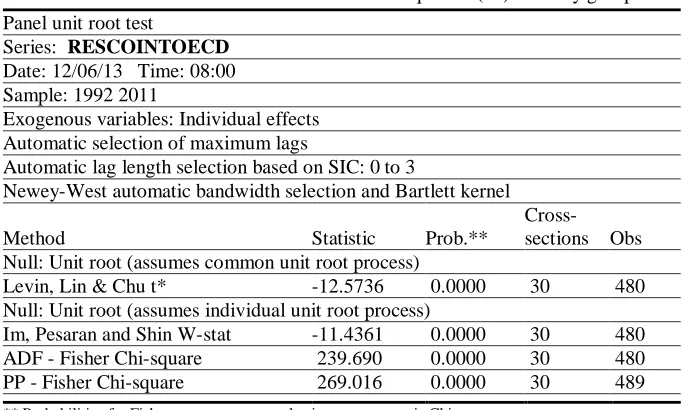
1434 Table-5. Test for unit root of the residuals of Equation (22): country group 4

Panel unit root test

Series: RESCOINTOECD Date: 12/06/13 Time: 08:00 Sample: 1992 2011

Levin, Lin & Chu t* -12.5736 0.0000 30 480

Table-6. The Wald test for constant returns to scale production function

Wald Test F-Statistic [Prob]

Lower and lower middle income countries 82.3702 [0.0000]

Upper middle income countries 25.4295 [0.0000]

Non-OECD high income countries 6.7012 [0.0098]

OECD countries 77.6517 [0.0000]

The study further examined sizes of the estimated coefficients in details in order to compare

the differences of the impacts among factors of growth. However, the sizes of coefficients of

regressors in any regression equation are not directly comparable due to their differences in their

units and their variances. The standardization adjusts the different units and different standard

errors of the variables just like the Z-score statistic so that these standardized coefficients unit-less

scores can be comparable across variables as written in Equation (23) below.

(23)

Where = standardized coefficient of the jth explanatory variable = coefficient of the jth explanatory variable

SEj = standard error of the jth explanatory variable

SEy = standard error of y variable

Table 7 below shows the sizes of the standardized coefficients of variables in each group of

country. Since the production function was a log-linear equation, the coefficient of variable means

its elasticity of output or its factor share in the equilibrium condition. The result in Table 7 thus

clearly indicated that either labour or human capital or both forms of human factor are the factors

contributing most to the output growth in the four income level groups of countries. Note also that

labour was found to be the least (and insignificant) contributor to growth for the non-OECD high

(16)

1435 domestic capital was found to be the least (and insignificant) contributor to growth for the upper

middle income countries (group 2) where many of them are new emerging or rapidly growing

countries. This insignificant negative impact of domestic capital on growth can imply that there

was substitution or displacement of stronger effect of foreign capital and its weaker effect of

domestic capital on growth in such countries. Although all factors were found significantly

contributing to growth in the OECD, at least one of the factors has not played significant role in the

other three lower stages of development countries. Both advanced technology and foreign capital

significantly contribute to growth in all countries except the high income Non-OECD where the

advanced technology being insignificant source of growth.

Table-7. The standardized coefficients of the production function

Coefficient of C1 C2 C3 C4

L 0.0490 0.0872 -0.0352 0.0377

HDIAVG 0.0153 0.0319 0.2750 0.0256

KD 0.0059 -0.0191 0.0042 0.0012

KF 0.0012 0.0012 0.0017 0.0005

HTECX 0.0002 0.0014 -0.0001 0.0002

Source: Author’s calculation

The finding of significant long run contribution of human capital to economic growth in most

income countries, except in the lower and lower middle income countries, is consistently found as

in many previous studies. In addition, the advanced technology was found to be a crucial factor to

growth except for the high income non-OECD. These two findings confirm the essential role of

human capital and advanced technology in promoting sustainable economic growth especially in

the upper middle income countries and the advanced high income OECD. Likewise, foreign capital

was found to play significant contribution to growth in all countries from the rich to the poor. This

confirms the conventional hypothesis of the role of capital accumulation in economic growth

particularly that of foreign capital. A policy implication on these findings indicates importance of

advanced technology and foreign capital which are crucial supporting factors apart from investment

in human capital to sustain economic growth in the long run. Most of all, all the mentioned five

engines of growth must be placed attention to play role in development of economy so that the

development can become of great success such as found all being significant factors in the case of

the OECD. Certainly, the country specific factor cannot simply be changed though it is also found

important.

5. CONCLUSION

Apart from the conventional role of capital accumulation and population growth in economic

growth; human capital, foreign capital, and advanced technology are also the other important

(17)

1436 Panel data of 108 countries during 1992 – 2011 was collected and used in the estimation of the

aggregate production function. For the disaggregate model, the study classified the countries into

four groups; i.e., lower and lower middle income countries, upper middle income countries,

non-OECD high income countries, and non-OECD countries based on the World Bank income

classifications by GNI per capita. The study generated indices as proxies for some variables used

in the model estimation. Since data for physical capital in many countries in the study is incomplete, Perpetual Inventory Method (PIM) was used to estimate the countries’ domestic and foreign physical capital stocks. Human capital was estimated and used as the proxy by taking the

Human Development Index of the United Nations to make adjustment to number of workers for

each country. The ratio of hi-tech export to the total export of goods was used to be the proxy of

advanced level of technology.

Since all variables in the model are found to be non-stationary processes and be integrated of

order one, the dynamic model is appropriate and the cointegrating relation of the production

function was estimated. By using panel dynamic least square method, the long run cointegrating

relations of the production function were estimated for the four groups of countries separately. This

separated equation estimation can also help avoid the biased problem due to the possible omission

of country specific factor as the separately estimated equations can be considered as each

individual or independent function. This study showed that the pooled mean group panel dynamic

model estimation for each group of countries provided better result than the panel fixed effect

model. As a part of the superiority of the panel dynamic model estimated separately by each

income group to be accounted for each country specific factor, the pooled mean group dynamic

model allows short run dynamic to differ across countries while the aggregate panel fixed effect

model does not have this dynamic effect.All the estimated production functions were found

exhibiting non-constant returns to scale and were consistent with most findings of the new

endogenous growth theory. Interestingly, all coefficients of factors were found significant for the OECD’s long run production function. At least one of those factors of growth was found insignificant for the other three lower income groups. The advanced technology and foreign capital

can be the supporting factors and thus the OECD growth is better sustainable than the other

countries. The finding indicates importance of advanced technology and foreign capital which are

crucial factors apart from investment in human capital to sustain economic growth in the long run.

All the five engines of growth were found being significant factors in the case of the successful

OECD therefore a policy must be placed attention to these five factors to fully play their roles on

growth.

Besides, these estimation results are in line with the endogenous growth approach. The human

capital and the advancement of knowledge, or named in this study the advanced technology, are the

two important endogenous factors of growth and must be included in explanation of the

conventional Total Factor Productivity growth, previously considered as the exogenously given

residual growth. As the result, the residual growth is found insignificant or it is approaching zero

(18)

1437

REFERENCES

Benhabib, J. and M.M. Spiegel, 1994. The role of human capital in economic development: Evidence from

aggregate cross country data. Journal of Monetary Economics, 34(2): 143-173.

Berlemann, M. and J.E. Wesselhöft, 2012. Estimating aggregate capital stocks using the perpetual inventory

method: New empirical evidence for 103 countries. Diskussionspapierreihe Working Paper Series

No. 125. Hamburg, Germany: Helmut Schmidt University, Department of Economics.

Borensztein, E., J.D. Gregorio and J.W. Lee, 1998. How does foreign direct investment affect growth?. NBER

Working Paper No. 5057, Cambridge.

Choi, I., 2001. Unit root tests for panel data. Journal of International Money and Finance, 20(2): 249-272.

Christensen, L.R. and D.W. Jorgenson, 1969. The measurement of U.S. real capital input, 1929-67. Review of

Income and Wealth, 15(4): 293 - 320.

De Mello, J.L.R., 1999. Foreign direct investment-led growth: Evidence from time series and panel data.

Oxford Economic Papers, 51(1): 133-151.

Griliches, Z., 1980. R&D and the productivity slowdown. NBER Working Paper Series No. 434. Cambridge.

Hsiao, C., 1986. Analysis of panel data. Cambridge: Cambridge University Press.

Im, K.S., M.H. Pesaran and Y. Shin, 2003. Testing for unit roots in heterogeneous panels. Journal of

Econometrics, 115(1): 53-74.

Kamps, C., 2006. New estimates of government net capital stocks for 22 OECD countries 1960 – 2001. IMF

Staff Paper, 53(1): 120 – 150.

Kao, C. and M.H. Chiang, 2000. On the estimation and inference of a cointegrated regression in panel data. In

Baltagi, B.H. et al. eds. Nonstationary panels, panel cointegration and dynamic panels, 15.

Amsterdam: Elsevier. pp: 179-222.

Kraipornsak, P., 2009. Roles of human capital and total factor productivity growth as sources of growth:

Empirical investigation in Thailand. International Business & Economics Research Journal, 8(12):

37-52. Available from http://journals.cluteonline.com/index.php/IBER/article/view/3196/3244. Levin, A., C.F. Lin and C.S.J. Chu, 2002. Unit root tests in panel data: Asymptotic and finite sample

properties. Journal of Econometrics, 108(1): 1-24.

Lucas, R., 1988. On the mechanics of economic development. Journal of Monetary Economics, 22(1): 3-42. Lucas, R., 1990. Why doesn’t capital flow from rich to poor countries? American Economic Review, 80(2):

92 – 96.

Maddala, G. and S. Wu, 1999. A comparative study of unit root tests and a new simple test. Oxford Bulletin of

Economics and Statistics, 61(S1): 631-652.

Mankiw, M.G., D. Romer and D.N. Weil, 1992. A contribution to the empiric of economic growth. Quarterly

Journal of Economics, 107(2): 407 – 437.

Nadiri, M.I. and L.R. Prucha, 1996. Estimation of the depreciation rate of physical and R&D capital in the

U.S. total manufacturing sector. Economic Inquiry, 34(1): 43 – 56.

Nelson, R. and E. Phelps, 1966. Investment in humans, technological diffusion, and economic growth.

American Economic Review, 56(1/2): 69-75.

Pedroni, P., 2001. Purchasing power parity tests in cointegrated panels. Review of Economics and Statistics,

(19)

1438

Pesaran, M.H., Y. Shin and R.P. Smith, 1997. Pooled estimation of long-run relationships in dynamic

heterogenous panels. DAE working papers amalgamated Series No. 9721, University of Cambridge.

Pesaran, M.H. and R. Smith, 1995. Estimating long-run relationships from dynamic heterogeneous panels.

Journal of Econometrics, 68(1): 79-113.

Romer, P., 1990a. Endogenous technological change. Journal of Political Economy, 98(5): S71-S102.

Romer, P., 1990b. Human capital and growth: Theory and evidence. Carnegie Rochester Conference Series on

Public Policy, 32(1): 251-286.

Solow, R., 1956. A contribution to the theory of economic growth. Quarterly Journal of Economics, 70(1): 65 – 94.

Solow, R., 1957. Technical change and the aggregate production function. Review of Economics and

Statistics, 39(3): 312 – 320.

The United Nations Development Programme. Human development report, various issues. Available from:

http://hdr.undp.org/en/statistics/hdi.

Young, A., 1995. The tyranny of numbers: Confronting the statistical realities of the East Asian growth

experience. Quarterly Journal of Economics, 110(3): 640 – 680.

APPENDIX

As of 1 July 2013, the World Bank income classifications by GNI per capita are as follows: • Low income: $1,035 or less

• Lower middle income: $1,036 to $4,085 • Upper middle income: $4,086 to $12,615 • High income: $12,616 or more

Appendix-1.

Table-A1. List of the countries included in the study

(20)

1439 Table-A2. Test for panel unit root

Panel unit root test Series: lnY Sample: 1992 2011

Cross-

Levin, Lin & Chu t* -1.34632 0.0891 109 1969

Im, Pesaran and Shin W-stat 10.5067 1.0000 109 1969

Panel unit root test Series: lnKD

Cross-

Levin, Lin & Chu t* 6.61186 1.0000 108 1838

** Probabilities for Fisher tests are computed using an asymptotic Chi-square distribution. All other tests assume asymptotic normality.

Panel unit root test Series: lnKF

Cross-

Levin, Lin & Chu t* 2.26494 0.9882 108 1875 Null: Unit root (assumes individual unit root process)

Im, Pesaran and Shin W-stat 15.4172 1.0000 108 1875 ADF - Fisher Chi-square 137.395 1.0000 108 1875 PP - Fisher Chi-square 31.0000 1.0000 108 2025

(21)

1440 Panel unit root test

Series: lnL

Exogenous variables: None

Automatic selection of maximum lags

Cross-

Levin, Lin & Chu t* 27.1507 1.0000 109 1985

Panel unit root test: Summary Series: lnHDIAVG

Levin, Lin & Chu t* -0.49219 0.3113 109 2055

Panel unit root test Series: lnHTECX

Exogenous variables: Individual effects, individual linear trends Automatic selection of maximum lags

Cross-

Levin, Lin & Chu t* -6.58995 0.0000 107 1715

Breitung t-stat 4.74294 1.0000 107 1608

(22)

1441 Table-A3. Country fixed effect

Country Effect Country Effect Country Effect Country Effect

ALB -0.051723 EGY -0.118681 LAT 0.219227 SAU 0.864067

ALG 0.189144 ELS 0.138111 LEB 0.269898 SIN 0.383350

ARG -0.234324 EST 0.226432 LIT 0.315831 SLK 0.288783

AME -0.336875 FIN 0.446690 MAL -1.098180 SLN 0.430264

AUS 0.171635 FRA 0.253092 MAY -0.122445 SAF 0.213056

AUT 0.509618 GEO -0.666923 MAU 0.275740 SPA 0.251122

AZE -0.411226 GER 0.113099 MEX 0.029313 SLA -0.545041

BAH 0.558381 GRE 0.419888 MOL -0.860204 SUD -0.279379

BAN -0.979745 GUA -0.120938 MON -0.282612 SWE 0.291848

BEL 0.079830 HON -0.185630 MOR -0.396387 SWI 0.190712

BEG 0.223984 HOK -0.106272 NEP -0.719319 SYR 0.169853

BOL -0.430102 HUN 0.239419 NET 0.197941 TAJ -0.934786

BOT 0.146613 ICE 0.673376 NEW 0.040867 TAN -0.988154

BRA -0.215584 IND -0.469333 NIC -0.169729 THA -0.646395

BRU 0.998680 INN -0.732903 NIR -0.652862 TRI 0.086940

BUL 0.247494 IRA 0.650182 NOR 0.609617 TUN -0.167959

CAM -0.910534 IRE 0.342754 OMA 0.751708 TUR 0.317470

CAN 0.249379 ISR 0.475244 PAK -0.305521 UGA -0.683005

CHI -0.101160 ITA 0.430061 PAN -0.213310 UK 0.202770

CHN -1.022496 JAM -0.152117 PAR -0.308637 UKR -0.433052

COL 0.005928 JAP -0.066856 PER -0.200575 UAE 0.992904

COS -0.013239 JOR -0.203652 PHI -0.742052 URU -0.029914

CRO 0.631168 KAZ -0.195778 POL 0.239432 USA 0.212959

CYP 0.344226 KEN -0.654190 POR 0.118393 VEN 0.142447

CZE 0.258095 KOR 0.234784 QAT 1.486632 VIE -1.069250

DEN 0.275603 KUW 1.725792 ROM 0.149837 YEM -0.036514

ECU -0.071428 KYR -0.752796 RUS 0.083042 ZAM -1.124330

Figure-A1. Correlogramme of Series

Series lnY

Sample: 1992 2011

Included observations: 2169

Autocorrelation Partial Correlation AC PAC Q-Sta... Pro...

(23)

1442 Series lnKD

Series lnKF

Series lnL Sample: 1992 2011

1 0.942 0.942 1893.8 0.000

2 0.886 -0.007 3570.7 0.000

3 0.830 -0.034 5041.8 0.000

4 0.774 -0.021 6324.4 0.000

5 0.720 -0.023 7433.9 0.000

6 0.666 -0.026 8384.8 0.000

7 0.613 -0.026 9190.8 0.000

8 0.561 -0.027 9865.3 0.000

9 0.509 -0.030 10421. 0.000

10 0.457 -0.031 10870. 0.000

11 0.406 -0.031 11224. 0.000

12 0.356 -0.031 11496. 0.000

Sample: 1992 2011

1 0.932 0.932 1854.3 0.000

2 0.862 -0.048 3441.2 0.000

3 0.791 -0.042 4779.3 0.000

4 0.721 -0.036 5891.0 0.000

5 0.652 -0.028 6802.0 0.000

6 0.586 -0.024 7538.0 0.000

7 0.523 -0.018 8124.9 0.000

8 0.464 -0.015 8586.3 0.000

9 0.408 -0.019 8942.3 0.000

10 0.354 -0.020 9210.8 0.000

11 0.303 -0.020 9407.4 0.000

12 0.255 -0.017 9546.6 0.000

Sample: 1992 2011 Included observations: 2178

Autocorrelation Partial Correlation AC PAC Q-Sta... Prob