Application of computational fluid dynamics on cavitation in
journal bearings
Marco Riedel1,a, Marcus Schmidt2, Peter Reinke1, Matthias Nobis1, and Marcel Redlich2
1 West Saxon University of Applied Science Zwickau, Dr.-Friedrichsring 2A, 08056 Zwickau (Germany) 2 Forschungs- und Transferzentrum e.V., POB 20 10 37, 08012 Zwickau (Germany)
Abstract. Journal bearings are applied in internal combustion engines due to their favourable wearing quality and operating characteristics. Under certain operating conditions damage of the journal bearing can occur caused by cavitation. The cavitation reduces the load capacity and leads to material erosion. Experimental investigations of cavitating flows in dimension of real journal bearing are difficult to realize or almost impossible caused by the small gap and transient flow conditions. Therefore numerical simulation is a very helpful engineering tool to research the cavitation behaviour. The CFD-Code OpenFOAM is used to analyse the flow field inside the bearing. The numerical cavitation model based on a bubble dynamic approach and requires necessary initial parameter for the calculation, such as nuclei bubble diameter, the number of nuclei and two empirical constants. The first part of this paper shows the influence of these parameters on the solution. For the adjustment of the parameters an experiment of Jakobsson et.al. [1] was used to validate the numerical flow model. The parameters have been varied according to the method Design of Experiments (DoE). With a defined model equation the parameters determined, to identify the parameter for CFD-calculations in comparison to the experimental values. The second part of the paper presents investigations on different geometrical changes in the bearing geometry. The effect of these geometrical changes on cavitation was compared with experimental results from Wollfarth [2] and Garner et.al. [3].
1 Introduction
The hydrodynamic journal bearing is an established me-chanical element in internal combustion engines. It stands out by the fact of bear high loads, nearly wearless and low noise operating conditions. The simple design and the low priced manufacturing are further advantages. Like in other hydrodynamic applications cavitation is still a problem in journal bearings. Caused by the cavitation, erosion of the surface can occur and that can result in the breakdown of the bearing. To prevent the damage of the journal bearing it is necessary to have knowledge about the cause of cav-itation. Only if vapour appears in the flow, cavitation can occur. Therefore investigation of the flow in the bearing with considering of vaporisation is necessary.
For that investigations the computational fluid dynamics (CFD) is used. Cavitation is founded by three dimensional (3D) effects. Therefore the simulations are realised with the 3D-CFD-Code OpenFOAM. This is a excellent tool due to the free availability and the open solver code. The advantage of the numerical simulation is that every detail of the flow can be obtained. Experiments cannot offer this diversity. On the other hand an experiment is necessary to validate the numerical results. One step at the preparation of the simulation is the grid generation. Therefore special
a e-mail:
regions has to be considered. A further step in the prepara-tion is the adaptaprepara-tion of the solver on the flow condiprepara-tions in a journal bearing geometry. Therefore the experiment of Jakobsson et.al. [1] is choosen to simulate different pa-rameter variations according to the method Design of Ex-periments (DoE). The configuration with the best results is used for a further simulation at the journal bearing of Wollfarth [2]. In the secound part of the paper changes in the geometry of the end of the groove and a different shape of the feed hole run out are tested at the journal bearing of [2].
2 Numerical Model
2.1 Geometrical Parameters
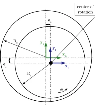
The geometrical parameters of a journal bearing are given in this section. In figure1 the different dimensions are il-lustrated. The inner cylinder with the radiusR1is rotating withωaround the center of rotation. The fixed outer cylin-der with the radiusR2stands still.
The displacement of the inner cylinder is considered by the two eccentricitiesexandey. Other important values can be calculate from the parameters given in figure1 by the following equations 1 to 5.
yA
xA
yI
xI
ex
ey
R1
R2
center of rotation
ω
Fig. 1schematic illustration of the principal journal bearing geometry
H0 =R2−R1 (1)
U1=ω·R1 (2)
Re=Ψ·R1·U1
ν (3)
Ψ= H0
R1
(4)
εx,y= ex,y
H0
(5)
2.2 Mathematical model
The numerical solver is based on the finite-volume method. For a typical journal bearing of an internal combustion en-gine the Reynoldsnumbers is calculatedRe≈35 [4]. That means that the flow is laminar. Furthermore the flow is isothermal since the bubble collaps is not considered. So the system of partial differential equations is reduced to the three dimensional conservation equations for mass (eq. 6) and momentum (eq. 7).
∂ρ
∂t +∇ ·(ρu)=0 (6)
∂ρu
∂t +(u· ∇)u=ρ g− ∇p+μ∇
2u (7)
To consider a secound phase and the phase change a trans-port equation have to be solved. This transtrans-port equation is given in eq. 8.
∂α
∂t +∇ ·(αu)+∇ ·[α(1−α)uα]=
˙ m++m˙−
ρl
(8)
The volume fractionαdepends on the volume of liquid Vland the volume of vapourVv in a cell and is calculated with eq. 9.
α= Vl
Vl+Vv
(9)
The third term in eq. 8 is only significant at the inter-face between the liquid and vapour phase. Ifα=1 (liquid) orα=0 (vapour) the term disappears. The velocity of the compression from the interface is given by the valueuα. The source term on the right side of eq. 8 describes va-porisation ˙m+and condensation ˙m−. For this source term a bubble dynamic approach according to Sauer [5] is used. The transfered mass is calculated by eq. 10.
˙
m=ρl·ρv
ρ ·
3αNuc
R ·(1−αNuc)·sign[pv−p]·R˙
·⎧⎪⎨⎪⎩CC,i f sign[pv−p]=−1 CV,i f sign[pv−p]=1
(10)
The densityρand the viscosityνare calculated as a mix-ture which depends onα, see eq. 11 and eq. 12.
ρ=ρlα+ρv(1−α) (11)
ν=νlα+νv(1−α) (12)
The ratio of vapourαNuc depends on the radius of the nucleiRand the number of nuclein0.
αNuc=
4 3πR
3n 0 1+43 πR3n
0
(13)
For the bubble dynamic approach the velocity of the nuclei wall ˙Ris necessary. Therefore the simplified Rayleigh-Plesset equation 14 is used.
˙ R=
2 3 ·
|pv−p|
ρl
(14)
To adapt the solver for special cases two dimensionless constantsCC andCV are used. They have a linear influ-ence on the transfered mass of vapour or liquid. Close to the interface between vapour and liquid the eq. 7 is ex-tended by the surface tensionσ. The momentum equation in such regions is given in eq. 15.
∂ρu
∂t +(u· ∇)u=ρ g−σ
1
R n− ∇p+μ∇
2u (15)
2.3 Grid Generation
Fig. 2numerical grid for the simulations
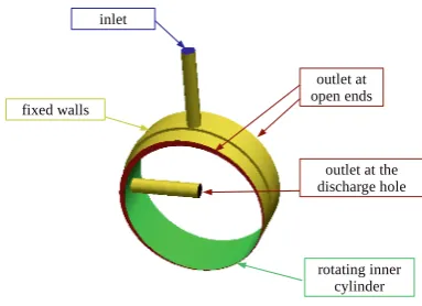
Fig. 3boundaries at the hole numerical model
Table 1boundary conditions for the simulation of the experi-ment from Jakobsson et.al. [1]
vol. fraction pressure velocity
inner cylinder ∇α=0 ∇p=0 ω=48,1s−1 outer cylinder ∇α=0 ∇p=0 u=(0 0 0)T
open ends α=1 p=1bar ∇ ·u=0
2.4 Boundary Conditions
Cause of the two experiments, different boundaries are de-fined. For the simulation of the experiment from Jakobsson et.al. [1] only the fixed outer cylinder, the rotating inner cylinder and the outlet at the open ends has to be consid-ered. At the simulation of the experiment from Wollfarth [2] furthermore an inlet at the feedhole, the outlet at the discharge hole, the fixed walls from feedhole, groove and discharge hole has to be considered. All these boundaries are shown in figure 3. The boundary conditions for both experiments are listed in table 1 and 2
2.5 Procedure
In the real life the movement of the shaft in the bearing is very complex. It rotates around the centre axis, moves on a trajectory and is affected by the deformation of the housing. The consideration of all these effects leads to a complex CFD-Model resulting in long real time for the
Table 2boundary conditions for the simulation of the experi-ment from Wollfarth [2]
vol. fraction pressure velocity
inlet α=1 p=15bar u= f(p) fixed walls ∇α=0 ∇p=0 u=(0 0 0)T
inner cylinder ∇α=0 ∇p=0 ω=210s−1 outlets α=1 p=1bar ∇ ·u=0
Table 3identified values for different parameters parameter value/range
vapour pressure pv=0,1Pa
surface tension σ=0,0265N/m
liquid density ρl=800. . .870kg/m3
liquid viscosity νl=1. . .2·106m2/s
vapour density ρv=9,8kg/m3 vapour viscosity νv=0,418·106m2/s
simulation. A moderate time for the simulation is impor-tant for practical analysis. Therefore an alternative solu-tion were found. In the first step the flow field is calculated with a steady-state solver with one fluid and without phase change. Here equation 6 and 7 are solved. The resulting values for pressure and velocity in every cell are the initial solution for the transient solution. The time for the simula-tion is the necessary time for turning the shaft about 2◦. It is assumed that the position of the shaft (exandey) is known. For this short time the moving of the shaft on a trajectory and the deformation of the housing is neglected. The grid of the transient solution is the same like in the steady-state case. With this approach the special case of flow cavitation can be analised. This special type of cavitation in a jour-nal bearing is founded by the deflection of the flow and a higher velocity caused by a smaller passage to pass by the flow. In this case the position of the discharge hole plays an important role and has to be considered.
3 Adjustment of the Parameters
3.1 Selection of the Parameters
In the equations 8 to 15 two constants and eight properties are included. For the liquid phase the values for density
3.2 Design of Experiments
To identify the relationship and the effect between diff er-ent variables it is often necessary to perform a lot of exper-iments or simulations. Because of limited time and money the number of experiments or simulations are also limited. To get the most knowledge from the simulations the DoE is a good method. A model equation describes the relation-ship between the result and the variables. In the most cases a linear approach with interactions between the variables is sufficient to describe the relationship [8]. An example for a linear model with interactions is given in eq. 16.
φ=a0+
m
i=1
ai·χi+ m
i=1 i+1
j=1
ai j·χi·χj. . .
+ak·χi·χj·. . .·χm
(16)
In the Jakobsson experiment the attributeφis the cavitation lengthlcav. The valuesχi. . . χmare functions from the un-known variables. This functions are unun-known and the best way to identify these functions is to test different functions with considering the effect on the attributelcav. The values
a0. . .akare the parameters of the model equation. These
parameters should be identidied after the run of the experi-mental design. Equation 16 could also be written in matrix form. The parametervektor a¯ can than be determined by eq. 17.
¯ a=F¯T
·F¯ −1·F¯T
·φ¯ (17)
At a two level design (every variable is tested at two dif-ferent settings) the effect of the different variables can be calculated from the difference of the mean values at the high and low level. A large effect indicates that these vari-able has a large influence on the result. The effect can also be determined at interactions of variables.
3.3 Testing the Approach
The approach is verified with statistical tests. First the va-lidity of the model equation is tested with regard to the experimental design. Then the determination of the regres-sion is tested. For the validity of the model equation the simple coefficient of correlationrop has to be determined, eq. 18.
rop= sop so·sp
(18)
The covariance sopobtains to the measured length of the simulation and the length calculated from the model equa-tion.
sop= 1 N−1
N
i=1
(φi,Meas−φ¯Meas)·(φi,Mod−φ¯Mod) (19)
The standard deviationssoandspare also calculated from the length of the simulation and the calculated length.
so=
1 N−1
N
i=1
(φi,Meas−φ¯Meas)2 (20)
sp=
1 N−1
N
i=1
(φi,Mod−φ¯Mod)2 (21)
0 0.02 0.04 0.06 0.08 0.1 0.12 0.14 0.16
ABD ABC B AB ABCD C A BD BCD ACD CD BC D AC n0 x CV
standardised effect
n0 x dNuc x CC x CV
dNuc x CV
n0 x dNuc x CV
n0 x dNuc x CC
dNuc
n0 x dNuc
CC
n0
dNuc x CC x CV
n0 x CC x CV
CC x CV
dNuc x CC
CV
n0 x CC
n0 x CV
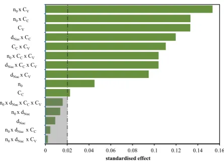
Fig. 4standardised effect of every variable and interaction
With the simple coefficient of correlation and the number of simulationsNthe following comparison has to be done:
rop
1−r2 op
· √N−2>t1−λ,f. (22)
The valuet1−λ,f is the percentile from the Student- distri-bution with the probability of error λ and the degree of freedom f = N −1. A typical value for the probability of error isλ=0,05. If the comparison 22 is accepted the model equation is validated for the tested configuration of variables. The secound test is the determination of the re-gression. Therefore the multiple coefficient of correlation rχiφhas to be determined. For every parameter of the model equation a single multiple coefficient of correlation exists and is calculated with eq. 23.
rχiφ=
1− det|S¯| s2
i ·det|S¯ii|
(23)
The valuedet|S¯|is the determinant of the covariance ma-trix,s2
i is the variance of the respective parameter anddet|S¯ii| is the subdeterminant of the covariance matrix. The subde-terminant is formed by removing from rowiand columni. With every multiple coefficient of correlation the following comparison has to be done:
r2 χiφ 1−r2 χiφ
·N−k
k−1 >F1−λ,f1,f2 (24)
Herekstands for the number of parameters. The percentile of the Fisher-distribution F1−λ,f1,f2 depends on the
proba-bility of error λ and the degree of freedom f1 = k−1 and f2 = N−k. If the comparison 24 is accepted, the re-lationship between the variable and the model equation is confirmed.
3.4 Analysis of the System
Table 4adjustment levels for the unknown variables
parameter high level low level
number of nuclei n0,H =1010 n0,L=108
diameter of nuclei dNuc,H=10μm dNuc,L=2μm
constant for condensation CC,H=1 CC,L=0,1
constant for vaporisation CV,H=10 CV,L=1
4 it is shown that the diameter of the nuclei has an influ-ence smaller than 2% and can be neglected. Also the inter-actionsn0·dNuc·CC·CV,n0·dNuc·CC,n0·dNuc·CV and n0·dNuchave small influence on the result so they are also neglected. Every other variable and interaction is received, so eq. 25 is the linear model equation for the given case.
φModell,1=a0+a1·χ1+a2·χ3+a3·χ4+. . .
. . .+a4·χ1χ3+a5·χ1χ4+a6·χ2χ3. . .
. . .+a7·χ2χ4+a8·χ3χ4+a9·χ1χ3χ4. . .
. . .+a10·χ2χ3χ4
(25)
The following relationship were tested and proved as the best:
– χ1 =log10(n0),
– χ2 =log10(dNuc),
– χ3 =log10(CC),
– χ4 =log10(CV).
In the case of four variables a full factorial design of the simulation runs is acceptable. That means for four vari-ables on two adjustment levels, 24 = 16 tests have to be performed. From older simulations some experience about the coarse range of the values is present. The high and low levels for every variable is given in table 4.
With eq. 17 the parametervektor is determined. The statistical test 22 indicates with more than 95% probabil-ity that the model equation 25 is correct. Comparison 24 indicates for eight parameters also more than 95% proba-bility of correctness. Only the parametersa6 anda7have more than 90% probability of correctness, but this seems to be also ok. With model equation 25 a cavitation length lCav =96,86mmwere determined with the following ad-justment:
– n0=1010,
– nNuc=2μm,
– CC=0,179,
– CV =5,58.
The cavitation length of the appendant simulation islCav= 109,4 mmand is to large. To improve the quality of the model equation first the full linear model equation with every interaction is used. This does not improve the re-sult. Further steps with different model equations of sec-ound order don‘t show an advantage. To solve that prob-lem a model equation with higher order terms is neces-sary. Therefore more simulations have to be done to train a neuronal network. The effort for that is very extensive and should not be carried out in the given case. Alternatively the simulation is chosen with the most closest cavitation length (the value islCav =97,2mm) as reference. The ac-cording settings are as follows:
– n0=108,
end of the groove
damage at the bearing surface
moving of the shaft
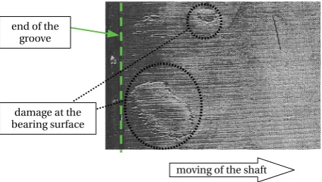
Fig. 5damage of the bearing surface downstream the end of the groove
vapour at the wall of the bearing
Fig. 6vapour region downstream the end of the groove in the simulation
– nNuc =2μm,
– CC =0,1,
– CV =1.
4 Results
4.1 Validation of the Model
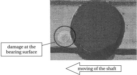
In the first run the prepared model shall be validated with experimental data. Therefore the experiment from Woll-farth [2] is the reference. In this experiment the damage of the bearing surface is a indicator for the existence of cavi-tation respectively vapour at the bearing surface. In figure 5 the damage of the bearing surface is shown downstream the end of the groove. Therefore the discharge hole is placed at an angle 90◦downstream the feedhole. This is because the deflection of the flow is founded in the presence of the dis-charge hole at this region. In figure 6 the vapour region in the simulation is close to the surface of the bearing. This indicates the possibility of cavitation at the surface. The comparison of the cavitation regions in figure 5 with the vapour region in figure 6 shows a good agreement.
the feedhole. The related illustration from the simulation is shown in figure 8. Also in this case the vapour region is in good agreement with the damaged region at the bear-ing surface. The comparison between the numerical results and the damages from the experiment is very good. The conclusion is that the numerical solver gives a plausible solution for the flow cavitation in a journal bearing.
damage at the bearing surface
moving of the shaft
Fig. 7damage of the bearing surface downstream the feedhole
vapour at the wall of the
bearing
Fig. 8vapour region downstream the feedhole in the simulation
4.2 Investigation in Geometrical Changes
After the validation of the model were done, the influence of different geometrical changes shall be tested. In the first series of simulations the effect of different shapes of the end of the groove is tested. A flow efficient shape should prevent the behaviour of cavitation. In Wollfarth [2] inves-tigations on six different shapes were done. Three chamfer ends and three rounded ends were tested. The smoothest intersection should indicate the fewest affinity of cavita-tion. The vapour regions of the simulation is shown in ure 9 and figure 10. A qualitative analysis is shown in fig-ure 11 where the volume of vapour of every shape is related to the unmachined shape. It is obvious that the amount of vapour decreases with smoother groove ends. In case of the smoothest intersection (14◦chamfer and rounded end with R = 20 mm) the amount of vapour increases compared with the next smoothest intersection. The reason for that is founded in the high velocity in this region. The veloc-ity of the original shape, the 14◦chamfer and the rounded end withR=20mmis shown in figure 12. Caused by the smaller gap between the groove and the discharge hole the velocity increases and the pressure decreases. It is obvious that the main stream is more aligned to the wall and that the
chamfer 14° chamfer 20°
chamfer 45° unmachined
Fig. 9three chamfer ends in comparison with the unmachined end of the groove
unmachined
R 10 mm R 20 mm R 5 mm
Fig. 10three rounded ends in comparison with the unmachined end of the groove
org.
45°
20°
14°
R5
R10
R20
0 0.25 0.5 0.75 1
volume of vapour related to the unmachined
sh
a
p
e
of
t
h
e
g
roo
ve en
d
Fig. 11relative volume of vapour related to the unmachined groove end
velocity is higher than in the original case. If the velocity is high enough the pressure underrun the vapour pressure and then the amount of vapour increases.
unmachined
R 20 mm Chamfer 14°
Fig. 12velocity in a planar cut of different shapes of the groove end
amount of vapour at the wall increases
Fig. 13velocity in a planar cut of different shapes of the groove end
is not equal to the width of the groove. In every other sim-ulation the diameter of the feedhole and the discharge hole are equal to the width of the groove. To consider the cham-fer a little modification at the model were done. This leads to the difference between the diameter and the width of the groove. However the simulation illustrates the decreasing risk of cavitation in the case of the chamfered intersection.
5 Conclusion and Outlook
In this work the possibility of simulating cavitating flow in a journal bearing geometry is shown. The constants and unknown properties for the specific numerical solver were found. With this settings the validation between the numer-ical results and the experimental data has been done. The results are satisfying. Furthermore the expected improve-ment of changes in geometrical details were shown in the simulation. This is a further reason to trust the results of the CFD simulation.
In further works the numerical gridgeneration can be im-proved. Details like chamfers, different shapes of the groove etc. should be optional adapted to the model. Otherwise other geometrical changes like different widths of the groove, heights of the groove and relative bearing clearances could be observed.
Nomenclature
ai model constant
¯
a parametervektor
CC constant for condensation CV constant for vaporisation dNuc diameter of the nuclei,μm e eccentricity,m
¯
F variationmatrix
F1−λ,f1,f2 percentile of the Fisher-distribution
f degree of freedom of the Student-distribution f1 first degree of freedom of the
Fisher-distribution
f2 first degree of freedom of the Fisher-distribution
g gravity acceleration, 9,81m/s2 H0 bearing clearance,m
k number of model constants lCav length of the cavitation area,m
˙
m+ mass flow of transfered vapour,kg/(s m3) ˙
m− mass flow of transfered liquid,kg/(s m3)
N number of tests
n normal vector
n0 number of nuclei, 1/m3
p pressure,Pa
R radius of the nuclei,m R1 radius of the inner cylinder,m R2 radius of the outer cylinder,m
˙
R velocity of the bubble wall,m/s
Re Reynoldsnumber
rop simple coefficient of correlation rχi,φ muliple coefficient of correlation
¯
S covariance matrix
s2
i variance of the valuei
so standard deviation of the measurement sop covariance betweeb the measurement and the
model
sp standard deviation of the model sign signum function
t time,s
t1−λ,f percentile of the Student-distribution U1 velocity in circumference direction,m/s
u vector of velocity,m/s
uα velocity of the compression of the interface, m/s
V volume,m3
α volume fraction
αNuc ratio of vapour
ε relative eccentricity
λ probability of error
μ dynamic viscosity,Pa s
ν kinematic viscosity,m2/s
ρ density,kg/m3
σ surface tension,N/m
φ result of model equation respectively measure-ment
χ transformed variable
Ψ relative bearing clearance
ω angular velocity, 1/s
Indices
l liquid v vapour x,y,z coordinates
References
1. B. Jakobsson, L. Floberg, Transactions of Chalmers University of Technology190, (1957) pages 6-116 2. M. Wollfarth,Experimentelle Untersuchung der
Kavi-tationserosion im Gleitlager(PhD Thesis, University of Karlsruhe), (1995)
3. D.R. Garner, R.D. James, J.F. Warriner, Journal of En-gineering for Power102, (1980) pages 847-857
4. M. Riedel, Numerische Untersuchung von Kavitation-seffekten in Radialgleitlagern(Master Thesis, University of Applied Science Zwickau), (2013)
5. J. Sauer, Instation¨ar kavitierende Str¨omungen - Ein neues Modell basierend auf Front Capturing (VoF) und Blasendynamik (PhD Thesis, University of Karlsruhe), (2000)
6. Verein Deutscher Ingenieure (VDI); VDI-W¨armeatlas (Berlin), (2006)
7. Akron University, USA; ull.chemistry.uakron. edu/erd/Chemicals/4000/2639.html (2013)