Collision of a small bubble with a large falling particle

(1)

Collision of a small bubble with a large falling particle

Jiri Vejrazka1,a_{, Martin Hubicka}2_{, and Pavlina Basarova}2

1 _{Institute of Chemical Process Fundamentals, 165 02 Praha 6, Czech Republic}

2 _{Prague Institute of Chemical Technology, Department of Chemical Engineering, 166 28 Praha 6, Czech Republic.}

Abstract. The motion of a tiny bubble (<1mm) in a neighborhood of a solid sphere falling through a liquid is studied. A model assuming irrotational ﬂow around the sphere and spherical bubble shape is provided; this model is validated by comparison with the experiment. The model can be further simpliﬁed by neglecting inertial forces, which are negligible in present experiments. Results of the model are provided also for the opposite limit, in which the inertial forces are dominating the bubble motion.

1 Introduction

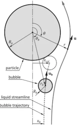
Motivated by applications of separation of various plas-tic materials by ﬂotation during their recycling, we study the behavior of a tiny (De<1mm) bubble rising in water, which encounters a larger spherical particle falling through the liquid (with velocityUpin order of few cm/s). The aim is to determine, what are the conditions under which the bubble touches the particle’s surface. Basically, all bub-bles, which are initially in a distancex0(see ﬁgure 1) smaller

than some limiting valuexg collide with the particle sur-face, whereas bubbles with x0 > xg do not collide. The

aim hence reduces in an eﬀort of obtaining an expression for the maximum collision distancexg.

In paper by Hubicka et al.[1], we have experimentally investigated the collision. We have provided a model for the bubble motion, which was based on expressing hydro-dynamic forces acting on the bubble. We have also shown that for studied conditions of small particle velocity (which

a _e-mail:_{[email protected]}

Fig. 1.Studied conﬁguration and symbols.

are typical for practical conditions), the model can be fur-ther simpliﬁed by considering only the drag and buoyancy forces. In this conference contribution, we will summarize our previous work [1]. In addition, we will show results of the model for the hypothetical opposite case, in which the bubble motion is dominated only by inertial forces, and the drag and buoyancy can be neglected.

2 Experimental observations

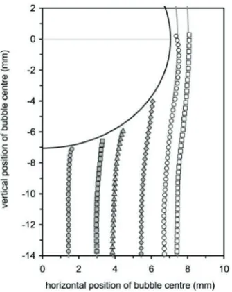
In experiments, a single bubble (0.5 to 0.8 mm in diam-eter) was created in a controlled manner [2] in a glass cell (height 50 cm, width 8 cm and depth 6 cm). A glass ball (14.1 mm in diameter) was fixed to a traversing de-vice, which displaced it downward with a velocity of 5 or 10 cm/s. A high-speed camera (Redlake Motion Pro) was moved by another traversing device with the same velocity as the glass particle. Movies of the bubble motion around the particle (recorded with a rate of 500 frames per second, resolution 1280x1024 pixels and scale 14μm) were ana-lyzed using NIS-Elements software; this analysis provided data about the bubble size and its trajectory. Experiments were repeated with several bubble sizes, two particle veloc-ities and two different working fluids. For each operating condition, several trajectories differing in the initial bubble position x0 were recorded, leading to a set of

experimen-tal trajectories, whose example is shown in ﬁgure 2. More details about experiments are provided in [1].

A remarkable behavior observed in experiments is the linear dependence of the bubble position at the instant of collision with the particle surface, on the initial position,

xcol=kx0, as it is illustrated in ﬁgure 3.

3 Model

In this contribution, we consider three different models for the bubble motion. Thefull modelsolves the bubble trajec-tory in the frame of reference, which moves with the par-ticle (figure 1). This model is simplified by omitting some terms, leading to eithernon-inertialorinviscidmodels. DOI: 10.1051/

C

Owned by the authors, published by EDP Sciences, 2014

/2 01

epjconf 4 6 702125

(2)

Fig. 3.Observed dependence of the radial distancexcolat the time of collision with the particle, on the initial positionx0of the bubble.

Data for pure water, particle velocity 50 mm/s (a-d) and 100 mm/s (e-h).

Fig. 2.Example of observed and computed trajectories of bubble. Velocity of the ball is 50 mm/s, bubble diameter 0.596 mm, pure water.

3.1 Full model

The full model assumes that the liquid motion around the sphere is not aﬀected by the bubble, and is modeled by an irrotational ﬂow. Such an assumption is reasonable if the Reynolds number of the sphere is high enough,

Rep=2 ρUpRp

μ 1, (1)

and valuesRe >100 are generally suﬃcient (ρandμare the liquid density and viscosity). It is also assumed that the impulse related with the bubble motion is smaller than the impulse related with the motion of the sphere (ρR3

bUb ρR3

pUp). The assumption of irrotational ﬂow holds reason-ably only upstream the sphere (i.e. in its lower part), but is

not justified downstream the sphere, where the flow sepa-rates. Another assumption is that the bubble remains spher-ical. In low-viscosity fluids, this assumption is satisfied if the Weber number of the bubble remains small during its motion,

We=2ρRb|ub−u|

2

σ 1, (2)

whereσis the surface tension. This assumptions is the ﬁrst to be unsatisﬁed in the present works. On other hand, the present paper is valid also for motion of some light spher-ical particles around a larger moving particle; the assump-tion about the Weber umber is not required in such a case. The bubble trajectory is obtained by solving an equa-tion for bubble moequa-tion. This equaequa-tion is written as a bal-ance of forces, which act on the bubble. Those forces in-clude thebuoyancy,drag,added-mass,inertiaandlift,

Fb+Fd+Fam+FI+FL=0. (3)

The added-mass force Fam is proportional to the bubble acceleration, while other forces are either constant or de-pendent on the bubble velocity. The balance (3) is hence a diﬀerential equation of second order (for each position component). Detailed expressions of considered forces are provided in [1].

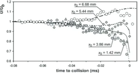
The force balance (3) is not complete, as some forces (e.g. the history force [3]) are neglected. The model com-pares well with the experimental data, however. This is apparent from ﬁgure 2, in which experimental trajectories (points) are drawn above results of the full model (lines, mostly hidden below the symbols). Furthermore, the ve-locity evolution of the bubble is also captured correctly, as it is apparent from ﬁgure 4, where modeled and experi-mental velocity of the bubble are compared.

(3)

contact with the particle surface. This is mostly due to the inertial forceFIin front of the bubble.

It is noted that a similar model for motion of small particles around larger bubbles was presented recently by Huang et al. [6].

3.2 Non-inertial model

A remarkable behavior [1] observed in experiments (and in results of the computations by the full model for low parti-cle velocities) is the linear dependence of the radial bubble position at the instant of collision with the particle surface, on the initial radial position,xcol = kx0. This simple

de-pendence is easily explained if we consider for the bubble velocityubat each instant

ub=u+ub,0, (4)

whereu is the local liquid velocity in the location of the bubble andub,0is the velocity of bubble rise in a still liq-uid. Equation (4) follows from (3) if only buoyancyFband dragFd are considered, whereasFam,FI andFL are ne-glected. The trajectory of the bubble is then easily derived via the stream function. The stream functionψof ﬂuid par-ticles moving around the sphere is given by

ψ=1 2

⎛ ⎜⎜⎜⎜⎜ ⎝1−R

3

p

r3 ⎞ ⎟⎟⎟⎟⎟

⎠Upr2sin2θ. (5)

Thebubble trajectory functionψbis computed. This func-tion is constant along the bubble trajectory, and is hence analogous to stream function ψ, which is constant along the trajectory of the liquid. It is expressed by adding the term 1₂Ub,0r2sin2θtoψ; this term corresponds to the

mo-tion with constant velocityUb,0 aligned with the particle

axis. We hence obtain

ψb= 1 2

Up+Ub,0 ⎡ ⎢⎢⎢⎢⎢

⎢⎣1− R

3

p

1+Ub,0/Up r_b3

⎤ ⎥⎥⎥⎥⎥

⎥⎦r_b2sin2θ (6)

Note thatψbhas the same form as the stream functionψof the ﬂow around a sphere, but the velocity is diﬀerent (Up+

Ub), as well as the sphere radius (Rp(1+Ub,0/Up)−1/3). The collision occurs when the bubble distance from the particle center isrb=Rp+Rp. Using (6), we can now easily derive an expression for the collision positionxcol, which is

Fig. 4.Comparison of the bubble velocity computed using the full model and experimental data.

found (in agreement with experiments) in the formxcol =

kx0, where the constantkis

k=

⎡ ⎢⎢⎢⎢⎢

⎢⎢⎢⎣1− R

3

p

1+Ub,0/Up

Rp+Rb

3 ⎤ ⎥⎥⎥⎥⎥ ⎥⎥⎥⎦

−1 2

. (7)

The maximum initial distancexg, for which the bubble just

touches the particle surface, is easily determined as

xg=

Rp+Rb

k . (8)

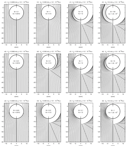
The presented non-inertial model is basically a com-bination of the classical models of Sutherland [4] and of Flint and Howarth [5], applied to the case of moving bub-bles instead of settling particles, for which those models have been developed. Its results are also shown in Figure 5 (gray lines in the left parts of the trajectory maps, which are frequently overlapped by black lines). For the results seen in the second row of ﬁgure 5 (results for water), the non-inertial model predicts correctly the bubble trajectory for velocities up to 10 cm/s, which is the case of experi-ments [1].

3.3 Inviscid model

The remaining terms of the motion equation (3) are studied by neglecting the buoyancy and drag forces,FbandFd. All remaining forces (Fam,FIandFL) follow from the inertia of the liquid, and such a model is hence purely inertial. The rising motion of the bubble is now assured by imposing the velocityUb,0 via initial conditions; because the drag and buoyancy are neglected, the initial velocity is maintained up to the interaction with the particle.

The resulting trajectories are shown in figure 5 in the right halves of the trajectory maps. For small particle ve-locity, the bubbles continue due to its inertia (represented by the added-mass forceFam) straight ahead and hits the particle with unchanged velocity (figure 5a). At higher ve-locitiesUp, the bubble trajectory is deflected due to the in-ertial forceFIacting on the bubble (figures 5b2 and 5c2). This inertial force prevents the bubbles to come close to the particle surface. As the particle velocity is increased, the distance, in/to which the bubbles are deflected, is in-creasing (compare figures 5b2 and 5c2); however, at high velocities, this distance is then increasing only very slowly (figures 5c2 and 5e2) in consequence of the character of the inertial forceFI, which decreases with the distance from the particle as∼r−4_.

The inertial model shows another feature, which might be easily overlooked in ﬁgure 5: close the particle’s equator (θ=90◦), the inertial forceFIattracts the bubbles toward the particle. This is seen from the curvature of trajecto-ries of the bubble, which bend toward the particle’s surface close to the particle’s equator.

(4)

−10 −5 0 5 10 −30 −25 −20 −15 −10 −5 0 5 x(mm)

a1) U_p = 0.0093 m/s, μ = 9.1 ⋅ 10−5Pa.s

St = 0.1 Ac = 0.0012

−10 −5 0 5 10

References

1. M. Hubicka, P. Basarova J. Vejrazka, Int. J. Mineral Proc.121,21 (2013)
2. J. Vejrazka, M. Fujasova, P. Stanovsky, M. Ruzicka, J. Drahos, Fluid Dyn. Res.40,521 (2008)
3. J. Magnaudet, I. Eames, Annu. Rev. Fluid Mech. 32, 659 (2000)
4. K. L. Sutherland, J. Phys. Chem.52, 394 (1948) 5. L. R. Flint, W. J. Howarth, Chem. Eng. Sci.26, 1155