Experimental determination of the yield locus of anisotropic metal sheets using digital image correlation

University of Windsor University of Windsor

Scholarship at UWindsor

Scholarship at UWindsor

Electronic Theses and Dissertations Theses, Dissertations, and Major Papers

2009

Experimental determination of the yield locus of anisotropic metal

Experimental determination of the yield locus of anisotropic metal

sheets using digital image correlation

sheets using digital image correlation

Neil D. Turton University of Windsor

Follow this and additional works at: https://scholar.uwindsor.ca/etd

Recommended Citation Recommended Citation

Turton, Neil D., "Experimental determination of the yield locus of anisotropic metal sheets using digital image correlation" (2009). Electronic Theses and Dissertations. 7930.

https://scholar.uwindsor.ca/etd/7930

This online database contains the full-text of PhD dissertations and Masters’ theses of University of Windsor students from 1954 forward. These documents are made available for personal study and research purposes only, in accordance with the Canadian Copyright Act and the Creative Commons license—CC BY-NC-ND (Attribution, Non-Commercial, No Derivative Works). Under this license, works must always be attributed to the copyright holder (original author), cannot be used for any commercial purposes, and may not be altered. Any other use would require the permission of the copyright holder. Students may inquire about withdrawing their dissertation and/or thesis from this database. For additional inquiries, please contact the repository administrator via email

NOTE TO USERS

This reproduction is the best copy available.

EXPERIMENTAL DETERMINATION OF THE YIELD

LOCUS OF ANISOTROPIC METAL SHEETS USING

DIGITAL IMAGE CORRELATION

By

Neil D. Turton

A Thesis

Submitted to the Faculty of Graduate Studies through Mechanical, Automotive, & Materials Engineering

in Partial Fulfillment of the Requirements for the Degree of Master of Applied Science at the

University of Windsor

Windsor, Ontario, Canada

2009

1*1

Published Heritage Branch

395 Wellington Street OttawaONK1A0N4 Canada

Bibliotheque et Archives Canada

Direction du

Patrimoine de I'edition

395, rue Wellington Ottawa ON K1A 0N4 Canada

Your file Votre reference ISBN: 978-0-494-57613-7 Our file Notre reference ISBN: 978-0-494-57613-7

NOTICE: AVIS:

The author has granted a

non-exclusive license allowing Library and Archives Canada to reproduce, publish, archive, preserve, conserve, communicate to the public by

telecommunication or on the Internet, loan, distribute and sell theses

worldwide, for commercial or non-commercial purposes, in microform, paper, electronic and/or any other formats.

L'auteur a accorde une licence non exclusive permettant a la Bibliotheque et Archives Canada de reproduire, publier, archiver, sauvegarder, conserver, transmettre au public par telecommunication ou par Plnternet, preter, distribuer et vendre des theses partout dans le monde, a des fins commerciales ou autres, sur support microforme, papier, electronique et/ou autres formats.

The author retains copyright ownership and moral rights in this thesis. Neither the thesis nor substantial extracts from it may be printed or otherwise reproduced without the author's permission.

L'auteur conserve la propriete du droit d'auteur et des droits moraux qui protege cette these. Ni la these ni des extra its substantiels de celle-ci ne doivent etre imprimes ou autrement

reproduits sans son autorisation.

In compliance with the Canadian Privacy Act some supporting forms may have been removed from this thesis.

Conformement a la lot canadienne sur la protection de la vie privee, quelques

formulaires secondaires ont ete enleves de cette these.

While these forms may be included in the document page count, their removal does not represent any loss of content from the thesis.

Bien que ces formulaires aient inclus dans la pagination, il n'y aura aucun contenu manquant.

Author's Declaration of Originality

I hereby certify that I am the sole author of this thesis and that no part of this thesis has been

published or submitted for publication.

I certify that, to the best of my knowledge, my thesis does not infringe upon anyone's copyright

nor violate any proprietary rights and that any ideas, techniques, quotations, or any other

material from the work of other people included in my thesis, published or otherwise, are fully

acknowledged in accordance with the standard referencing practices. Furthermore, to the

extent that I have included copyrighted material that surpasses the bounds of fair dealing within

the meaning of the Canada Copyright Act, I certify that I have obtained a written permission

from the copyright owner(s) to include such material(s) in my thesis and have included copies of

such copyright clearances to my appendix.

I declare that this is a true copy of my thesis, including any final revisions, as approved by my

thesis committee and the Graduate Studies office, and that this thesis has not been submitted

Abstract

The focus of this research was to determine the yielding and work hardening behaviour of two

anisotropic steel sheets (DP600 and HSLA). Uniaxial tension and compression tests were

performed in the rolling and transverse directions and at 45 degrees to the rolling direction for

each sheet. Plane-strain tension tests were carried out along the rolling and transverse

directions. Digital image correlation was used to determine the strain distribution throughout

the gauge region.

The stress-strain response of the plane-strain tension specimen was estimated through a

comparison of the experimental and numerically predicted load-strain response.

Yield stresses in uniaxial tension were obtained for various yield offsets, and R-values were

obtained, allowing for the anisotropy of each steel sheet to be determined. Yield data was also

obtained in plane-strain and equibiaxial tension, pure shear, and uniaxial compression for

corresponding values of plastic work per unit volume from the stress-strain response.

Hill's 1948 R-based and stress-based yield criteria, Hill's 1979 planar-isotropic yield criterion and

Barlat's Yld2000-2d yield function were evaluated at each value of plastic work per unit volume,

and compared against the experimental yield data obtained.

A low degree of anisotropy was noted for both materials. While all yield functions provided

similar results for DP600, it was noted that Hill's 1948 R-based, criterion and Hill's 1979 yield

criterion were unable to accurately predict material behaviour for all yield offsets for HSLA. It

was found that Barlat's Yld2000-2d provided the most accurate representation of the

Acknowledgements

I would like to express my sincere appreciation and gratitude to Dr. D. E. Green for his guidance

and support over the course of this study. His assistance over the course of my research has

been invaluable.

I would also like to thank my committee members for their support, especially Dr. W. Altenhof

for his assistance with the development of the numerical model.

The assistance of the laboratory technicians, Mr. A. Jenner, Mr. L. Pop, Mr. M. St Louis, and

Mr. P. Seguin is greatly appreciated. The assistance of Mr. A. Jenner in specimen preparation is

especially appreciated.

Finally, I would like to thank my fellow researchers, including Mr. A. Taherizadeh, Mr. A. Ghaei,

Table of Contents

AUTHOR'S DECLARATION OF ORIGINALITY lii

ABSTRACT iv

DEDICATION v

ACKNOWLEDGEMENTS vi

LIST OF TABLES. x

LIST OF FIGURES xii

LIST OF SYMBOLS xvii

1 . INTRODUCTION.... 1

2 . LITERATURE REVIEW 5

2.1 PLASTIC ANISOTROPIC COEFFICIENT 5

2.2 ANISOTROPIC YIELD FUNCTIONS 6

2.2.1 Hill's 1948 criterion 7

2.2.2 Hill's 1979 criterion 8

2.2.3 YLD2000-2d .... 9

2.3 EXPERIMENTAL DETERMINATION OF THE YIELD LOCUS 11

2.3.1 Plane-strain tension 12

2.3.2 Equibiaxial tension 13

2.3.3 Uniaxial compression 15

2.3.4 Pure shear 17

2.4 DIGITAL IMAGE CORRELATION 19

3 . EXPERIMENTAL PROCEDURES 21

3.1 TEST SPECIMENS 21

3.1.2 Specimen geometries 22

3.1.3 Specimen preparation 25

3.2 TESTING PROCEDURES 27

3.2.1 Testing equipment 27

3.2.2 System calibration 28

3.2.3 Strain measurement accuracy 30

3.2.4 Testing procedure 31

3.2.5 Numerical analysis of plane-strain tension tests 34

3.3 OUTSOURCED TESTS , ...36

3.4 ANALYSIS OF DATA 37

4 . RESULTS AND DISCUSSION 39

4.1 UNIAXIAL TENSION RESULTS 39

4.1.1 DP600 39

4.1.2 HSLA 43

4.2 NUMERICAL PREDICTION OF PLANE-STRAIN TENSION BEHAVIOUR 47

4.2.1 DP600 48

4.2.2 HSLA 54

4.3 EXPERIMENTAL PLANE-STRAIN TENSION RESULTS 61

4.3.1 DP600 61

4.3.2 HSLA 65

4.4 UNIAXIAL COMPRESSION RESULTS 70

4.5 OUTSOURCED TEST RESULTS 72

4.6 YIELD FUNCTIONS 76

4.6.1 DP600 88

5 . CONCLUSION ₉₉

APPENDIX A. ARAMIS SPECIFICATIONS 101

APPENDIX B. PLANE-STRAIN ANALYSIS 104

APPENDIX C. OUTSOURCED STRESS-STRAIN RESULTS 113

REFERENCES.... 120

List of Tables

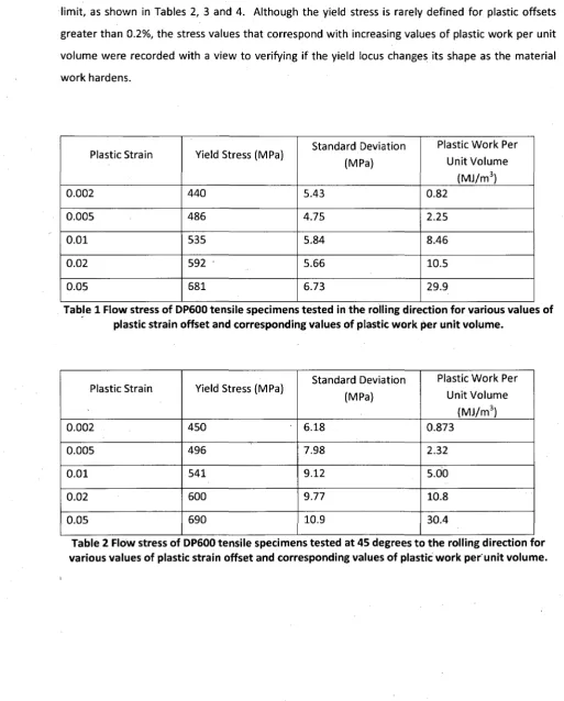
Table 1 Flow stress of DP600 tensile specimens tested in the rolling direction for various values

of plastic strain offset and corresponding values of plastic work per unit volume 42

Table 2 Flow stress of DP600 tensile specimens tested at 45 degrees to the rolling direction for

various values of plastic strain offset and corresponding values of plastic work per unit volume 42

Table 3 Flow stress of DP600 tensile specimens tested at 90 degrees to the rolling direction for

various values of plastic strain offset and corresponding values of plastic work per unit volume 43

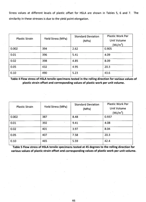
Table 4 Flow stress of HSLA tensile specimens tested in the rolling direction for various values of

plastic strain offset and corresponding values of plastic work per unit volume 46

Table 5 Flow stress of HSLA tensile specimens tested at 45 degrees to the rolling direction for

various values of plastic strain offset and corresponding values of plastic work per unit volume 46

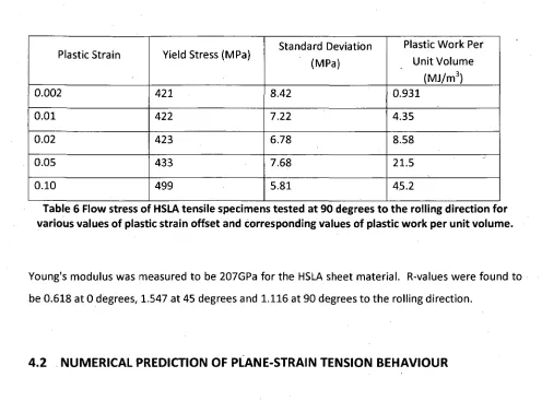
Table 6 Flow stress of HSLA tensile specimens tested at 90 degrees to the rolling direction for

various values of plastic strain offset and corresponding values of plastic work per unit volume 47

Table 7 Flow stress in DP600 plane-strain specimens loaded in the sheet rolling direction 64

Table 8 Flow stress in DP600 plane-strain specimens loaded in the sheet transverse direction 65

Table 9 Flow stress in HSLA plane-strain specimens loaded in the sheet rolling direction 69

Table 10 Flow stress in HSLA plane-strain specimens loaded in the sheet transverse direction 70

Table 11 Flow stress in DP600 uniaxial compression specimens loaded in the sheet rolling

direction •. 71

Table 12 Flow stress in DP600 uniaxial compression specimens loaded at 45 degrees to the sheet

rolling direction 72

Table 13 Flow stress in DP600 uniaxial compression specimens loaded at 90 degrees to the sheet

rolling direction '. '. 72

Table 14 Flow stress in DP600 uniaxial compression specimens loaded in the sheet rolling

direction 73

Table 15 Flow stress in DP600 uniaxial compression specimens loaded at 90 degrees to the sheet

rolling direction 73

Table 16 Flow stress in HSLA uniaxial compression specimens loaded in the sheet rolling

Table 17 Flow stress in HSLA uniaxial compression specimens loaded at 90 degrees to the sheet

rolling direction 74

Table 18 Equibiaxial tension stress coefficients 74

Table 19 Flow stress in DP600 equibiaxial tension specimens 75

Table 20 Flow stress in HSLA equibiaxial tension specimens 75

Table 21 DP600-Simple shear yield values 76

Table 22 HSLA - Simple shear yield values ...76

Table 23 Anisotropy coefficients for Hill's 1948 stress-based yield function 88

Table 24 Anisotropy coefficients for Barlat's Yld2000-2d .89

Table 25 Anisotropy coefficients for Hill's 1948 stress-based yield function ...94

Table 26 Anisotropy coefficients for Barlat's Yld2000-2d 94

List of Figures

Figure 1.1 Schematic of advanced high strength steels, high strength steels, and mild steels 2

Figure 2.1 Schematic of cold rolling process showing rolling (X) and transverse (Y) directions 5

Figure 2.2 Effect of m coefficient on yield function 9

Figure 2.3 Yield locus representing key points for measurement 11

Figure 2.4 Strain distribution of major and minor strain in plane-strain test 12

Figure 2.5 a) Wagoner's 'H' design for strain specimen b) Wagoner's 'B' design for

plane-strain specimen 13

Figure 2.6 Cruciform specimen 14

Figure 2.7 Methods for compression testing 17

Figure 2.8 Geometry of pure shear specimen 18

Figure 2.9 Simple shear device developed at the Universite de Bretagne-Sud 18

Figure 3.1 Uniaxial tension specimen corresponding to ASTM Standard E8M 23

Figure 3.2 Uniaxial compression specimen 24

Figure 3.3 Plane-strain specimen 25

Figure 3.4 Plane-strain specimen prepared for analysis using ARAMIS system 26

Figure 3.5 Plane-strain tension clamps ....28

Figure 3.6 Calibration panel.. 29

Figure 3.7 (A) Location of ARAMIS strain measurements on specimen (B) Stress-strain profiles

from ARAMIS and extensometer 31

Figure 3.8 Experimental set-up for uniaxial tension test with ARAMIS cameras 32

Figure 3.9 Experimental set-up for plane-strain tension tests ...33

Figure 3.10 Experimental set-up for uniaxial compression tests 34

Figure 3.11 Numerical model of plane strain specimen ..35

Figure 4.1 Engineering stress-strain behaviour of DP600 in uniaxial tension 40

Figure 4.3 Distribution of the true major strains in the gauge area of DP600 uniaxial tension

specimens 41

Figure 4.4 Engineering stress-strain behaviour of HSLA in uniaxial tension 44

Figure 4.5 True stress-true strain behaviour of HSLA in uniaxial tension 44

Figure 4.6 Distribution of the true major strains in the gauge area of HSLA uniaxial tension

specimens 45

Figure 4.7 Load-Stress behaviour of DP600 specimens in plane-strain tension obtained from

numerical analysis 48

Figure 4.8 Numerical prediction of stress-strain behaviour for DP600 specimen subjected to

plane-strain tension in the rolling direction before and after scaling 49

Figure 4.9 Estimated stress-strain behaviour of DP600 in plane-strain tension 50

Figure 4.10 Comparison of the plane-strain behaviour of DP600 in the rolling direction as predicted by the Wagoner analysis method and by scaling the curves obtained from finite

element simulation 51

Figure 4.11 Comparison of the plane-strain behaviour of DP600 at 90 degrees to the rolling direction as predicted by the Wagoner analysis method and by scaling the curves obtained from

finite element simulation 52

Figure 4.12 (A) Major and (a) minor strain distribution in DP600 plane-strain specimen predicted

with LS-Dyna 53

Figure 4.13 Distribution of major and minor true strains computed across the width of the gauge

for numerical model of plane-strain DP600 specimen loaded in the rolling direction. 54

Figure 4.14 Load-stress behaviour of HSLA specimens in plane-strain tension obtained from

numerical analysis 55

Figure 4.15 Numerical results for HSLA specimen in rolling direction before and after scaling in

rolling direction 56

Figure 4.16 Estimated true stress-true strain behaviour of HSLA in plane-strain tension 57

Figure 4.17 Comparison of the plane-strain behaviour of HSLA in the rolling direction as predicted by the Wagoner analysis method and by scaling the curves obtained from finite

element simulation 58

Figure 4.18 Comparison of the plane-strain behaviour of HSLA at 90 degrees to the rolling direction as predicted by the Wagoner analysis method and by scaling the curves obtained from

Figure 4.19 (A) Major and (a) minor strain distribution in DP600 plane-strain specimen predicted

with LS-Dyna ...: 59

Figure 4.20 Distribution of axial major and minor true strains computed across the width of the

gauge for numerical model of plane-strain HSLA specimen loaded in the rolling direction 60

Figure 4.21 Distribution of axial major and minor engineering strains measured across the width

of the gauge for plane-strain DP600 specimens loaded in the rolling direction 61

Figure 4.22 Distribution of axial major and minor engineering strains measured across the width

of the gauge for plane-strain DP600 specimens loaded at 90 degrees to the rolling direction 62

Figure 4.23 Distribution of (A-D) axial and (a-d) transverse true strains measured in the gauge

area of DP600 plane-strain specimens 64

Figure 4.24 Distribution of axial major and minor engineering strains measured across the width

of the gauge for plane-strain HSLA specimens loaded in the rolling direction 66

Figure 4.25 Distribution of axial major and minor engineering strains measured across the width

of the gauge for plane-strain HSLA specimens loaded at 90 degrees to the rolling direction 67

Figure 4.26 Distribution of axial (A-D) and transverse (a-d) true strains measured in the gauge

area of HSLA plane-strain specimens 69

Figure 4.27 Engineering stress-strain response of DP600 specimens loaded in uniaxial

compression 71

Figure 4.28 DP600 yield loci for plastic work value of 0.870 MJ/m3 (0.2% plastic strain offset in

uniaxial tension) 78

Figure 4.29 DP600 yield loci for plastic work value of 2.30 MJ/m3 (0.5% plastic strain offset in

uniaxial tension) '. 79

Figure 4.30 DP600 yield loci for plastic work value of 4.95 MJ/m3 (1.0% plastic strain offset in

uniaxial tension) 80

Figure 4.31 DP600 yield loci for plastic work value of 10.7 MJ/m3 (2.0% plastic strain offset in

uniaxial tension) -..' 81

Figure 4.32 DP600 yield loci for plastic work value of 30.4 MJ/m3 (5.0% plastic strain offset in

uniaxial tension) 82

Figure 4.33 HSLA yield loci for plastic work value of 0.918 MJ/m3 (0.2% plastic strain offset in

uniaxial tension) : 83

Figure 4.34 HSLA yield loci for plastic work value of 4.22 MJ/m3 (1.0% plastic strain offset in

Figure 4.35 HSLA yield loci for plastic work value of 8.34 MJ/m3 (2.0% plastic strain offset in

uniaxial tension) 85

Figure 4.36 HSLA yield loci for plastic work value of 20.9 MJ/m3 (5.0% plastic strain offset in

uniaxial tension) 86

Figure 4.37 HSLA yield loci for plastic work value of 44.4 MJ/m3 (10.0% plastic strain offset in

uniaxial tension) 87

Figure 4.38 Yield loci in ol,a2 quadrant with error bars 91

Figure 4.39 Comparison of experimental flow stresses to stresses predicted using yield functions

for plane-strain specimen in transverse direction 92

Figure 4.40 Comparison of experimental flow stresses to stresses predicted using yield functions

for simple shear 93

Figure 4.41 Comparison of Yld2000-2d plane strain prediction to experimental results 96

Figure 4.42 Comparison of experimental flow stresses to stresses predicted using yield functions

for plane-strain specimen in transverse direction... 97

Figure 4.43 Comparison of experimental flow stresses to stresses predicted using yield functions

for simple shear 98

Figure A . l Calibration set-up 102

Figure A.2 True stress-true strain behaviour of DP600 in uniaxial compression (provided by Dr

Wagoner, Ohio State University) 114

Figure A.3 True stress-true strain behaviour of HSLA in uniaxial compression (provided by Dr

Wagoner, Ohio State University) 114

Figure A.4 Experimental true stress-true strain behaviour of DP600 in equibiaxial tension

(provided by Dr Yoon, Alcoa Technical Centre) 115

Figure A.5 Equibiaxial work hardening behaviour of DP600 described by Hollomon's law and

fitted to experimental data 116

Figure A.6 Equibiaxial work hardening behaviour of DP600 described by Voce's law and fitted to

experimental data 116

Figure A.7 Experimental true stress-true strain behaviour of HSLA in equibiaxial tension

(provided by Dr Yoon, Alcoa Technical Centre) 117

Figure A.8 Equibiaxial work hardening behaviour of HSLA described by Hollomon's law and fitted

Figure A.9 Equibiaxial work hardening behaviour of HSLA described by Voce's law and fitted to

experimental data 118

Figure A.10 True stress-true strain behaviour of DP600 in pure shear (provided by Dr. Thuillier,

Universite de Bretagne-Sud) 119

Figure A . l l True stress-true strain behaviour of HSLA in pure shear (provided by Dr. Thuillier,

List of Symbols

Latin Symbols

a material parameter f o r Barlat's Yld2000-2d b specimen thickness

C'ij, C"ij anisotropy coefficients of Barlat's Yld2000-2d (i=l-6, j = l - 6 ) e engineering strain

E Young's modulus Fcr critical buckling force

F, G, H, N anisotropy coefficients of Hill's 1948 stress-based yield criterion f, g, h anisotropy coefficients of Hill's 1979 yield criterion

h specimen height (in mass moment of inertia) H height of calibrated volume

/ second mass m o m e n t of inertia L length of calibrated volume I gauge length

l0 initial gauge length

m material characteristic in Hill's 1979 yield criterion

Ri plastic anisotropic coefficient, where / represents the angle w i t h respect t o rolling direction

Rb e plastic anisotropic coefficient in equibiaxial tension

R normalized anisotropic coefficient

Sy deviatoric stress components (i=x,y, j=x,y) t specimen thickness

t0 initial specimen thickness

W width of calibrated volume w specimen width

w0 initial specimen width

Greek Symbols

Otj

e

E l

£2

£L

£T

°eff ^

Oo

°1

°2

°Eng

OL

aT

0True

Ox

°"v

Oxy; Ox z, OyZ

anisotropy coefficients in Barlat's Yld2000-2d (i=l-8)

true strain

major strain

minor strain

strain in the rolling direction

strain in the transverse direction

effective stress

yield stress in uniaxial tension in the rolling direction

major principal stress

minor principal stress

engineering stress

stress in the rolling direction

stress in the transverse direction

true stress

stress in rolling direction

stress in transverse direction

stress through specimen thickness

1. INTRODUCTION

During the 1970's, oil shortages in the United States prompted the National Highway Traffic

Administration to establish Corporate Average Fuel Economy (CAFE) regulations in order to improve

the fuel economy of passenger cars and light trucks. One method that contributed towards this was

the reduction of vehicle mass.

In the 1990's, many factors, including increased safety and environmental regulations, and increased

comfort and performance requirements from customers resulted in mass increases compared to

previous generation vehicles. Systems such as reinforced body structures and driver assistance

systems result in additional components and increased mass. An increase in automobile mass has

many undesirable effects including increased fuel consumption and vehicle emissions.

In 1998, the UltraLight Steel Auto Body (ULSAB) report [1, 2] was released, detailing the results of

work to reduce automobile mass, while increasing safety performance. Mass reductions result in

increased fuel efficiency, and a reduction in toxic emissions. The ULSAB Consortium achieved this

through the introduction of a new generation of steel grades and advanced manufacturing

processes.

One contribution to the reduction of vehicle mass was the introduction of advanced high strength

steels (AHSS) into the body and structure. Due to their increased strength, AHSS allow for a

reduction in thickness of sheet metal components without compromising impact resistance: this

down-gauging leads to a decrease in the mass of vehicle body-in-white compared to vehicles

manufactured from conventional mild steel grades. Figure 1.1 indicates the relative strength and

formability of advanced high strength steels (in colour), high strength steels (in light gray), and mild

Tensile Strength (MPa)

Figure 1.1: Schematic of advanced high strength steels, high strength steels, and mild steels [3]

Other technologies for achieving mass savings include the use of advanced manufacturing

processes, such as hydroforming and tailor-welded blanking. Tailored blanking is a process in which

steels of different strengths or thicknesses are laser welded to create an engineered blank that can

then be stamped or drawn into shape. This allows for larger quantities of steel in desired areas ,

while allowing for reduced steel quantities in areas where mass can safely be removed.

Hydroforming is a process in which hydraulic pressure is applied to a tube or sheet specimen in

order to obtain a desired shape. Tubular hydroforming allows for the creation of variable

cross-sections in a single tube allowing for a reduction in the number of required parts. Sheet

hydroforming achieves improved surface quality through the use of hydraulic pressure, by

eliminating metal-on-metal contact that exists in conventional stamping.

Through the implementation of advanced high strength steels and advanced manufacturing

increased safety and maintaining manufacturing costs. Furthermore, the ULSAB design achieved an

80% increase in torsional stiffness, and a 50% increase in bending stiffness over benchmark vehicles.

One disadvantage with the implementation of advanced high strength steels is their increased

springback after the forming process. Springback results from residual stresses which develop in a

sheet metal during the stamping process, and causes a recovery of some of the elastic deformation

that occurs during the forming process. In order to determine the desired final geometry,

springback is predicted using finite element simulation. The geometry of the stamping dies is

subsequently modified to compensate for the springback. This entire die design process is carried

out virtually, as this reduces the time and costs associated with product development.

Another method for reducing costs associated with producing new vehicle models, is the creation of

virtual models to predict the crash response of the automobile. Numerical modelling of automobile

crash response allows analysis and improvement of component and system behaviour before

physical prototypes are created. This results in a decrease in the number of prototype models

required before a vehicle is commercially released. In order to accurately simulate the crash

response of an automobile, many factors are considered. These include, but are not limited to,

contact response, load application, and material behaviour.

The numerical simulations required to predict springback in individual components and those

carried out to predict the vehicle response under dynamic impact loads are generally based on

phenomenological models of material behaviour. Research conducted over the last few decades has

contributed towards improving the accuracy of material models and thus enhancing the reliability of

predictive simulations. Two of the most important elements of material models that are used to

simulate the plastic behaviour of sheet metal are the yield function that describes the states of

stress that lead to plastic deformation and a stress-strain relationship that describes the work

hardening of the sheet material under consideration. It is essential to accurately model both these

The purpose of this research was to experimentally determine the yield locus of a dual-phase

(DP600) steel sheet material and a more conventional high-strength low-alloy (HSLA) sheet steel.

Both these sheet materials were used in Numisheet 2005 Benchmark #3 [4], and therefore a

considerable body of experimental data already exists. However, in order to take advantage of this

benchmark data to validate advanced material models more extensive material characterization is

needed for these materials. These experimental yield loci will therefore expand the existing data set

and enhance the value of this benchmark.

Chapter 2 provides an overview of anisotropy, including yield functions used to describe the yield

behaviour of anisotropic materials, and experimental methods used to define key points on the

anisotropic yield locus. An introduction to digital image correlation is also presented. Chapter 3

provides details of the experimental procedure used for defining the yield loci. The stress-strain

response was obtained for uniaxial tension and uniaxial compression in the rolling and transverse

directions, as well as at 45 degrees to the rolling direction. Moreover the stress-strain behaviour was

also determined for plane strain tension in the rolling and transverse directions. Yield data were

obtained from the stress-strain curves for all tests. The experimental yield data were then compared

to theoretical anisotropic yield functions, and the most appropriate yield function was selected for

each of these two sheet materials. Experimental results are presented and discussed in chapter 4,

2. LITERATURE REVIEW

This chapter provides an overview of the literature relevant to this study. Section 2.1 provides an

overview of anisotropy, and discusses the plastic anisotropy coefficient. Section 2.2 discusses

various yield functions used to describe the yield behaviour of anisotropic materials, including Hill's

1948 and 1978 yield functions and Barlat's Yld2000-2d. Section 2.3 provides an overview of

experimental tests used for obtaining points on the yield locus of anisotropic materials. An overview

of digital image correlation (DIC) is provided in Section 2.4.

2.1 PLASTIC ANISOTROPIC COEFFICIENT

Anisotropy is a characteristic of materials whose mechanical properties vary with orientation.

Anisotropy typically results from the cold rolling of sheet metal, during which crystallographic

texture develops to strengthen the sheet metal in certain directions. Figure 2.1 provides a schematic

of the cold rolling process, showing the rolling and transverse directions.

The degree of anisotropy can be described by the R-value, also known as Lankford's coefficient. The

R-value is the width-to-thickness true strain ratio, typically obtained after 10 to 15% strain in

uniaxial tension, and is defined in Equation 2.1.

R =

In

/

w,

In '/

(2.1)

Typical R-values range from 0.4 to 5 [5]. Since the thickness strain is difficult to measure, the

R-value can also be obtained through Equation 2.2. [6]

R =

1

In I

lnl

° /

- 1

This equation can be deduced from the assumption that the volume of material remains constant.

This assumption only holds true when the elastic strains are negligible in comparison to the plastic

strains. In order to obtain a mean R-value for a sheet material with normal anisotropy, the R-value

is measured in the rolling direction, the transverse direction, and at 45 degrees to the rolling

direction, and averaged using Equation 2.3.

ft _ R0 + 2^45 + ^90 _(2.3)

2.2 ANISOTROPIC YIELD FUNCTIONS

The yield point of a material is theoretically defined by its elastic limit. Yield offsets can also be

defined based upon other characteristics, including set values of plastic work or strain. A 0.2% offset

is typically used in engineering applications, especially when an elastic limit cannot be clearly

Von Mises1 yield function provides an accurate prediction for stress states at which yielding will

occur for many ductile materials. However, von Mises' yield criterion is only applicable for isotropic

materials, and is unable to accurately predict yielding for anisotropic materials. Multiple yield

functions have been proposed to define the plastic anisotropy of sheet metals.

2.2.1 Hill's 1948 criterion

In 1948, Hill proposed one of the first anisotropic yield functions [7], as an extension of von Mises'

yield criterion. Hill's 1948 criterion makes use of the yield stresses in different orientations of a

sheet metal to determine the yield locus, as indicated by Equation 2.4.

a

=F(cr

+G(cr

-a

f +H(<7

-a

f + 2Lcr

+2Mcr

2Ncr

= 1 (

-

)

Where aeff represents the effective stress, typically chosen as the uniaxial flow stress in the rolling

direction. For thin sheet metals, out-of-plane stress components can generally be neglected.

° z = ° z x = ° z y = 0 (2.5)

and the anisotropic parameters in equation 2.4 are determined using Equations 2.6 - 2.9

2F = ^-^

-^-^

+ ^ -

(2.6)

""WWR

{2J)

1 1 1

w

+

w w

(2-8)

2N=

VJ~V4

(2

-

9)

where a x, a y, and a\ are the yield stress in the rolling direction, the transverse direction and in

Hill's 1948 yield criterion can also be written in terms of R-values, as shown in equation 2.10.

R^y + R ^ x + RQR90

While no direct relationship exists between Hill's 1948 R-based and stress-based yield functions,

similar yield loci are typically obtained regardless of which expression is used.

Due to the simplicity of Hill's 1948 criterion, it is often used to model the behaviour of low-carbon

sheet steels.

2.2.2 Hill's 1979 criterion

It has been shown that Hill's 1948 criterion fails to provide an accurate analysis for materials with

R-values less than 1 [8]. In order to overcome this limitation, Hill's 1979 yield criterion was

proposed [9,10] which incorporates a material characteristic (m) as shown in Equation 2.11. The m

value causes distortion of the yield ellipse along the equibiaxial direction. When the value of m is

less than 2, the yield surface is elongated, as shown in Figure 2.2.

^ / / =/(<ry - ° J +8(fz -o-x)" +K*X -<Ty)" =1 (2-H)

When m is equal to 2, Hills 1979 criterion reduces to Hill's 1948 criterion. Coefficients F, G, and / / i n

Hill's 1948 yield criterion are equal to the values of //&& > S/^eff < a n d M^lg > respectively.

In the case of in-plane isotropy (normal anisotropy), for plane-stress deformation, Hill's 1979 yield

criterion can be written as shown in Equation 2.12.

m=1.5

Figure 2.2 Effect of coefficient m in Hill's 1979 yield function on the shape of the yield locus [9]

2.2.3 YLD2000-2d

In 2003, Barlat et al. [11, 12] proposed another plane-stress anisotropic yield function. This yield

function uses linear transformations of the Cauchy stress tensor to define the yield locus of a

material.

ia

= \x[ - x'

\

+ \2x\ + xtf + \2x;+x;\"

where X\ and X'x are principal values of the stress deviation tensors, as defined by equations 2.14

and 2.15 and a is a material-dependant parameter - typically a = 6 for body-centred-cubic (bcc)

x[ = ±{x'

+ x ; +

j(x'

-x'J

4X'

K = ±(*; + x; - Vfc-n)

2 + 4

<)

(2.14a)

(2.14b)

(2.15a)

(2.15b)

X'ij and X"ijare defined by:

%xx

X'yy _XXy_

XXX

X^

c

_ 0

"C"

0

c

r'

H 2

₀

C"

0

0 "

0

c

6 6 .

0 "

0

c

s

s

s

where CV] and Cy represent the anisotropy coefficients. In order to obtain these coefficients, a

system of equations is developed based on the yield stresses and R-values from uniaxial tension

tests at 0°, 45° and 90° to the rolling direction, and the equibiaxial stress state. Barlat's yld2000-2d is

often defined by anisotropy coefficients a.%- a8, which are related to the CVj and C"Vj coefficients

through equation 2.17.

a , =

a

=

« 3 =

2a

2a

« 6 =

a

=

<*» =

C

H i

•C H>2

2C

4

= 2C"

= 2C[\

2c;

+

• C

H56

C"

C"

H i

+

C"

+ c

T H i

_C"

H>2

(2.17)

While this function was developed for aluminum alloys, it can be applied to describe the anisotropic

behaviour of sheet steels under plane-stress conditions. YLD2000-2d provides an accurate yield

locus, matching experimental results, and is considered a valid yield function for linear strain paths.

2.3 EXPERIMENTAL DETERMINATION OF THE YIELD LOCUS

In order to obtain the experimental yield locus, several yield stresses were determined in principal

stress space. These stress states, represented in Figure 2.3, provide a basis upon which the yield

locus can be estimated. Once the yield stress is determined in uniaxial tension (1), plane-strain

tension (2), uniaxial compression (3), equibiaxial tension (4), and pure-shear (5) points, a curve is

fitted through these points. Due to the nature of anisotropic materials, these points must be

measured in both the rolling and transverse directions, for both tension and compression (note: the

equibiaxial point involves testing in both the rolling and transverse direction). Materials are assumed

to be orthotropic, with the anisotropic characteristics being symmetric about the rolling and

transverse axes.

aY

2

2

- — ox

2.3.1 Plane-strain tension

Plane-strain conditions exist in specimens that are very wide, and where the strain across the width

is zero. Plane-strain tension tests generate the maximum positive values of the yield stress for the

rolling and transverse directions.

When a force is applied to a wide plane-strain specimen, stresses occur in the direction of the

applied force as well as in the direction perpendicular to the applied force. Figure 2.4 shows the

strain vs. position graph for a plane-strain specimen, with a well-defined section of plane-strain

(ey/ex > 5) [13] from approximately 7 - 72 mm along the width.

20 40 60 80

width position- (mm)

100

Figure 2.4 Strain distribution of major and minor strain in plane-strain test

(LC-steel. W=81mm) [14]

As no ASTM standard exists for plane-strain tension tests, specimens used in plane-strain testing

contain only basic similarities. Work was performed by Wagoner [5, 13, 15] to create a specimen

with a large plane-strain region. This specimen, Wagoner's 'H' design, is shown in Figure 2.5, as well

as Wagoner's 'B' design. Tests by Vegter et al. [14] concluded that plane-strain conditions were not

0

0

I

0

0

0

0

0

0

(

0

0

(a)

(b)

Figure 2.5 a) Wagoner's 'H' design for strain specimen b) Wagoner's 'B' design for

plane-strain specimen [5]

In order to obtain approximations of the stresses in a plane-strain specimen, Wagoner used uniaxial

tension results to obtain an estimate of the load supported in the edge region, defined by the region

where |ey/ £x |< 5. These loads were then removed from the total load applied to the specimen in

order to obtain an estimate of the load applied to the plane-strain region. The effective stress was

obtained using Hill's 1948 yield criterion, and the effective strain was obtained by averaging the

strains measured over the plane-strain region.

2.3.2 Equibiaxial tension

Equibiaxial tension occurs when equal tensile loads are applied to a specimen along perpendicular

axes. This provides the stress state where the stress in the rolling direction is equal to the stress in

the transverse direction. While there are methods for obtaining this point on the yield locus, they

often require the use of expensive equipment.

One method, the hydrostatic bulge test, involves clamping a circular blank and applying water

pressure to one side of the specimen [16]. The hydrostatic pressure causes the specimen to bulge

out in such a way that the stresses in the specimen are equal in all directions expanding radially

Another popular method for determining the equibiaxial tensile yield stress involves the use of

cruciform specimens. Multiple designs of cruciform specimens exist [17-25], one of which is shown

in Figure 2.6. By applying equal forces to all arms of the cruciform, the central section of the

specimen undergoes equibiaxial tension.

plastic zone | fla lge |

Figure 2.6 Cruciform specimen [24]

The hydrostatic bulge testing provides stress and strain data up to large strains, however as the

onset of bulging can occur suddenly, it is often difficult to obtain accurate results at low strains. By

changing the specimen shape from a circular blank to an elliptical blank, the bulge test can also be

used to obtain other biaxial stress ratios on the yield locus, however as indicated earlier, the

hydrostatic bulge test requires testing equipment that is not always readily available.

The cruciform specimen can also be used to obtain multiple points on the yield locus- by modifying

the ratio of the applied forces, every stress state in the positive quadrant of the yield locus can be

obtained - however the equipment required to perform testing on a cruciform specimen is, as with

the hydrostatic bulge, not often available. Furthermore, the stress concentrations in the corners of

Various methods exist for calculating the R-value during an equibiaxial tension test [26]. The first

method, as shown in Equation 2.18, relates the transverse (eT) and longitudinal (eL) strains.

R h e = — (2-18)

According to the associated flow rule of plasticity, the R-value of a material is related to the tangent

of the yield locus, as shown in Equation 2.19.

doT l + r6 da, rgo

~T~ = L;trr=0;—-± = -&-;oL=Q (2.19)

daL r0 . dar l + r90

If this is assumed, the R-value for the equibiaxial tension test can be obtained through

Equation 2.20.

Rbe=-^- (2-20)

-K90

2.3.3 Uniaxial compression

Unlike the uniaxial and plane-strain tension tests, compression testing provides many difficulties for

sheet metal specimens. Due to the reduced thickness of sheet metal specimens, elastic buckling can

occur very easily. Buckling is a failure mode that occurs in compression, often before the ultimate

compressive stress of the material, and occasionally before the yield stress, due to elastic instability

of the specimen. As a result, the specimen must be designed so that yielding will occur before

buckling.

There are two potential methods to increase the critical buckling force for buckling, as defined by

the Euler equation (Equation 2.21). The first method involves reducing the length of the specimen.

As shown in Euler's equation, the critical force is inversely proportional to the length squared, and a

decrease in specimen length results in an increase in the critical force. The second method involves

increasing the thickness of the specimen. As indicated by the second moment of the cross-sectional

area (Equation 2.22), an increase in specimen width results in a direct increase of the critical force,

• Fcr

where

/

Multiple testing procedures exist for uniaxial compression tests. One method is the use of small,

narrow specimens [27]. Other methods exist for obtaining the uniaxial compression yield point,

involving other methods of support for the specimen [28-32], examples of which are shown in

Figure 2.7. Measurements are obtained by strain gauges located either along the edge of the

•specimen, or through slots located on the surface of the support fixture. ASTM standard E9 [33]

provides specimen geometries for various support fixtures, however no standard exists for a single

thickness specimen. One method for obtaining a thicker specimen involves bonding multiple

specimens together [34]. Due to the cubic relation, by gluing two specimens together, the force

required for buckling increases eight times. While using laminated specimens results in a significant

increase in the buckling force, the adhesive involved in laminating the specimens will affect the

characteristics of the specimen. This must be accounted for in order to obtain accurate stress data.

Specimen support can produce other difficulties that must be overcome. Use of a support structure

introduces the potential for friction between the specimen and the support fixture. This friction will

affect the yield point, and must be accounted for in order to obtain accurate results. Another

problem involves obtaining in process data. As the support structure is meant to enclose the

specimen, it is often difficult to obtain strain measurements until the test is complete. In order to

obtain the strains at the yield point, the support structure must be designed to allow for in-process

strain measurements. The use of a support system causes frictional and biaxial loads which can be

overcome with the use of lubricants [34] or accounted for in the calculation of stresses [35].

K2EI

(Klf

bh

12

(2.21)

• ^ ^

» '

(A) (B)

Specimen

Specimen IS holder to prevent bucklihg

8

-Clip-on extensometer

W — I

o

"S

(C) (D)

Figure 2.7 Methods for compression testing. A [36] B [37] C [34] D[35]

2.3.4 Pure shear

A final test can be performed to determine a yield point in quadrants II and IV where the stress in

the rolling direction is equal to the negative value of the stress in the transverse direction. While

the pure shear test is often considered unnecessary due to minimal curvature in quadrants II and IV,

shows the shear specimen proposed by Miyauchi [39], which causes simple shear in the shaded

region through the application of opposing loads as indicated.

T

e l

1-i z

n '

T

Undefoimed Deformed

Figure 2.8 Geometry of pure shear specimen [14]

Another method for obtaining shear stresses was presented by Thuillier and Manach [40] and

Carbonniere et al. [41] and involves the use of a rectangular specimen, and the testing apparatus

shown in Figure 2.9. This procedure involves the use of a single fixed clamp, and a moveable clamp

which is used to apply shear loads.

4

ZZZZZZZZZ3

M

?

m\\\>M^^

rzzzzzzzzz

tx

-B--&u

Q

1. Specimen 2. Moveable Grip 3. Fixed Grip 4. Load Cell

5. Hydraulic Actuator 6. Actuator Displacement Sensor

7. Computer

2.4 DIGITAL IMAGE CORRELATION

The accurate measurement of strain is important to properly define material response. Strain

gauges are often used to experimentally measure strains. Strain gauges provide an average

one-dimensional strain over the length of the gauge. Unfortunately, in order to obtain an accurate

representation of strains across a large surface with varying strains, multiple strain gauges in

multiple orientations are required.

Another method for obtaining surface strains on a deformed sheet specimen is the circle grid

technique. This process involves the application of a circular grid pattern of a known radius. Once

surface deformation has occurred, strains are obtained through the measurement of circle

deformation, allowing for multi-directional surface strains to be obtained. This is often a lengthy

and tedious process, as the deformation of many circles must be measured in order to obtain a

complete surface strain distribution. The accuracy of the circle grid technique is dependent on the

size of the grid, and a reduction in grid size causes an increase in the time required to obtain strain

measurements.

A faster and more efficient way of measuring multi-directional surface strains is to use DIC

measurement techniques. DIC is a process in which displacements and strains are measured from

digital images. DIC works through the tracking of a pattern on the surface of a specimen. The use of

images in calculating strains is not new; Wagoner [5,13, 15] used a circle-grid pattern on his

plane-strain specimens, and took a series of images throughout the test. Strain values were then

calculated at each image through measurement of the deformation of the individual circles.

Rao [42, 43] applied a grid pattern to tensile specimens, and strains were obtained through the

deformation of the grid. Development of computer technology and digital camera resolutions allow

Macro-image facets are created through the image using a series of pixels (typically 5-20 pixels per

side) across the image, allowing for sub-pixel accuracy [44]. The number of facets within an image

depends on the resolution of the cameras used, and the defined size and overlay of the facets,

however it is possible to get thousands of facets over an image (a 13 x 13 pixel facet with a 2 pixel

overlap allows for the formation of over 10,000 facets on an image with a resolution of 1280 x

1024). The centre location of each facet provides surface coordinates, and the locations of these

facets are tracked through the series of images. In order to obtain strain values, the centre location

of the facet is measured with respect to the surrounding facets.

At each stage, the strain, displacement and rotation values are obtained with respect to a reference

stage. Typically, the initial image provides the reference frame from which measurements are taken,

and further images are taken either during or after the deformation of a specimen. However strains

can also be obtained with respect to a reference stage other than the initial stage.

A single camera DIC system is able to measure in-plane deformation, while a multi-camera system is

able to obtain 3-dimensional measurements of strains and displacements. DIC provides a

non-contact measurement technique which is able to analyse strain fields over an entire surface, and is

not restricted to a single axis, as with most extensometer measurements.

High sensitivity can be obtained using DIC, with a displacement sensitivity on the order of 1/30,000

the field of view [44], and with a strain sensitivity of 50-100 micro-strain.

The accuracy of results obtained using DIC techniques is dependent on many factors [45], including

the resolution and configuration of the cameras used, the quality of the light source/the accuracy of

calibration, and.the quality of the surface pattern. Using DIC equipment, it is possible to measure

3. EXPERIMENTAL PROCEDURES

The objective of this study is to experimentally determine the yield locus for HSLA and DP600 sheet

steels, with a view to more accurately modelling the behaviour of automotive steel sheets used in

complex forming processes. This chapter provides an overview of the procedure used to obtain

yield loci. The experimental testing performed in this research included uniaxial tension,

plane-strain tension, and uniaxial compression of HSLA and DP600 specimens under quasi-static loading to

determine the yield locus of both materials. Both uniaxial tension and uniaxial compression tests

were performed in the rolling and transverse direction, as well as at 45 degrees to the rolling

direction. Plane-strain tests were performed in the rolling and transverse direction. Strain

measurements were obtained using DIC techniques.

Section 3.1 discusses the specimens used in the study, including the specimen geometries and

specimen preparation procedure. Section 3.2 discusses the experimental and analysis procedure,

including an overview of the testing equipment and the validation of the digital image correlation

equipment. Section 3.3 discusses the procedure for obtaining plane-strain results. All tests were

performed in the Engineering Mechanics Lab at the University of Windsor. Section 3.4 discusses

shear tests and equibiaxial tension tests carried out by third-parties and which were used to obtain

yield points.

3.1 TEST SPECIMENS

3.1.1 Material grades

Experimental testing was performed on DP600 and HSLA steels used for the Numisheet 2005

DP600 is a dual-phase steel, which consists of ferrite and martensite phases. Dual phase steels

exhibit excellent ductility, as well as high work-hardening characteristics. These properties result in

increased ultimate tensile strengths of dual-phase steels compared to other steels with similar yield

strength.

HSLA is a ferrite steel which is strengthened by the presence of micro-alloying elements including

manganese, chromium, and copper. These alloys contribute to fine carbide precipitation and

grain-size refinement.

3.1.2 Specimen geometries

Three types of tests were carried out in this research - uniaxial tension, uniaxial compression, and

plane-strain tension tests. The geometry of the specimens used for each test is presented below.

The DP600 specimens were 1.0mm in thickness, and the HSLA specimens were 0.8mm.

3.1.2.1 Uniaxial tension

The most common method for determining sheet mechanical properties is the uniaxial tension test.

This involves applying a tensile load to a 'dog bone' shaped specimen. Due to the constant

cross-section, the strain distribution in the gauge area is uniform, allowing for high measurement

accuracy. Unlike other testing methods, the geometry of specimens for the uniaxial tension test is

Uniaxial tension tests were performed to obtain yield stress, as well as the plastic anisotropy values

of the materials, in the rolling and transverse directions. Specimens were taken in the rolling and

transverse directions, as well as at 45 degrees to the rolling direction, in accordance to ASTM

standard E8M as shown in Figure 3.1. Five specimens were prepared in each direction to ensure

acceptable repeatability in the results.

R

12.5

Figure 3.1 Uniaxial tension specimen corresponding to ASTM Standard E8M (dimensions in mm)

3.1.2.2 Uniaxial compression

Uniaxial compression tests were carried out to obtain stress-strain curves and yield stresses for each

material. As with uniaxial tension, specimens were prepared in the rolling and transverse directions,

as well as at a 45 degree angle to the rolling direction. In order to obtain strain data using DIC, a

buckling-prevention support fixture could not be used, since the support fixture would prevent the

acquisition of images. Therefore, an unsupported specimen was used. Experimentation showed

that buckling occurred at loads far lower than those predicted by the Euler formula due to

eccentricity in the loading system. In order to increase the buckling load, the length of the specimen

was drastically reduced compared to the uniaxial tension specimen, with a final geometry as shown

in Figure 3.2. Tests were also performed with two specimens bonded using Loctite H8600 galvanize

tests were performed with a single specimen, and three tests were performed each with two

specimens adhesively bonded together.

1

E

10

50

25

1

Figure 3.2 Uniaxial compression specimen (dimensions in mm)

3.1.2.3 Plane-strain tension

Plane-strain tension tests were also performed to obtain the plane-strain yield stress values in both

the rolling and transverse directions. Unlike uniaxial tests, plane-strain tests were not performed at

45 degrees to the rolling direction. For the plane-strain specimen, a scaled down version of

Wagoner's 'B-specimen' was selected (Figure 2.5b). This specimen was chosen over the

'H-specimen' as the presence of a gauge region with uniform strains was necessary in order to take

advantage of DIC technology. The dimensions of the 'B-specimen' were reduced by 60%, as shown

in Figure 3.3, in order to fit within a calibrated area of 135x108 mm2 of the DIC system. This

calibration panel was selected because it was the largest panel available which could be used with

152.4

76.2

R11.4

Figure 3.3 Plane-strain specimen (dimensions in mm)

3.1.3 Specimen preparation

All uniaxial and plane-strain test specimens were approximately cut to size using a metal shear, and

final specimen geometries were obtained through wire electrical discharge machining (EDM). Use of

a wire EDM provides an advantage over other methods, as no residual stresses are incurred on the

specimen, whereas other machining methods incur stresses within the specimen that can affect the

mechanical response of the specimen.

In order to prepare specimens for use with the ARAM IS DIC system, surfaces were cleaned with a

fine synthetic scouring pad and washed in acetone. A flat white paint was applied to the surface in

paint in order to obtain a contrast with the white surface coating, and provide surface points from

which strain or displacement measurements can be taken using the ARAMIS system. Speckle points

were approximately 3 to 5 pixels (less than 0.05mm) in diameter. The same preparation method

was performed for all specimens. Figure 3.4 shows a plane-strain specimen prepared for

measurement with the ARAMIS system

'ft? i>

3.2 TESTI1MG PROCEDURES

3.2.1 Testing equipment

All tests were performed on a hydraulic Tinius-Olsen testing machine with a load capacity of 300 kN.

DIC was used to obtain strain profiles of the specimens throughout the testing. The DIC system used

for this testing was the ARAMIS system, manufactured by GOM mbH. The ARAMIS system uses two

cameras to record images of the specimen during testing. Measurements were obtained from a

random pattern, either naturally occurring on the specimen surface, or applied through methods

such as spray painting as was done in this work. The distortion of this pattern allows for ARAMIS to

calculate strain measurements over the specimen surface at each recorded image. Strains were

measured with respect to an initial state, as defined by the first recorded image of the un-deformed

specimen. Load values were measured by the Tinius-Olsen load cell and recorded to the ARAMIS

data acquisition system using a BNC connector cable.

The clamps typically used to perform tension tests on the Tinius-Olsen machine were not large

enough to hold a plane-strain specimen; therefore a new set of clamps was built for plane-strain

specimens. Figure 3.5 shows the design of the clamps created for the plane-strain specimen, which

were fabricated using 4140 annealed steel. The same clamps were also used for uniaxial

100mm

/ . . - / .

Figure 3.5 Plane-strain tension clamps

3.2.2 System calibration

In order to ensure accurate results were obtained with the ARAMIS system, a calibrated space was

prepared within which measurements could be accurately obtained. The calibration volume was set

up using calibration panels provided by GOM, with the distance between the cameras, and the

distance from the cameras to the calibration volume as specified by the supplier. The calibration

procedure was provided by GOM, and involved taking a series of images at the center, and front and

back boundaries of the calibrated volume using both cameras, and each camera individually. This

process determines the location of the calibrated volume with respect to the cameras, and allows

the system to relate the results from each camera. This calibration procedure ensures that the

system will compute accurate 3-dimensional surface-strain measurements.' Figure 3.6 shows the

Upon completion of the calibration process, a calibration deviation value is determined by the

ARAMIS system, representing the average deviation between each camera through the calibration

process. A maximum value of 0.040 pixels was used throughout testing as the limit for acceptable

calibration.

f" -'

Figure 3.6 Calibration panel

In order to further validate the calibration process, and ensure the quality of the speckle pattern

applied to the surface of the specimen, a series of images was taken before testing started. Since no

loads were applied, negligible strain values were expected. In the case where strain values greater

than 0.05% were obtained, or the ARAMIS system was unable to obtain strains over the entire

surface of the specimen, the paint was removed from the specimen, and a new speckle pattern was

3.2.3 Strain measurement accuracy

The use of DIC allows for the measurement of surface strains with a large degree of accuracy.

Displacements can be measured with an accuracy of approximately lu,m [48], and strains can be

calculated with an accuracy of up to 0.02% [46].

In order to validate results obtained using the ARAMIS system, tension tests were performed

following ASTM standard E8M on AA6061-T6 specimens using an INSTRON 8562 tensile testing

machine with load capacity of lOOkN [49]. The tensile specimens were prepared according to the

process described previously for use with the ARAMIS system, and an extensometer with a 25.4 mm

gauge length was attached. Extensometer readings were recorded at a rate of 40 Hz and images

were obtained using the ARAMIS system at a rate of 0.5 Hz. Strain values were located at five points

on the tensile specimen, and compared to values obtained through the extensometer as shown in

Figure 3.7. Deviation can be observed at the end of the test, however this is as a result of localized

necking, and the location of the measured points with respect to the neck. Before necking occurs

(at approximately 280 seconds), deviations no greater than 7% were observed between the

0.121

(A)

120 ISO

Time (s)

(B)

Figure 3.7 (A) Location of ARAMIS strain measurements on specimen (B) Stress-strain profiles from

ARAMIS and extensometer [49]

3.2.4 Testing procedure

Tension tests were performed on a hydraulic Tinius-Olsen testing machine. Uniaxial tension

specimens were clamped using clamps supplied with the Tinius-Olsen. Both uniaxial compression

and plane-strain tension specimens were secured using clamps designed for this testing, as

discussed in section 3.2.1.

Uniaxial compression and plane-strain specimens were held in place using 12.7 mm shoulder bolts

of #3a grade torqued to 80 N-m. For plane-strain tension, both clamps were secured to the

Tinius-Olsen using a 19.05 mm grade C1010 threaded rod with a tensile strength of 345 to 415 MPa. For

uniaxial compression tests, the weight of the lower clamp (6.40 kg) was sufficient to ensure the

clamp remained in place during testing. In order to ensure no movement occurred, magnets were

Specimens were carefully mounted in the clamps in such a way that the specimen centre-line was

parallel to the loading direction. In order to prevent settling of the hydraulic Tinius-Olsen testing

machine, the application of load occurred immediately after the fastening of the second clamp. A

delay between securing the specimen and the application of the load allows for the potential of a

decrease in hydraulic pressure within the Tinius-Olsen, causing the application of an undesired load.

In order to account for any strains that may occur after the second clamp was secured, an image

was taken using the digital image correlation software with only one clamp secured. This image was

used as the reference stage from which strains were measured. As such, all loads were accounted

for.

All specimens were tested using the same procedure. Tests were performed at strain rates from

0.001-0.0018 s"1. It is important to note that steel is a strain-rate sensitive material, and

experimental results can only be considered valid within this strain range. ARAMIS images were

obtained at a frequency of 2.0 Hz. Figure 3.8 shows the experimental set-up for the uniaxial tension

tests, including the cameras used for the ARAMIS system. Figure 3.9 and Figure 3.10 show the

experimental set-up for plane-strain tension and uniaxial compression tests, respectively.

J

* * # *

*--.jfet. > »•

±1L

I

Figure 3.10 Experimental set-up for uniaxial compression tests

3.2.5 Numerical analysis of plane-strain tension tests

Due to an edge effect in plane-strain specimens, the normal axial stress distribution across the

gauge area is not uniform. Furthermore, the analysis of the plane-strain specimen must account for

the presence of a stress component in the direction transverse to the applied load. In order to

obtainan approximation of these principal stresses, an explicit finite element model of the

plane-strain specimen was created. Simulations of the plane-plane-strain test were carried out for both

materials, in both the rolling and transverse directions. The plane-strain specimen was modeled

using 5625 Belytschko-Tsay shell elements, with an element size of 1.32 x 1.22 mm2 across the

gauge region and a maximum aspect ratio of 2.35. A minimum interior angle of 45 degrees occurred

on elements along the edge of the transition region, with elements within the gauge region