INVESTIGATION
Rare Variant Association Testing Under
Low-Coverage Sequencing
Oron Navon,*,1Jae Hoon Sul,†,1Buhm Han,‡,§Lucia Conde,** Paige M. Bracci,††Jacques Riby,** Christine F. Skibola,** Eleazar Eskin,†,‡‡,2and Eran Halperin*,§§,***
*Molecular Microbiology and Biotechnology Department and ***The Blavatnik School of Computer Science, Tel-Aviv University, Tel Aviv 69978, Israel,†Computer Science Department and‡‡Department of Human Genetics, University of California, Los Angeles, California 90095,‡Division of Genetics, Brigham & Women’s Hospital, Harvard Medical School, Boston, Massachusetts 02115,§Broad Institute of Harvard and Massachusetts Institute of Technology, Cambridge, Massachusetts 02142, **Department of Epidemiology, School of Public Health, and the Comprehensive Cancer Center, University of Alabama at Birmingham, Birmingham, Alabama 35294,††Department of Epidemiology and Biostatistics, University of California, San Francisco, California 94107, and§§International Computer Science Institute, Berkeley, California 94704
ABSTRACTDeep sequencing technologies enable the study of the effects of rare variants in disease risk. While methods have been developed to increase statistical power for detection of such effects, detecting subtle associations requires studies with hundreds or thousands of individuals, which is prohibitively costly. Recently, low-coverage sequencing has been shown to effectively reduce the cost of genome-wide association studies, using current sequencing technologies. However, current methods for disease association testing on rare variants cannot be applied directly to low-coverage sequencing data, as they require individual genotype data, which may not be called correctly due to low-coverage and inherent sequencing errors. In this article, we propose two novel methods for detecting association of rare variants with disease risk, using low coverage, error-prone sequencing. We show by simulation that our methods outperform previous methods under both low- and high-coverage sequencing and under different disease architectures. We use real data and simulation studies to demonstrate that to maximize the power to detect associations for afixed budget, it is desirable to include more samples while lowering coverage and to perform an analysis using our suggested methods.
O
VER the last decade, many genome-wide association studies (GWAS) have been conducted for a wide range of diseases and phenotypes (Easton et al.2007; Wellcome Trust Case Control Consortium 2007; Schunkertet al.2011) that have successfully identified associations with hundreds of single-nucleotide variants (SNVs). However, for many conditions, only a small fraction of the heritability is cur-rently explained by these SNVs (Manolioet al.2009).There are several possible explanations for this missing heritability, including undiscovered gene–gene and gene– environment interactions, inaccurate phenotyping, and dis-ease heterogeneity. One of the most appealing hypotheses
is that a large portion of the missing heritability may be explained by rare SNVs, which have not been explored by GWAS due to technological limitations. Most GWAS have been performed on a set of a few hundred thousand common SNVs with a minor allele frequency (MAF) of at least 1% in populations of European ancestry, and often low-frequency SNVs were simply discarded from the analysis due to power considerations. However, if rare variants do in fact contribute to disease status, it is likely that each individual will carry different rare variants with such effects (Cohenet al.2004; Kryukovet al.2007; Gorlovet al.2008).
Recent advances in sequencing technologies allow us to explore the entire genome for several thousand dollars, and thus whole-genome, sequence-based association studies are becoming feasible. Using these technologies, we can perform association studies on all SNVs in the genome, including rare SNVs. However, the analysis of such new studies is compli-cated by the fact that the power to detect association with a single SNV depends on its minor allele frequency—the higher the frequency is, the higher the power. SNVs with very
Copyright © 2013 by the Genetics Society of America doi: 10.1534/genetics.113.150169
Manuscript received February 5, 2013; accepted for publication April 17, 2013 Supporting information is available online athttp://www.genetics.org/lookup/suppl/ doi:10.1534/genetics.113.150169/-/DC1.
1These authors contributed equally to this work.
2Corresponding author: Computer Science Department and Department of Human
low MAF require the sequencing of tens of thousands of individuals to achieve reasonable power in association studies.
To circumvent this problem, statistical tests have been suggested that aggregate the rare SNV information across a genomic region (Li and Leal 2008). The general principle behind all of these methods is that in a gene or region of interest that is associated with the disease, we expect to observe substantially more (or less) rare alleles across the region in cases compared with controls, particularly with rare SNVs. For instance, in the analysis of Ahituv et al.
(2007), the geneSIM1had six rare mutations in obese indi-viduals and no rare mutations in lean indiindi-viduals. This ap-proach has two advantages: first, it reduces the burden of multiple hypotheses, as the number of regions is smaller than the number of SNVs; second, the aggregated frequen-cies of all SNVs in each region are much higher than the frequency of individual rare SNVs. Both of these advantages increase statistical power.
The cost of sequencing technologies, although consider-ably cheaper than a decade ago, still prohibits GWAS on tens of thousands of samples necessary for the discovery of subtle associations. To perform studies with large numbers of samples, researchers may compromise on the sequencing accuracy to reduce costs. One strategy is the use of low-coverage sequencing, where the amount of sequencing per sample is reduced. Particularly, this strategy has been adapted by the 1000Genomes Project Consortium (2010), where the major-ity of individuals were sequenced at 5·coverage. This approach obviously reduces cost considerably. However, it increases the complexity of the downstream analysis due to missing and er-roneous variant calls. Unfortunately, existing methods for aggre-gate rare SNV statistics assume that genotype calls contain no errors. Thus, these methods are not designed to work well with sequencing data with low coverage or sequencing errors, and they cannot be applied directly to most data collected as of today. In this article, we propose a strategy for implicating rare variants in disease, utilizing low-coverage sequencing data. Our approach leverages on two novel methods for the analysis of rare SNVs in the context of low-coverage sequencing and sequencing errors. The first method we present is based on a likelihood-ratio test (LRT) in which the alternative hypothesis assumes that there exists a set of specified causal SNVs, together with their effect sizes. This approach extends the method by Sul et al. (2011a) to ad-dress low-coverage sequencing, and it explicitly models se-quencing errors. The second method we present is based on an aggregate weighted sum of variance-stabilizing transfor-mations (VSTs) of the difference of the allele frequencies between cases and controls. Several previous methods have suggested (Madsen and Browning 2009; Sul et al. 2011b) calculating statistics based on the weighted sum of the allele counts in the cases vs. the controls. Implicitly, many such methods assume that allele frequency counts are normally distributed. However, even though this assumption holds in the limit, it is a well-known fact in probability theory that
a binomial distributionXB(n,p) with a small constantnp
is not well approximated by a normal distribution, but much better approximated by a Poisson distribution with parame-terl=np. Thus, the normality approximation is too crude for rare SNVs, where the minor allele counts more closely follow a Poisson distribution. Additionally, when modeling the distribution of minor allele counts in the population, the variance of the distribution often depends on the minor al-lele frequency, whose misestimation may impair the accu-racy of modeling and subsequent analysis. Therefore, the proposed VST method considers a weighted sum of appro-priate transformations of the counts, which have a variance-stabilizing effect, instead of a weighted sum of the counts themselves. We show that both approaches provide higher power than previous methods for both low and high se-quencing coverage.
We simulate rare variant disease association studies under a variety of disease models under both high and low coverage. From these simulations, we demonstrate that VST and LRT methods are either superior to other methods or comparable under a variety of disease models. We also show that moving from high coverage to low coverage only moderately reduces the power of a study. Thus, for the same budget in terms of sequencing cost, low-coverage sequenc-ing of a larger number of individuals has higher power than high-coverage sequencing of fewer individuals.
While low-coverage sequencing reduces the cost of sequencing considerably, barcoding of the samples is still required for each sample, which can be a costly procedure. We can eliminate the cost of barcoding through the use of DNA pools, where DNA from several individuals is mixed and sequenced together in each sequencing run without barcoding. Our methods above are also applicable to the scenario in which the study population is sequenced by partitioning to small groups of 5–10 individuals each, and the samples from each group are pooled and sequenced in a single run. Clearly, this results in lower-coverage sequenc-ing, with the added complexity introduced by the loss of individual information. DNA pooling has been successfully applied to GWAS data that reduce costs by one or two orders of magnitude (Hansonet al.2007; Brownet al.2008; Skibola
et al.2009). However, pooling DNA from a large number of individuals can introduce a great deal of background noise in the data that may reduce the reliability of and increase the difficulty in the downstream analysis.
a pooled sequencing study of non-Hodgkin lymphoma and then used the measured parameters to simulate a study in which the budget allows for sequencing of 80 pools, where we vary the number of individuals per pool. We observed that the power of the proposed methods increases consider-ably when the number of individuals per pool increases. The immediate conclusion from this simulated study is that in a given study, it is generally preferable to perform the se-quencing on the DNA of all available individuals, even if this requires samples to be sequenced with low coverage or pooled in small groups due to budget constraints.
Materials and Methods
Rare variants disease model
The methods described below are optimized for the disease model proposed by Madsen and Browning (2009). In this model, rarer causal variants have larger effect sizes than common ones. We use pþi and p2i to denote true MAF in
cases and controls, respectively, andpþi andp2i are pþi gipi
ðgi21Þpiþ1
(1)
p2i pi; (2)
wheregiis the relative risk of varianti, andpiis the MAF in
the population, which can be estimated by the frequency in the controls. The methods used to estimatepare described in the sectionEstimating allele frequencies in the LRT frame-workand in supporting information,File S1.
In the disease risk model, each group of variants has group population attributable risk (PAR), and each variant has marginal PAR denoted as v, which is the group PAR divided by the number of causal variants in the group. Then, the relative risk of varianti,gi, is defined as
gi¼ð v
12vÞpi
þ1: (3)
We computepþi using Equations 1 and 3.
We note that our methods can still be applied if this model does not reflect the reality, and although the power is reduced in this case, the power remains greater than for previous methods under some of the conditions that we tested in theResultssection,e.g., in the case where some of the variants are protective.
LRT statistic
Sulet al.proposed a likelihood-ratio test to detect an asso-ciation of a group of rare variants (Sul et al. 2011a). The method assumes that the true genotype of each individual is known; in other words, it requires high coverage for each individual. We propose a new likelihood-ratio test that can be applied with low-coverage sequencing and where the sequencing errors are modeled explicitly, and thus we ac-count for uncertainty in sequencing reads.
Assume that for every individual k, we are given obser-vationsXk¼ ðXk
1;. . .;XMkÞ of the major and minor alleles at
each of the M variant positions. Each Xk
i is of the form
,xk
i;yki., where xki and yki are the numbers of
observed minor and major alleles of varianti in individual
k. We denote zk
i ¼xikþyik. Let D+ and D2 be the sets of
observations in the cases and controls, respectively. In the likelihood-ratio test, we calculateL1/L0, the likelihood ratio of the alternativevs.null models, where
L0¼P
Dþ;D2jv0
Pðv0Þ (4)
L1¼
X
2M21
j¼1
PDþ;D2jvj
Pvj
(5)
and scenario vjis a binary vector indicating which variants are causal among M variants: vj¼ fv1
j;. . .;vMj g. v0 is the scenario in which all variants are noncausal. The priors
P(vj) are given by
Pvj
¼Y
M
i¼1 cv
i j
i ð12ciÞ12v
i
j; (6)
whereciis the probability that variantiis causal. Addition-ally, the probabilityP(D+;D2|vj) is given by
PDþ;D2jvj
¼ Y
k2Dþ YM
i¼1
X2
r¼0 P
Xikr
Prjþ;vj
Y
k2D2
YM
i¼1
X2
r¼0
PXikrPrj2;vj
;
where ris the (hidden, unobserved) minor allele count of variantiin chromosomes in individualk(and sor2{0, 1, 2}, where a heterozygous SNP is modeled by havingr= 1).
Given the true value ofr,zk
i, and the error rate,e, we have
that xk
i follows a binomial distribution with zki trials and
probability of success fk(r) as defined in File S1, Equation
3. Then, the probability of observing Xk
i given the true rminor alleles is
P
Xik r
¼ zk i xk i
fkðrÞxik
12fkðrÞ
zk i2x
k i
:
Next, we show how to efficiently compute P(r|+; vj) and
P(r|2;vj).
Decomposition of likelihood function and efficient permutation test
To avoid iterating over all 2Mpossiblevj’s in Equation 5, we
vi= 0. Similarly,P(r|+;vj) follows a binomial distribution with two trials and either probabilitypþi ifvi= 1 orpiifvi=
0. Let B(k; n, p) be the probability mass function of the binomial distribution,Bðk;n;pÞ ¼nkpkð12pÞn2k
. Then,L0 in Equation 4 can be expanded as
L0¼
QM
i¼1
( ð12ciÞ
Q
k2Dþ P2
r¼0
PXikrBðr;2;piÞ
Q
k2D2
P2
r¼0
PXikrBðr;2;piÞ
)
¼QM
i¼1
( ð12ciÞ
Q
k2D6
P2 r¼0
PXikrBðr;2;piÞ
) ¼QM
i¼1 Ai:
(7)
To computeL1, we instead computeL0+L1to simplify our formula. Wefirst denotezkas the case–control status of the kth individual. Ifzk= 1, the individual is a case, and
other-wise it is a control. We can randomly permute case–control status and set values ofzkin the permutation test. LetPbe
the total number of individuals. Then,L0+L1can be com-puted as
L0þL1¼
QM
i¼1
( ð12ciÞ
Q
k2D6
P2
r¼0
PXikrBðr;2;piÞ
þ ci
Q
k2Dþ P2
r¼0
PXikrBr;2;pþi
Q
k2D2
P2 r¼0
PXikrBr;2;p2i
)
¼ QM
i¼1
(
Aiþci
QP
k¼1 Bkzk
i Ck 12zk
i
)
where
Bki ¼X 2
r¼0 P
Xikr
Br;2;pþi
and
Cki ¼
X2
r¼0 P
Xikr
Br;2;p2i
(8)
(see the Appendix of Sulet al.2011a for the derivation). For cases we compute Bk
i, and for controls we compute Cik;
moreover, Ai; Bk
i; and C k
i in Equations 7 and 8 do not
change in the permutation test. Hence, we can precompute values of all these variables. The number ofAivalues isM, and the number of Bk
i andC k
i values isP*M, which is the
number of individuals times the number of variants and should not be too large to store in memory.
Estimating allele frequencies in the LRT framework
We use the following approach to estimate allele frequencies
ðpi;pþi;p2i Þ used in the LRT method. First, we use the
maximum-likelihood approach discussed inFile S1to detect SNVs whose minor allele frequency is 0. These are SNVs whose minor alleles are all errors, and hence they are non-polymorphic sites. We remove these SNVs from subsequent analysis. We then use the LRT statistic itself to estimate the allele frequencies. To estimatepiin theAiterm in Equation 7, we perform a grid search onpitofind thepivalue that maximizes theAiterm for each SNV. To estimatepþi andp2i , we use the following approach. First we note that we can calculatepþi fromp2i and the PAR, using Equation 1. Next,
we note that if the PAR value isfixed, we can perform an independent grid search for each SNV, so that wefind the value ofp2i (and therefore alsopþi ) that maximizes the
ex-pressionAiþciQPk¼1Bk zk
i Ck 12zk
i of Equation 8. Thus, we
per-form a double-grid search; we search over the space of PAR values, and for each PAR we compute the LRT statistic by searching over the space ofp2i for each SNV.
We note that the LRT algorithm can be easily extended to deal with pools by replacing each individual in the above description by a pool, and thus r2{0, 1, 2,. . .,hk}, where hkis the number of haplotypes in thekth pool. The
assump-tion is that the genotype of a pool is chosen from a binomial distributionB(hk,p+) for a case pool or from B(hk,p2) for
a control pool.
VST-based method
Based on the Neyman–Pearson lemma (Neyman and Pearson 1933), the likelihood-ratio test proposed above should be the most powerful possible test when the assumed model accurately represents reality. However, the utility of the LRT method may be impaired because it relies on prior knowl-edge of the proportion of causal SNVs in the region, which may be difficult to estimate. LRT also requires the grid search to estimate allele frequencies, which may require a search over a large space, resulting in an increased run-time. Moreover, our proposed LRT method differs from pre-vious methods for rare variants such as that of Madsen and Browning (2009), where a weighted sum of minor allele counts is compared between the cases and the controls, and weights are adjusted according to the disease model. We therefore present a simpler method based on VST, with power similar to that of the LRT, but that directly uses the allele counts of the SNVs.
The VST method is based on an aggregate weighted sum of variance-stabilizing transformations of the difference of the allele frequencies between cases and controls. It has been previously suggested (Madsen and Browning 2009; Sul
proposed VST method considers a weighted sum of appro-priate transformations of the counts instead of a weighted sum of the minor allele frequency counts.
Improved approximation of minor allele count normal distribution
Let X be a random variable corresponding to the number of minor alleles at a particular genomic position in a popu-lation of n/2 diploid individuals.X follows a binomial dis-tribution:XB(n,p), wherepis the minor allele frequency. For sufficiently large n and p, the distribution is approxi-mately normal. However, whenpis small, this is no longer a good approximation, and an approximation to a Poisson distribution with parameter np is more accurate. Statistics such as Rare variant Weighted Aggregate Statistic (RWAS) (Sul et al. 2011b) that directly compare the counts of the minor alleles in the cases and the controls typically ig-nore the different distribution of rarer variants (particularly RWAS uses az-score for each SNV). We correct for this by dividing the variants into approximately normally distrib-uted and approximately Poisson distribdistrib-uted, according to a threshold determined by n and p (we use the threshold suggested by Decker and Fitzgibbon 1991: when n0.31P. 0.47, the normal approximation is used; otherwise the Pois-son approximation is used). We denote the two sets of SNVs asrareSNVs andcommonSNVs. Furthermore, for both types of variants, it is desirable to approximate their minor allele count distributions so that the effect of misestimating minor allele frequency on the accuracy of approximation is mini-mal. We achieve this using variance-stabilizing transforma-tions, as shown below.
For rare SNVs, we use thef0transformation ofX,
f0ðXÞ≜
Xþffiffiffiffiffiffiffiffiffiffiffiffiffiffiffi2a02b0 Xþa0
p ; (9)
where a0¼38þ 1
2pffiffi3 and b0¼ 3 8þ
ffiffi
3
p
4. Bar-Lev and Enis (1988) showed that this function is a variance-stabilizing transformation of the Poisson-distributedXto a normal dis-tribution, so that f0ðXÞ N
f0ðnpÞ;14
. For common SNVs, we use the f1transformation:
f1ðXÞ≜arcsin
ffiffiffiffi
X n
r !
: (10)
Bromiley and Thacker (2001) showed thatf1is a variance-stabilizing transformation of the binomially distributedXto a normal distribution, so thatf1ðXÞ N
arcsinðpffiffiffipÞ;1 4n
. We show below how to adapt the standardz-score test statistic to make use of the f0 and f1 approximations for rare and common variants.
Definition of VST statistic
In GWAS, an association statistic of a variant or z-score is computed from an allele frequency difference between case and control individuals to determine whether the variant is
associated with a disease (Eskin 2008). Specifically, thez -score for a variant is calculated as
Z¼ ð^p
þ2^p2Þ
ffiffiffiffiffiffiffiffiffi
2=N
p ffiffiffiffiffiffiffiffiffiffiffiffiffiffiffiffiffi
^ pð12^pÞ
p ;
which utilizes the (approximately) normal distribution un-der the null hypothesis of the difference^pþ2^p2, scaled so that the variance under both hypotheses is 1 (^pþ and ^p2
denote the estimated MAFs in cases and controls, respec-tively, and ^p denotes their average). We apply the same motivation and use f0andf1to define a new statisticrifor
each variantI,
ri≜ 8 > < > : ffiffiffi 2 p f0 ^ nþi 2f0
^
n2i if ð2NÞ0:31 ^p
þ
i þp^
2
i 2
!
,0:47
ffiffiffiffiffiffiffi 4N p f1 ^ nþi 2f1
^
n2i otherwise;
(11)
where ^nþi and ^n2i are the estimated minor allele counts of variantiin cases and controls, respectively, and^pþi and^p2i
are the estimated MAFs of variant i in cases and controls, respectively. The method used to estimate minor allele counts is described in File S1. From the properties of f0 andf1theri-statistic is normally distributed, around a mean
of 0 and with variance 1 under the null. Under the alterna-tive, the variance is also 1, and the mean is equal to the value of ri when ^nþi ¼2Npþ and ^n2i ¼2Np2, where p+
and p2are the population MAFs in cases and controls, re-spectively. For example, this expectation is equal toffiffiffi
2
p
ðf0ð2NpþÞ2f0ð2Np2ÞÞwhen both^pþi and^p2i are small.
We now consider a set of SNVs,s1,. . .,sM, and compute a weighted sum ofriacross all SNVs. Thus, the VST statistic
is defined as
r≜
PM iffiffiffiffiffiffiffiffiffiffiffiffiffiffiffiffiffi¼1wiri
PM i¼1w2i
q ; (12)
where wiis the weight assigned to variant i, as described below. As eachriis normally distributed with variance 1, then
assuming they are independent,ris also normally distributed with variance 1 and also has an expectation of 0 under the null hypothesis. We use this property in the selection of weights.
Optimal weights for VST under a disease model
The r-statistic can be used without making any further assumptions by setting wi = 1 for every i. However, it is desirable to set the weights according to a disease model (for example, placing more weight on rarer variants or on variants that are more common in cases than in controls). To maximize power, the weights have to be chosen so that they maximize the expectation of the statistic under the alterna-tive; that is, maximize ðPiwiE½riÞ=
ffiffiffiffiffiffiffiffiffiffiffiffi P
iw2i
q
. According to the Cauchy–Schwarz inequality, this is maximized when
Using the disease model described inMaterials and Meth-ods, we can use the estimated ^pþi and ^p2i to calculate the
expected valueE[ri] and setwi accordingly. For rare SNVs
(with small^pi), the optimal weight would be
wi¼
ffiffiffi
2
p
ðf0ð2Nðvþp^ið12vÞÞÞ2f0ð2N^piÞÞ; (13) and for common SNVs, the optimal weight would be
wi¼
ffiffiffiffiffiffiffiffiffiffiffiffiffi
22N
p
ðf1ð2Nðvþ^pið12vÞÞÞ2f1ð2N^piÞÞ: (14) Recall thatvis the marginal PAR. Additionally, by assum-ing thatv is small and using afirst-order Taylor series ex-pansion off0andf1, we obtain the following weights for rare SNVs,
wi
ffiffiffi
2
p
f09ð2N^piÞ 2Nvð12^piÞ
¼v 2N^piþb0
ð2N^piþa0Þ3=2
2pffiffiffi2Nð12^piÞ;
(15)
and for common SNVs,
wi
ffiffiffiffiffiffiffiffiffiffiffiffiffi
22N
p
f19ð2N^piÞ 2Nvð12p^iÞ
¼v
ffiffiffiffiffiffiffiffiffiffiffiffiffiffiffiffiffiffiffiffi ð12^piÞN
^ pi
s
:
(16)
As thev-factor is constant in all weights, we remove it and obtain weights independent of the PAR value. We artificially set wi= 0 for variants whose minor allele is not observed. Finally, we use a permutation test to derive aP-value for the VST statistic.
Adjustment for covariates
Since the statistical frameworks of LRT and VST do not directly allow for covariate adjustment, we perform a para-metric bootstrap (Davison and Hinkley 1997) discussed in Lin and Tang (2011) to correct for covariates. In this ap-proach, the logistic regression model is fitted to estimate regression coefficients for covariates. Let ^t be coefficients for covariates andQjandYjbe covariates and disease status (0 for controls and 1 for cases) for the jth individual, re-spectively. Then, we compute PrðY*
j ¼1Þ, the probability
that the jth individual is a case while taking into account covariates as follows:
PrY* i ¼1
¼ e^t
TQ i
1þe^tTQi:
The parametric bootstrap is similar to the permutation test except that an individual becomes a case or a control depending on the probability ðPrðY*
j ¼1ÞÞ rather than by
a random assignment in the permutation test. We imple-ment this bootstrap method in our software.
Sequencing data from a study of non-Hodgkin lymphoma
We sequenced individuals from a case–control study of non-Hodgkin lymphoma (L. Conde, I. Eskin, F. Hormozdiari, P. M. Bracci, E. Halperin, and C. Skibola, unpublished data). The samples were genotyped in a GWAS in which a total of 312,563 markers were genotyped in 1431 individuals that included 213 cases of follicular lymphoma (FL) and 750 controls after a set of quality-control criteria was applied (see Condeet al.2010 for details). Among the 213 FL cases for which GWAS data were available, a subset of 5 FL males and 5 FL females, all HIV-negative white non-Hispanics, was selected for pooling in this pilot study.
DNA pool construction for whole-genome sequencing
Genomic DNA for FL cases was extracted from whole blood (DNeasy Blood and Tissue Kit; QIAGEN, Valencia, CA). DNA integrity was checked for absence of fragmentation by gel electrophoresis on 2% agarose (MetaPhor; BioWhitaker, Rockland, ME) in TAE buffer, stained with ethidium bromide. Concentration was measured by PicoGreen (Quant-iT PicoGreen dsDNA reagent; Invitrogen, Carlsbad, CA) in triplicate and adjusted to 60 ng/ml in TE. To ascertain purity, a UV absorption spectrum was obtained using an ND-1000 Nano-Drop spectrophotometer; all samples had 260/280 ratios be-tween 1.84 and 1.92. To construct each pool, equal amounts of DNA (1320 ng) were combined from five individuals in a total volume of 110ml.
Sequencing and primary analysis
Sequencing was outsourced to Illumina FastTrack Services (San Diego). gDNA samples were used to generate short-insert (target 300 bp) paired-end libraries and a HiSeq2000 instrument was used to generate paired 100-base reads according to the manufacturer’s instructions. The software ELAND was used for sequence alignment, and the coverage was 44 per base.
Results
VST and LRT outperform existing methods
g = 10, then each of a diploid individual’s two alleles at a particular genomic position will be read 10/2 = 5 times on average. The generated simulated data consist of a pair of integers for each individual and each SNV, indicating how many times we observe the major and minor alleles of that SNV in that individual. For each individual, wefirst generate haplotypes and then generate observations for each position on those haplotypes (i.e., how many times we see the major and minor alleles of each SNV). First, haplotypes are gener-ated as in Madsen and Browning (2009). There are 100 SNVs; MAFs are sampled from Wright’s formula with the same parameters; each SNV has a 0.1 chance of being causal; i.e., ci = 0.1; and PAR = 0.02. Then, the number of observations for each position is sampled from a binomial distribution withp¼1=ð2100;000Þandg100,000 trials, since each individual has two haplotypes. We add errors by randomly changing the observation at each read with prob-abilitye(whereediffers across experiments).
The power of existing methods was assessed using PLINK/SEQ software (v0.07, http://atgu.mgh.harvard.
edu/plinkseq/). While the proposed VST and LRT
meth-ods take allele counts directly from the read data as input, other methods require genotype data for each indi-vidual. Hence, we used a simple maximum-likelihood ap-proach to determine the genotype of a variant from the allele counts and provided the most likely genotype call as an input for the other methods. To ensure that the estima-tion of genotypes did not adversely affect the performance of competing methods, a comparison was also performed given the true genotypes and produced similar power to that obtained with 20·coverage, for all methods. Tested meth-ods from the PLINK/SEQ package included the C-alpha test (Nealeet al.2011), a frequency-weighted test similar to the Madsen–Browning test, and the variable threshold (VT) test of Priceet al.(2010). In addition, we compared our methods with RWAS (Sulet al.2011b), which is based on a weighted sum of Z-scores, and with the previous LRT method (Sul
et al. 2011a), denoted as “LRT_G” in the tables, which requires genotypes of individuals. Table 1 summarizes the power of each method and shows that VST and LRT have greater sensitivity than existing methods both with and without sequencing error and with different budgets, partic-ularly in scenarios with low coverage and a realistic rate of sequencing error (1%). Furthermore, LRT outperforms VST in all scenarios. However, we note that the difference be-tween the two is negligible compared to the improvement over previous methods. This makes the VST method partic-ularly appealing due to its simplicity and yet high power.
Low-coverage sequencing for rare variant association incurs only moderate power loss
Interestingly, the results of Table 1 show that the power loss comparing high-coverage (20) sequencing to low-coverage (4) sequencing is moderate for VST and LRT. Thus, we can reduce the cost of the study by a factor of 5, using pooling, with only a minor power reduction. Because of sample
prep-aration costs, an equivalent-cost, low-coverage study can increase the number of individuals sequenced by a factor of,5. Nonetheless, even by increasing the number by a fac-tor of 2 or 3, the power gain of the low-coverage sequencing study is greater than the power loss due to the low coverage.
VST and LRT are robust under different disease models
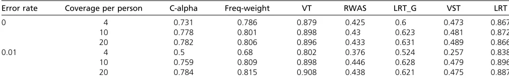
We evaluated the power of VST, LRT, and existing methods under two additional disease models. In the first disease model, causal variants must have MAF#1%, and have the same relative risk of 5 regardless of their MAF (ci = 0.2). This framework simulates a disease model where only rare variants are causal with the fixed effect size. The second disease model is similar to the PAR disease model discussed in Materials and Methods (PAR = 2%, ci = 0.1), but it includes additional protective variants. After choosingd del-eterious variants, we selected an additional 25% ofdvariants as protective to produce a ratio of 8:2 deleterious to pro-tective variants. Table 2 shows the power of methods in the
first disease model, and the VT method generally has the greatest power in this model. It is because VT assumes there exists an unknown MAF threshold such that variants whose MAF is less than the threshold are more likely to be involved in a disease, which is consistent with thefirst disease model. Note that the power of LRT is very close to that of VT in this disease model. In the disease model with protective var-iants, Table 3 shows that LRT is the most powerful method.
Applying VST and LRT to pooling of samples
We consider study designs in which a large number of pools are sequenced, where each pool includes the DNA of h/2 individuals and thus hhaplotypes. Typically, his relatively small (e.g.,h,20). This study design avoids the need for barcoding, and thus it further reduces the cost of the study. We compared the sensitivity of the proposed methods in scenarios with and without pooling of individuals’DNA sam-ples and also with and without considering sequencing error.
We generated simulation data using the scheme described above but in addition, simulated sequencing in pools. Wefirst generated haplotypes as described above, but then pooled case and control individuals separately into pools, with each pool containing the haplotypes ofh/2 individuals. Thus, each pool containshhaplotypes. Coverage is spread among these haplotypes. For example, in a pool containing DNA fromfive diploid individuals (i.e., 10 haplotypes), coverage ofg= 50 will yield50/10 = 5 reads of each base on each haplotype. In other words, in these data, the number of observations of a particular base on a particular haplotype is sampled from a binomial distribution withp¼1=ðh100;000Þand
g100,000 trials.
To obtain a realistic characterization of the parameters used in our simulations (i.e., error rate and pooling accu-racy), and to assess the implications on study design under budget constraints, we evaluated the characteristics of a real data set taken from a case–control study of non-Hodgkin lymphoma (L. Conde, I. Eskin, F. Hormozdiari, P. M. Bracci, E. Halperin, and C. Skibola, unpublished data). We se-quenced two pools, each containing a mixture of DNA from fvie case individuals for whom GWAS data were available (see Materials and Methodsfor details). We then measured the coverage, pooling accuracy and error rate (seeFile S1). Particularly, we found that the pooling was highly accurate in terms of the number of reads coming from each sample, that the average coverage was 44 per base, and that the sequencing error rate was0.235%. This is consistent with error rate reported in other sequencing studies (Minoche
et al.2011; Huffordet al.2012). We used these parameters to simulate a full study, as described below.
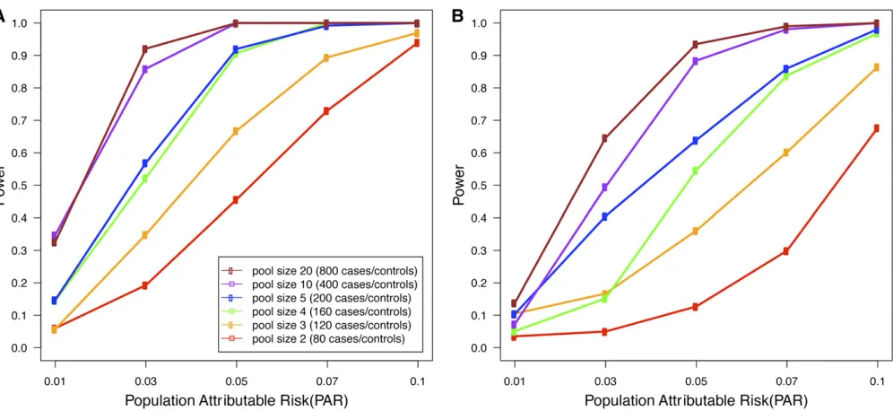
Pooling-based studies offer a trade-off between the introduction of uncertainty due to pooling and increased sample size. It is unclear what would be an optimal study design under a budget constraint. To explore this issue, we simulated a rare variants disease association study with realistic parameters, estimated from the study data. We assumed the budget allowed for 80 runs of the sequencing platform that produces reads at an average coverage of 44 per base per pool, with an error rate of 0.235%. We considered study designs involving an equal number of case and control pools. Figure 1 shows the expected power of LRT with various pool sizes for different values of PAR on two different data sets, where one data set has 20 SNVs in a region with ci = 50% while the other data set has 100 SNVs with ci = 10%. The results show that the power
increases dramatically as we increase the pool size from pool size 2 (80 cases and 80 controls) to pool size 20 (800 cases and 800 controls). This suggests that for a given budget, it is generally better to increase the number of individuals per pool as a means of increasing the sample size and that this outweighs the detrimental effects of pooling.
We note that the power of low-coverage sequencing studies is always at least as high as the power of a pooling study with the same number of samples and the same coverage per sample. The results demonstrated in Figure 1 also suggest that for a given budget, it is generally better to increase the number of individuals in the study and that this outweighs the detrimental effects of low-coverage sequencing.
LRT is robust to misspecified prior information
One of the drawbacks of the LRT statistic is that it uses prior probabilitiescifor a variant to be causal. Although one may use bioinformatics tools such as PolyPhen (Adzhubei et al.
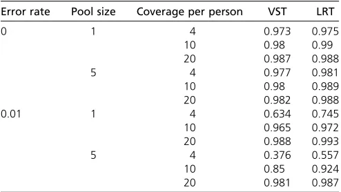
2010) or SIFT (Ng and Henikoff 2003) to estimate these priors, prior information may not always be accurate; there-fore it is important to assess the sensitivity of LRT to incor-rect prior information. To do so, we tested the LRT method with different prior information on the data that was gener-ated usingci= 0.1, as described inMaterials and Methods. Specifically, we provided the LRT method with priorsci= 0.02, ci = 0.5,ci= 0.5, and ci sampled from the uniform distributionU(0, 1). We used error ratee= 0.01, pool size of 5, and coverage of 20. The power of LRT with the correct prior information (ci= 0.1) is 0.987 (Table 4), while for the three tested scenarios, the power was 0.965, 0.968, and 0.943, respectively. The results demonstrate that even if prior information is incorrect, LRT still achieves high power,
Table 2 Power of different methods in a disease model in which only rare variants (MAF£1%) are causal with relative risk of 5 (ci= 0.2)
Error rate Coverage per person C-alpha Freq-weight VT RWAS LRT_G VST LRT
0 4 0.731 0.786 0.879 0.425 0.6 0.473 0.867
10 0.778 0.801 0.898 0.43 0.623 0.481 0.872
20 0.782 0.806 0.896 0.433 0.631 0.489 0.866
0.01 4 0.5 0.68 0.802 0.376 0.524 0.257 0.838
10 0.759 0.809 0.898 0.446 0.628 0.479 0.896
20 0.784 0.815 0.908 0.438 0.621 0.475 0.887
Tested methods were C-alpha (Nealeet al.2011), Freq-weight similar to the Madsen–Browning method (Madsen and Browning 2009), variable threshold (VT) (Priceet al.
2010), RWAS (Sulet al.2011b), LRT_G (Sulet al.2011a), and our proposed methods (VST and LRT).
Table 1 Power of different methods, on 1000 data sets and a region with 100 rare SNVs
Error rate Coverage per person C-alpha Freq-weight VT RWAS LRT_G VST LRT
0 4 0.062 0.659 0.872 0.668 0.817 0.973 0.975
10 0.062 0.713 0.903 0.688 0.854 0.98 0.99
20 0.067 0.722 0.903 0.692 0.858 0.987 0.988
0.01 4 0.051 0.174 0.208 0.269 0.286 0.634 0.745
10 0.066 0.479 0.674 0.610 0.71 0.965 0.972
20 0.067 0.686 0.887 0.690 0.848 0.988 0.993
albeit lower than the power achieved by VST (0.981 in this case).
VST and LRT control type I error rates
To measure type I error rates, we generated 10,000 random data setsfitting the null hypothesis with afixed read error rate of 1% and coverage of 4 per person. We measured the rate of spurious association detection at a confidence threshold of 0.05 with VST and LRT. The detection rate was in the range 0.0480–0.0513 for the two methods, showing that type I error is well controlled. Similar results were ob-served in the cases where pools of five samples each were analyzed. We also measured the error rates at a more strin-gent threshold of 0.001, using 100,000 random data sets with an error rate of 1% and coverage of 4. The type I error rates for LRT and VST were 0.00097 and 0.00088, respec-tively, and this indicates that VST and LRT control the type I error rates correctly at the stringent threshold.
Discussion
We proposed two new methods (VST and LRT) that identify associations of groups of rare variants. We show through simulations that our methods outperform previous methods under different disease models. Importantly, unlike previous methods that allow no errors in sequencing and require high-coverage sequencing of individual samples, our meth-ods can be applied to low-coverage sequencing with errors. We demonstrate through simulations that in the presence of high error rates and low coverage, the power improvement of both LRT and VST over previous methods is substantial. These simulations are based on a disease risk model where rarer variants have higher effect sizes, and we also explored additional disease risk models, often used in previous methods. When only rare variants are causal with the same effect size, the VT method has the greatest power because the assumptions of the VT statistic are consistent with the assumption of the disease model. However, LRT has comparable power to that of VT in this model. When the disease risk model contains protective variants, we show that LRT is the most powerful method. We note that VST can be easily modified to incorporate protective variants by taking the square of its statistic and that the modified VST achieves similar power to LRT when protective variants are present (data not shown).
In addition to the simulated data, we used a real data set from a study of non-Hodgkin lymphoma to obtain param-eters related to the sequencing technology and pooling strategy. We estimated coverage and error rates of sequenc-ing, and we verified that pooling can be performed ac-curately on a small number of samples (five in this case). Our proposed methods can also be applied to the scenario in which a large set of small pools is sequenced, and we used the estimates of the sequencing error rates to simulate the power of a pooled association study, when the number of samples per pool varies (from 1 to 20), but the number of pools is fixed. Based on our experiments, we believe that sequencing-based association studies should include as many individuals as possible by applying low-coverage sequencing and pooling when necessary.
Whereas LRT is generally more powerful than VST in most simulations, VST has several advantages over LRT. Importantly, VST makes fewer assumptions on the model; particularly it does not require prior information on the probability of a variant to be causal, and when incorrect prior information is specified, VST achieves higher power than LRT. VST is also a natural extension of several previous methods such as RWAS (Sul et al. 2011b), VT (Priceet al.
2010), and the Madsen–Browning test (Madsen and Browning 2009), which consider a weighted sum of differences in mutation counts; therefore, understanding the relation tween VST and LRT provides an insight on the relation be-tween LRT and previous methods. Additionally, VST is Table 3 Power of different methods in a disease model in which 20% of causal variants are protective
Error rate Coverage per person C-alpha Freq-weight VT RWAS LRT_G VST LRT
0 4 0.054 0.417 0.653 0.471 0.646 0.456 0.956
10 0.069 0.46 0.712 0.472 0.689 0.506 0.987
20 0.07 0.473 0.713 0.478 0.699 0.515 0.99
0.01 4 0.053 0.14 0.164 0.17 0.191 0.222 0.685
10 0.066 0.304 0.468 0.376 0.495 0.425 0.955
20 0.06 0.458 0.673 0.465 0.67 0.491 0.976
PAR was 0.02 withci= 0.1 Tested methods were C-alpha (Nealeet al.2011), Freq-weight similar to the Madsen–Browning method (Madsen and Browning 2009), variable threshold (VT) (Priceet al.2010), RWAS (Sulet al.2011b), LRT_G (Sulet al.2011a), and our proposed methods (VST and LRT).
Table 4 Power with pooling and errors, on 1000 data sets and a region with 100 rare SNVs
Error rate Pool size Coverage per person VST LRT
0 1 4 0.973 0.975
10 0.98 0.99
20 0.987 0.988
5 4 0.977 0.981
10 0.98 0.989
20 0.982 0.988
0.01 1 4 0.634 0.745
10 0.965 0.972
20 0.988 0.993
5 4 0.376 0.557
10 0.85 0.924
20 0.981 0.987
a simpler method than LRT, and it can be easily imple-mented and modified, allowing a moreflexible framework. Our methods directly utilize allele counts from sequenc-ing data to perform rare variants association testsequenc-ing, and an alternative approach is to call genotypes from allele counts and perform the testing. One may use a linkage disequilib-rium aware method for genotype calling (Duitama et al.
2011) or methods based on sophisticated models to improve the accuracy of calling. However, this approach has several drawbacks. First, it is considerably computationally inten-sive because aforementioned genotype calling methods gen-erally require extensive computation. Second, in low-pass sequencing, it is very difficult to call rare variants correctly because of an insufficient number of reads covering rare variants. Third, rare variants are not usually in linkage dis-equilibrium (LD) with other variants, and hence the LD aware method for genotype calling may not be very accurate for calling rare variants. Hence, power loss may be inevita-ble if methods attempt to call genotypes from low-pass se-quencing and perform rare variants association testing. In addition, we showed in our simulation that even when gen-otypes are called correctly in the high-coverage scenario, our methods are more powerful than other methods. This means that even if other methods are able to correctly infer geno-types from low-pass sequencing, our methods would be still more powerful.
Acknowledgments
E.H. is a faculty fellow of the Edmond J. Safra Bioinformatics Center at Tel-Aviv University. O.N. was supported by the Edmond J. Safra fellowship. E.H. and O.N. were also supported by the Israel Science Foundation, grant 04514831. J.H.S. and
E.E. are supported by National Science Foundation (NSF) grants 0513612, 0731455, 0729049, 0916676, and 1065276 and National Institutes of Health (NIH) grants K25-HL080079, U01-DA024417, P01-HL30568, and P01-HL28481. B.H. is supported by NIH–National Institute of Arthritis and Musculoskeletal and Skin Diseases grant 1R01AR062886-01. C.F.S., L.C., and J.R. are supported by NIH grants CA154643 and CA104682. P.B. is supported by NIH grants CA87014, CA45614, and CA89745. This research was also supported in part by the German-Israeli Foundation, grant 109433.2/ 2010 and in part by NSF grant III-1217615.
Literature Cited
Adzhubei, I. A., S. Schmidt, L. Peshkin, V. E. Ramensky, A. Gerasimova et al., 2010 A method and server for predicting damaging mis-sense mutations. Nat. Methods 7: 248–249.
Ahituv, N., N. Kavaslar, W. Schackwitz, A. Ustaszewska, J. Martin et al., 2007 Medical sequencing at the extremes of human body mass. Am. J. Hum. Genet. 80: 779–791.
Bar-Lev, S. K., and P. Enis, 1988 On the classical choice of vari-ance stabilizing transformations and an application for a Poisson variate. Biometrika 75: 803.
Bromiley, P. A., and N. A. Thacker, 2001 The effects of a square root transform on a Poisson distributed quantity. TINA Memo No. 2001–010. Available at http:www.tina-vision.net/docs/ memos.php.
Brown, K. M., S. Macgregor, G. W. Montgomery, D. W. Craig, Z. Z.
Zhao et al., 2008 Common sequence variants on 20q11.22
confer melanoma susceptibility. Nat. Genet. 40: 838–840. Cohen, J. C., R. S. Kiss, A. Pertsemlidis, Y. L. Marcel, R. McPherson
et al., 2004 Multiple rare alleles contribute to low plasma lev-els of hdl cholesterol. Science 305: 869–872.
Davison, A. C., and D. V. Hinkley, 1997 Bootstrap Methods and Their Application, Vol. 1. Cambridge University Press, Cambridge/ London/New York.
Decker, R., and D. Fitzgibbon, 1991 The normal and Poisson ap-proximations to the binomial: a closer look. Technical Report 82.3. Department of Mathematics, University of Hartford, Hart-ford, CT.
Duitama, J., J. Kennedy, S. Dinakar, Y. Hernández, Y. Wu et al., 2011 Linkage disequilibrium based genotype calling from low-coverage shotgun sequencing reads. BMC Bioinformatics 12 (Suppl 1): S53.
Easton, D. F., K. A. Pooley, A. M. Dunning, P. D. P. Pharoah, D. Thompsonet al., 2007 Genome-wide association study
identi-fies novel breast cancer susceptibility loci. Nature 447: 1087– 1093.
Erlich, Y., K. Chang, A. Gordon, R. Ronen, O. Navon et al., 2009 Dna sudoku–harnessing high-throughput sequencing for multiplexed specimen analysis. Genome Res. 19: 1243– 1253.
Eskin, E., 2008 Increasing power in association studies by using linkage disequilibrium structure and molecular function as prior information. Genome Res. 18: 653–660.
Gorlov, I. P., O. Y. Gorlova, S. R. Sunyaev, M. R. Spitz, and C. I. Amos, 2008 Shifting paradigm of association studies: value of rare single-nucleotide polymorphisms. Am. J. Hum. Genet. 82: 100–112.
Hanson, R. L., D. W. Craig, M. P. Millis, K. A. Yeatts, S. Kobeset al., 2007 Identification of pvt1 as a candidate gene for end-stage renal disease in type 2 diabetes using a pooling-based genome-wide single nucleotide polymorphism association study. Diabe-tes 56: 975–983.
Hufford, M. B., X. Xu, J. van Heerwaarden, T. Pyhäjärvi, J.-M. M. Chiaet al., 2012 Comparative population genomics of maize domestication and improvement. Nat. Genet. 44: 808–811. Kryukov, G. V., L. A. Pennacchio, and S. R. Sunyaev, 2007 Most
rare missense alleles are deleterious in humans: implications for complex disease and association studies. Am. J. Hum. Genet. 80: 727–739.
Li, B., and S. M. Leal, 2008 Methods for detecting associations with rare variants for common diseases: application to analysis of sequence data. Am. J. Hum. Genet. 83: 311–321.
Lin, D.-Y. Y., and Z.-Z. Z. Tang, 2011 A general framework for detecting disease associations with rare variants in sequencing studies. Am. J. Hum. Genet. 89: 354–367.
Madsen, B. E., and S. R. Browning, 2009 A groupwise association test for rare mutations using a weighted sum statistic. PLoS Genet. 5: e1000384.
Manolio, T. A., F. S. Collins, N. J. Cox, D. B. Goldstein, L. A. Hindorff et al., 2009 Finding the missing heritability of complex diseases. Nature 461: 747–753.
Minoche, A. E., J. C. Dohm, and H. Himmelbauer, 2011 Evaluation of genomic high-throughput sequencing data generated on Illu-mina hiseq and genome analyzer systems. Genome Biol. 12: R112. Neale, B. M., M. A. Rivas, B. F. Voight, D. Altshuler, B. Devlinet al., 2011 Testing for an unusual distribution of rare variants. PLoS Genet. 7: e1001322.
Neyman, J., and E. S. Pearson, 1933 On the problem of the most efficient tests of statistical hypotheses. Philos. Trans. R. Soc. Lond. A Contain. Pap. Math. Phys. Character 231: 289–337. Ng, P. C., and S. Henikoff, 2003 SIFT: predicting amino acid
changes that affect protein function. Nucleic Acids Res. 31: 3812–3814.
1000 Genomes Project Consortium, 2010 A map of human ge-nome variation from population-scale sequencing. Nature 467: 1061–1073.
Price, A. L., G. V. Kryukov, P. I. W. de Bakker, S. M. Purcell, J. Staples et al., 2010 Pooled association tests for rare variants in exon-resequencing studies. Am. J. Hum. Genet. 86: 832–838. Pritchard, J. K., 2001 Are rare variants responsible for suscepti-bility to complex diseases? Am. J. Hum. Genet. 69: 124–137. Pritchard, J. K., and N. J. Cox, 2002 The allelic architecture of
human disease genes: common disease-common variant. . .or not? Hum. Mol. Genet. 11: 2417–2423.
Schunkert, H., I. R. König, S. Kathiresan, M. P. Reilly, T. L. Assimes et al., 2011 Large-scale association analysis identifies 13 new susceptibility loci for coronary artery disease. Nat. Genet. 43: 333–338.
Skibola, C. F., P. M. Bracci, E. Halperin, L. Conde, D. W. Craiget al., 2009 Genetic variants at 6p21.33 are associated with suscep-tibility to follicular lymphoma. Nat. Genet. 41: 873–875. Sul, J. H., B. Han, and E. Eskin, 2011a Increasing power of
group-wise association test with likelihood ratio test, pp. 452–467 in Proceedings of the 15th Annual International Conference on Re-search in Computational Molecular Biology, RECOMB’11 edited by V. Bafna and C. Sahinalp. Springer-Verlag, Berlin/Heidelberg, Germany.
Sul, J. H., B. Han, D. He, and E. Eskin, 2011b An optimal weighted aggregated association test for identification of rare variants involved in common diseases. Genetics 188: 181–188. Wellcome Trust Case Control Consortium, 2007 Genome-wide association study of 14,000 cases of seven common diseases and 3,000 shared controls. Nature 447: 661–678.
GENETICS
Supporting Information http://www.genetics.org/lookup/suppl/doi:10.1534/genetics.113.150169/-/DC1
Rare Variant Association Testing Under
Low-Coverage Sequencing
Oron Navon, Jae Hoon Sul, Buhm Han, Lucia Conde, Paige M. Bracci, Jacques Riby, Christine F. Skibola, Eleazar Eskin, and Eran Halperin
FILE S1
MATERIALS AND METHODS
RELATIVE ABUNDANCE OF INDIVIDUALS’ DNA IN POOLS
The estimation of minor-allele frequency assumes knowledge of the relative abundance of each
individual’s DNA in each pool (implicitly or explicitly). It is therefore important to have a means of
estimating these relative abundances. To do this, we took advantage of the genotype data available
from the GWAS. In each pool, we selected SNVs that had a genotyping success rate of
100%
in the GWAS, which were unambiguously mapped to the genome (using the Varietas portal by
(P
AANANEN, C
ISZEKand W
ONG2010); the reference genome used was GRCh37) and that were
observed in at least 30 reads during sequencing. Furthermore, we required that no indels were
found at these sites during the alignment phase. 298,853 such SNVs were available for men, and
298,703 for women. At such SNVs, the proportion of major allele reads out of total reads is
expected to correspond to the number of major alleles carried by individuals in the pool, adjusted
for the individuals’ DNA’s relative abundance in the pool. We found the least-squares estimators
of the relative abundances in the following manner: in a pool with
h
k/
2
individuals and data for
m
SNVs, let
A
be the
m
×
h
k/
2
matrix corresponding to the minor allele counts times
1
/
2
, so that
A
ij= 0
,
0
.
5
or
1
if individual
j
carries 0, 1 or 2 copies of the minor allele of SNV
i
, respectively.
Let
x
be an
h
k/
2
×
1
column vector of relative abundances, so
x
i
equals the relative abundance
of individual
i
in the pool. Lastly, let
b
be the
m
×
1
column vector of the observed minor allele
frequencies in the pool, so that
b
iequal the proportion of minor alleles read out of total reads of
SNV
i
. The least-squares estimator of the relative abundances vector
x
is found by solving the
following optimization problem:
arg min
x
1
2
k
Ax
−
b
k
2 2
subject to
0
≤
x
i≤
1
, i
= 1
, . . . , h
k/
2
hk/2X
i=1
x
i= 1
(1)
Using the
lsqlin
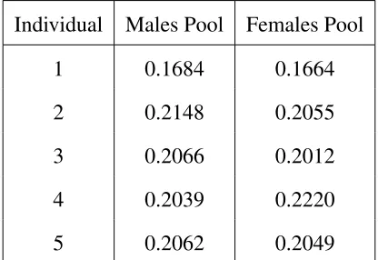
function in MATLAB, we found the least-squares estimators of relative
abun-dances listed in table 1. In both the men and women pools, relative abunabun-dances were generally
similar, though not exactly equal.
Individual
Males Pool
Females Pool
1
0.1684
0.1664
2
0.2148
0.2055
3
0.2066
0.2012
4
0.2039
0.2220
5
0.2062
0.2049
Table 1: Relative abundances in pools of individuals’ DNA.
ESTIMATION OF SEQUENCING ERROR RATE
To estimate the read error rate of the sequencing platform, we leveraged the GWAS data. We
selected a set of 18,163 SNVs in the pool of men (and 16222 in the pool of women) for which the
genotype minor allele counts are 0 for all five individuals in the GWAS, and which had at least
50 sequencing reads. We interrogated the proportion of minor alleles out of total alleles read at
each such position. For a SNV which was correctly genotyped, this proportion is approximately 0,
occasionally with small deviations produced by sequencing error. We discarded 88 SNVs in men
(68 in women) which had a proportion
>
0
.
05
, as we suspect they might represent genotyping
errors. At the remaining SNVs, 2489 of the 1084400 reads in men were minor allele (2203 out of
912938 in women). We thus estimated the sequencing error rate to be
0
.
229%
per base per read
in the men’s pool and
0
.
241%
in the women’s pool, assuming a simplistic error model in which
the rate of error is fixed across pools and independent of the position along the read and of the
nucleotide being read. It should be noted that in a more realistic error model of high-throughput
sequencing platforms, error rates do potentially depend on these factors.
ESTIMATION OF MINOR ALLELE FREQUENCY FROM SEQUENCING
DATA WITH ERRORS
The methods presented in this work rely on the estimated minor allele frequencies from
sequenc-ing data. To estimate these frequencies, we use a maximum likelihood approach with a
sim-ple error model. Note that more sophisticated models are possible, using error patterns
spe-cific to the sequencing platform, for example (e.g., (D
EP
RISTO, B
ANKS, P
OPLIN, G
ARIMELLA,
M
AGUIREet al.
2011; B
ANSAL2010; M
CK
ENNA, H
ANNA, B
ANKS, S
IVACHENKO, C
IBULSKISet al.
2010)). If necessary, such models can be readily substituted for the one presented in this
section.
Consider a set of
P
pools, each containing a mixture of DNA from several individuals (in
the case of low coverage sequencing without pooling, the size of each pool is
1
). Let
h
kdenote
the number of haplotypes in pool
k
(thus, pool
k
contains DNA from
h
k/
2
individuals), and let
α
idenote the relative abundance of individual
i
’s haplotypes in the pool, so that
P
hk/2i=1
α
i= 1
(the relative abundances are assumed to be known, and a method to estimate them is described
above). The pools undergo sequencing, generating observations of the minor and major alleles at
each genomic position. Our goal is to estimate
p
, the minor allele frequency across all pools, for
each genomic position.
Let
e
be the known (or estimated) error rate of the sequencing platform, and for pool
k
let
x
kbe the observed counts of the minor allele,
y
kthe observed counts of the major allele, and
z
k=
x
k+
y
k. For individual
i
in pool
k
, let
t
kibe the number of
i
’s chromosomes that carry the minor
allele, so that
t
ki∈ {
0
,
1
,
2
}. Finally, let
~t
kdenote the minor allele count vector
(
t
k1
, . . . , t
khk/2)
. To
estimate
p
, we observe that
t
ki∼
B
(2
, p
)
, and that
P r
(
~t
k|
p
) =
hk/2
Y
i=1
P r
(
t
ki|
p
) =
hk/2
Y
i=1
2
t
k ip
tki(1
−
p
)
2−tki(2)
Furthermore, when reading a single base from a pool
k
with the minor allele vector
~t
k, the chance
to observe a minor allele, denoted by
f
k(
~t
k)
is
f
k(
~t
k)
,
(1
−
e
)
hk/2
X
i=1
α
it
k i2
+
e
hk/2
X
i=1
α
i(2
−
t
ki
)
2
(3)
(to see this, note that we observe a minor allele if we either sample and read a minor allele
without
error
or sample and read a major allele
with error
). Therefore
x
k, the observed minor allele count
in pool
k
, follows a Binomial distribution:
x
k∼
B
(
z
k, f
k(
~t
k))
(4)
The likelihood of
p
for a particular pool
k
is then:
L
(
p
;
x
k, y
k) =
P r
(
x
k, y
k|
p
)
=
X
~tk∈{0,1,2}hk /2
P r
(
x
k|
z
k, ~t
k)
·
P r
(
~t
k|
p
)
=
X
~tk∈{0,1,2}hk /2
z
kx
k(
f
k(
~t
k))
xk(1
−
f
k(
~t
k))
zk−xk·
hk/2
Y
i=1
2
t
k ip
tki(1
−
p
)
2−tki(5)
And the full likelihood function is simply the product of the above across all
P
pools. Note that
we can write
a
k~tk,
zk
xk
(
f
k(
~t
k))
xk(1
−
f
k(
~t
k))
zk−xk, and then the likelihood function is
L
(
p
;
~
x, ~
y
) =
P
Y
k=1
X
~
tk∈{0,1,2}hk /2
a
~ktkhk/2
Y
i=1
2
t
k ip
tki(1
−
p
)
2−t ki
(6)
in which
a
~ktkdoes not depend on
p
, and can therefore be pre-calculated to speed up calculations.
We also denote
S
~tk,
hk/2
X
i=1
t
kiand
I
~tk,
hk/2
X
i=1
[
t
ki∈ {
2
,
0
}
]
(7)
(so that
I
~tkis the count of
t
ki’s which equal 2 or 0), and note that
hk/2
Y
i=1
2
t
kip
tki(1
−
p
)
2−tki= 2
I~tkp
S~tk(1
−
p
)
hk−S
~
tk
(8)
To find the value of
p
which maximizes
L
, we calculate the natural logarithm of the likelihood
function, and take its first derivative:
d
dp
lnL
(
p
;
~
x, ~
y
) =
P
X
k=1
P
~tk
a
~ktk2
I~tk
p
S~tk−1(1
−
p
)
hk−S~tk−1
(
S
~tk
−
h
k·
p
)
P
~tka
k~tk
2
I~tk