Improvements to the THOR Neutral Particle Transport Code on High-Performance Computing Systems via Acceleration, Parallelization, and Performance Analysis.

ABSTRACT

YESSAYAN, RAFFI ALEXANDER. Improvements to the THOR Neutral Particle Transport Code on High-Performance Computing Systems via Acceleration, Parallelization, and

Performance Analysis. (Under the direction of Dr. Yousry Y. Azmy).

As the availability and capability of high-performance computing (HPC) resources has

grown, so has the demand for high-fidelity simulations. Unfortunately, for methods like the

three-dimensional discrete ordinates approximation to the neutron transport equation, the cost

of high-fidelity simulations climbs rapidly because of the high dimensionality of the phase

space. Simulations can reach into the billions of degrees of freedom and require weeks to run

on unaccelerated, serial implementations of the method. For many applications, this run time

is intractable. To address this, modern codes must implement more advanced algorithms, such

as iterative acceleration and parallelism to reduce run times and better capitalize on computing

resources. When implemented efficiently and given sufficient resources, these methods can

reduce a two-week simulation to hours or minutes. However, these advanced methods may

also introduce complications. Depending on the implemented iterative method, acceleration

techniques, such as diffusion synthetic acceleration, can be resource heavy, while others, such

as Chebychev acceleration, can be unstable for certain problems. Parallelism introduces the

requirement for inter-process communication and, for certain methods, asynchronicity.

Modifications and analysis have been performed on the THOR neutral particle

transport code to implement the above improvements. THOR is intended to enable simulation

of complex geometries in a variety of scenarios, ranging from reactor simulation to

non-proliferation and, as such, must provide capabilities for a variety of applications. This work

describes four major efforts to improve THOR’s capabilities and bring it closer to production

level. First is the implementation of Chebychev power iteration acceleration, a low resource

cost method that reduces iteration count ~2x versus the existing fission source extrapolation and roughly comparable to some implementations of the high-memory usage JFNK solver.

This implementation also includes control logic designed to improve the stability of the method

for challenging problems. Second is the implementation of angular domain decomposition

mid-of ~10x to ~100x depending on available resources and problem parameters. The third item,

in pursuit of optimizing parallel performance, is the development of a modular parallel

performance model. This model captures the run time of THOR’s mono-energetic, zeroth

spatial order, unaccelerated inner/outer iteration solver to within ~5% for reasonably large

problems. The model is designed such that future modifications to the THOR code or to the

parameters of interest (e.g. adding group or spatial order dependence), can be easily added.

This makes the performance model a powerful tool not just for evaluating the efficiency of

existing code, but also for performing comparative studies and localizing inefficiencies in later

additions to THOR. A long-term goal of the THOR project is to enable massively parallel

spatial domain parallelism on 105+ processors. The implementation of the spatial domain

decomposition (SDD) algorithms on unstructured meshes is a massive undertaking beyond the

scope of this work. However, Task four lays the groundwork for this capability by analyzing

the communication inefficiencies present in PIDOTS, a three-dimensional Cartesian mesh

code which implements a parallel Gauss-Seidel SDD algorithm. This analysis demonstrates

that the high count, small-message communication paradigm used by PIDOTS leads to

communication slowdowns on the order of 10x for 105 processors and identifies steps that can

© Copyright 2018 Raffi Alexander Yessayan

Improvements to the THOR Neutral Particle Transport Code on High-Performance Computing Systems via Acceleration, Parallelization, and

Performance Analysis

by

Raffi Alexander Yessayan

A thesis submitted to the Graduate Faculty of North Carolina State University

in partial fulfillment of the requirements for the degree of

Master of Science

Nuclear Engineering

Raleigh, North Carolina

2018

APPROVED BY:

_______________________________ _______________________________

DEDICATION

To my Mom and Dad, Lynn and Arthur Yessayan, for a lifetime of unconditional love,

BIOGRAPHY

Raffi Alexander Yessayan was born in Charlotte, North Carolina on July 21st, 1993 to

Lynn and Arthur Yessayan. He lived in Charlotte until being accepted at North Carolina State

University in Raleigh, North Carolina. During his undergraduate career, he pursued significant

coursework in both nuclear engineering and computer science. Additionally, for two years, he

worked as a teaching assistant in both introductory computing and Fortran programming

courses. In 2015, he graduated Summa Cum Laude with a Bachelor of Science in nuclear

engineering, minors from both the French and Computer Science departments, and having

completed the University Honors Program.

For his graduate coursework, he remained in North Carolina State University’s

Department of Nuclear Engineering and began studying optimization and parallelization

techniques for unstructured mesh neutron transport codes under the direction of Dr. Yousry Y.

Azmy. He is a recipient of the Consortium for Nonproliferation Enabling Capabilities Graduate

ACKNOWLEDGMENTS

I would like to thank my advisor, Dr. Yousry Y. Azmy, for his support and guidance

throughout my graduate career. I would also like to thank Dr. Sebastian Schunert for

contributing his insight and experience to my project, especially with regards to the inner

workings of THOR. Finally, I would like to thank my parents for always providing support

and encouragement throughout my academic career.

The work of the author is based upon work supported by the Department of Energy

National Nuclear Security Administration under Award Number(s) DE-NA0002576.

This report was prepared as an account of work sponsored by an agency of the United

States Government. Neither the United States Government nor any agency thereof, nor any of

their employees, makes any warranty, express or implied, or assumes any legal liability or

responsibility for the accuracy, completeness, or usefulness of any information, apparatus,

product, or process disclosed, or represents that its use would not infringe privately owned

rights. Reference herein to any specific commercial product, process, or service by trade name,

trademark, manufacturer, or otherwise does not necessarily constitute or imply its

endorsement, recommendation, or favoring by the United States Government or any agency

thereof. The views and opinions of authors expressed herein do not necessarily state or reflect

TABLE OF CONTENTS

LIST OF TABLES ... viii

LIST OF FIGURES ... ix

1 Introduction ... 1

1.1 The Neutron Transport Equation... 1

1.2 Iterative Neutron Transport Solvers ... 4

1.3 The THOR Neutral Particle Transport Code ... 6

1.4 Desired Improvements ... 7

1.5 Selected Improvements ... 8

1.6 Thesis Outline ... 9

2 Iterative Acceleration Methods ... 10

2.1 Introduction ... 10

2.2 Literature Review ... 10

2.2.1 Fission Source Extrapolation ... 10

2.2.2 Coarse Mesh Rebalance ... 11

2.2.3 Diffusion Synthetic Acceleration ... 14

2.2.4 Chebychev Acceleration ... 15

2.3 Implementation... 16

2.4 Results ... 18

2.5 Future Work ... 22

3 Parallel Domain Decomposition ... 23

3.1 Introduction ... 23

3.2 Literature Review ... 23

3.2.1 Energy Domain Decomposition ... 23

3.2.2 Spatial Domain Decomposition ... 24

3.2.3 Angular Domain Decomposition ... 26

3.3 Implementation... 27

3.3.1 Work Splitting Routine ... 28

3.3.2 Parallel Execution ... 29

3.3.3 Communication ... 30

3.4.1 Scaling Studies ... 32

3.4.2 Synthetic Communication Modeling ... 36

3.5 Future Work ... 38

4 Parallel Performance Modeling ... 39

4.1 Introduction ... 39

4.2 Literature Review ... 39

4.2.1 Amdahl’s Law ... 39

4.2.2 PPMs for Transport Codes ... 41

4.3 An Overview of the Falcon HPC System... 42

4.3.1 Physical Layout of Falcon ... 43

4.3.2 Network Topology of Falcon ... 44

4.3.3 Other Falcon Notes ... 44

4.4 Complications Stemming from the THOR Cell Solver ... 45

4.5 Methodology ... 46

4.6 Results and Model Validation ... 50

4.6.1 Evaluating the Influence of Canonical Tetrahedron Subdivision ... 50

4.6.2 The Communication Model ... 53

4.6.3 The Parallel Sweep Model ... 56

4.6.4 Evaluating the Model ... 58

4.6.5 The Unified THOR Parallel Performance Model ... 62

4.6.6 Future Work ... 63

5 Parallel Communication Effects ... 65

5.1 Introduction ... 65

5.2 Literature Review ... 65

5.2.1 The PIDOTS Code ... 65

5.2.2 HPC Topology & Communication ... 67

5.3 Results ... 69

5.3.1 Recreating the PIDOTS Scaling Problem ... 69

5.3.2 Justification of Crossover in the Weak Scaling Trends ... 74

5.3.3 Exploring Communication Cost Growth on Falcon ... 75

5.3.4 Modeling the Impact of the Latency Distribution... 78

6 Software Management Improvements ... 84

6.1 Version Control ... 84

6.2 Modular Code Restructuring ... 85

6.3 Formal Testing ... 86

6.4 Documentation and Testing Coverage Metrics ... 87

6.5 Automated Build System ... 87

6.6 Summary ... 88

7 Conclusions ... 89

7.1 Summary ... 89

7.2 Final Comments ... 90

REFERENCES ... 91

APPENDICES ... 95

APPENDIX A – FALCON TOPOLOGY ... 96

LIST OF TABLES

Table 1: Comparison of THOR solver methods [4] ... 20

Table 2: Summary of Falcon Hardware Layout ... 43

Table 3: Simple Cube Test - Canonical Tet Variation [33] ... 51

Table 4: Godiva - Canonical Tet Variation [33] ... 52

Table 5: C5G7 - Canonical Tet Variation [33] ... 52

Table 6: Percent Error for Interpolation Cases, from [33] ... 58

Table 7: Actual vs. Model Results for Takeda-IV & Godiva Cases ... 61

LIST OF FIGURES

Figure 1: Flow diagram of iterative transport solution ... 5

Figure 2: Example of level-of-detail based structured/unstructured mesh, from [16] ... 13

Figure 3: Behavior of Chebychev Acceleration Factors ... 21

Figure 4: Example PGS-SDD Domain ... 25

Figure 5: ADD Parallel Inner Iteration Scheme ... 30

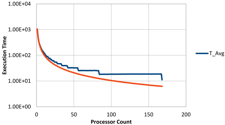
Figure 6: Comparison of Measured and Optimal Times for THOR ADD – Strong Scaling... 33

Figure 7: Strong Scaling for Angular Decomposition Problem plotting efficiency (%) versus the number of CPUs for S12 level-symmetric quadrature. [4] ... 34

Figure 8: Weak Scaling Results for 10k Tet Mesh with THOR ADD ... 35

Figure 9: Measured communication time for minimally loaded nodes performing AllReduce on Falcon. Data sets are labeled as [# of active processors per node] x [# of Nodes], from [4] ... 37

Figure 10: Measured communication time for partially loaded nodes performing AllReduce on Falcon. Data sets are labeled as [# of active processors per node] x [# of Nodes], from [4] ... 37

Figure 11: Possible Configurations for Canonical Tet Decomposition, from [32] ... 46

Figure 12: Hierarchical Timing Model Design, adapted from [33] ... 48

Figure 13: Updated representation of AllReduce Behavior on Falcon, adapted from [33] ... 50

Figure 14: Differing communication trends for p=288 and p=n(n+2) for S8, adapted from [33] ... 54

Figure 15: Differing communication trends for p=288 and p=n(n+2) for S12, adapted from [33] ... 55

Figure 16: THOR/HPC communication time fit, adapted from [33] ... 56

Figure 18: Linear relation between time and number of angles for a fixed value of p,

adapted from [33] ... 57

Figure 19: 400k tetrahedrons mesh model predictions vs measured, adapted from [33] ... 59

Figure 20: Evaluation of processor count dependence in grind time, adapted from [33] ... 60

Figure 21: Amended Model Cases, adapted from [33] ... 60

Figure 22: Final Model Predictions for Simple Cube, adapted from [33]... 63

Figure 23: Original PIDOTS Iteration Count as a Function of Processor Count; adapted from [22] ... 70

Figure 24: Original PIDOTS Weak Scaling Results adapted from [22] ... 71

Figure 25: PIDOTS Iteration Trends from FALCON ... 72

Figure 26: PIDOTS / Falcon Weak Scaling ... 72

Figure 27: Falcon PIDOTS Time Per Iteration ... 73

Figure 28: Histogram of 2-Hop Latency ... 77

Figure 29: Histogram of 3-Hop Latency ... 78

Figure 30: Sketch of Approximate PDF overlaid on Measured 2-Hop Data ... 79

Figure 31: Comparing Latency Models for p=64 ... 81

Figure 32: Comparing Latency Models for p=32,768 ... 81

Figure 33: Falcon IRU Structure and 1D Topology ... 96

Figure 34: Falcon 3D Topology ... 97

Figure 35: Falcon 4D Topology ... 97

Figure 36: Falcon 5D Topology ... 98

Figure 37: Falcon 6D Topology ... 98

Figure 38: Falcon Partial 7D Topology ... 99

Figure 39: PIDOTS / Fission Iteration Behavior ... 100

Figure 40: PIDOTS / Fission Total Execution Time ... 101

1

Introduction

1.1 The Neutron Transport Equation

The neutron transport equation describes the evolution of the neutron distribution over

a six-dimensional phase space formed by position, direction of motion, and energy. This

distribution is referred to as angular flux and, in this thesis, will be denoted as 𝜓(𝑟⃗, Ω̂, 𝐸, 𝑡),

where 𝑟⃗ is the position of the particle in cartesian (x,y,z) space within a volume 𝑑𝑟⃗, Ω̂ is the angular description of the particle’s direction of travel within a cone 𝑑Ω̂, E is the particle’s

energy within a band 𝑑𝐸, and t is the time of evaluation. A standard representation of this equation is given below [1]:

1 𝑣 𝜕 𝜕𝑡𝜓(𝑟⃗, Ω̂, 𝐸, 𝑡) + Ω̂ ∙ ∇⃗⃗⃗ 𝜓(𝑟⃗, Ω̂, 𝐸, 𝑡) + 𝜎𝑡(𝑟⃗, 𝐸)𝜓(𝑟⃗, Ω̂, 𝐸, 𝑡) = ∫ 𝑑𝐸′ ∞ 0 ∫ 𝑑Ω̂′ 4𝜋 𝜎_𝑠(𝑟⃗, Ω̂′_{→ Ω̂, 𝐸}′_{→ 𝐸)𝜓(𝑟⃗, Ω̂, 𝐸, 𝑡)} +𝜒(𝐸)

4𝜋𝑘 ∫ 𝑑𝐸

′ ∞ 0 ∫ 𝑑Ω̂′ 4𝜋 𝜈𝜎_𝑓(𝑟⃗, 𝐸)𝜓(𝑟⃗, Ω̂, 𝐸, 𝑡) +𝑞𝑒𝑥𝑡𝑒𝑟𝑛𝑎𝑙(𝑟⃗, Ω̂, 𝐸, 𝑡) (1)

In Eq. (1), 𝑣 represents the neutron speed, while 𝜎𝑡, 𝜎𝑠, 𝑎𝑛𝑑 𝜎𝑓represent, respectively,

the neutron cross sections for total interaction, scattering, and fission. The average number of

neutrons per fission event is given by 𝜈 and the resulting fission spectrum is given by 𝜒.

In this form, the first line of the equation represents the neutron sinks, in order: the

change in population with time, the out-streaming of particles, and interaction of particles. The

second line represents the scattering source, or the influx of particles into a volume of phase

space resulting from scattering interactions in other regions (𝑟⃗′, Ω_{̂, 𝐸′, 𝑡)}′ _{that deposit a particle}

into (𝑟⃗, Ω̂, 𝐸, 𝑡). The third line represents the contributions of fission events that result in a

of the original energy, 𝐸′ and that fission is assumed to be isotropic, i.e., it emits particles

evenly amongst the 4𝜋 directions of the unit sphere. The fourth line provides an arbitrary

external source of neutrons. The form given in (1) represents a combination of the two forms

represented in the THOR transport code, k-eigenvalue and fixed source. In THOR, for the former, k is part of the solution and can be any positive real value, while 𝑞𝑒𝑥𝑡𝑒𝑟𝑛𝑎𝑙 is taken to

be zero. For the latter, k must be less than 1 for a solution to exist and 𝑞_{𝑒𝑥𝑡𝑒𝑟𝑛𝑎𝑙} is a problem parameter.

While (1) provides a clean expression for the neutron transport equation, it is several

steps removed from a form convenient to implement into a numerical code. First, for the

purposes of this work, all problems will be taken to be steady state. As such, the time derivative

of the flux is zero and the corresponding term can be removed. Second, the continuous

variables in space, angle, and energy must be discretized, along with the integrals in angle and

energy. Multiple methods exist by which to perform this discretization. One method, which is

implemented by THOR, is the method of Discrete Ordinates [1], or the 𝑆_𝑛 method, which

divides the spatial volume into elements, the angles into a set of discrete ordinates, 𝑛 ∈ 1. . 𝑁,

and the energy range into a set of energy groups, 𝑔 ∈ 1. . 𝐺. The name 𝑆_𝑛 stems from the

subscript 𝑛 denoting the level of the angular quadrature used to approximate the angular

integrals.

Rewriting Eq. (1) in this form will require several stages. First, is the treatment of the

angular variable, Ω, via the method of Discrete Ordinates. In this method, the continuous

variable Ω is replaced with the finite set of directions, Ω𝑛, where 𝑛 = 1. . 𝑁. Via numerical

quadrature, this set of angles, paired with appropriate weights (𝑤_𝑛), can be used to replace

integrals over Ω with sums over 𝑤_𝑛Ω_𝑛. Finally, the scattering cross section, 𝜎_𝑠, which is a

function of both the incoming and outgoing angle, must be represented using an expansion in

spherical harmonics. Eq. (2) shows the Discrete Ordinates form of the transport equation with

Ω̂∇ψ_n(𝑟⃗, 𝐸) + 𝜎_𝑡ψ_n(𝑟⃗, 𝐸) = ∑ ∑ Υ_𝑙,𝑚(Ω̂_𝑛) ∫ 𝜎_𝑠(𝑟⃗, 𝐸′_{→ 𝐸)𝜙} 𝑙𝑚(𝑟⃗, 𝐸)𝑑𝐸 ∞ 0 𝑙 𝑚=−𝑙 𝐿 𝑙=0 +𝜒(𝐸)

4𝜋𝑘 ∫ 𝜈𝜎𝑓𝜙(𝑟⃗, 𝐸)

∞

0

𝑑𝐸 +𝑆𝑛(𝑟⃗, 𝐸)

4𝜋

(2)

Here, 𝜓_𝑛is the angular flux of the specific angle Ω_𝑛 and Υ_𝑙,𝑚 is the spherical harmonic

of degree 𝑙 and order 𝑚. All other variables subscripted with n are the same quantities as before, except now they only represent the component along direction n.

Next is the discretization of the energy domain. This will be done via the multigroup

method, which subdivides the energy range into a finite number of groups, G, and defines a set of G transport equations. This replaces integrals over energy with sums over each group. For quantities which are energy dependent, such as cross sections, the group average value is

defined as the flux weighted average over the energy range of the group. An example of the

multigroup discrete ordinates equations for continuous space is shown below [2].

Ω̂∇ψ_n,g(𝑟⃗) + 𝜎_𝑡,𝑔ψ_n,g(𝑟⃗) = ∑ ∑ ∑ Υ_𝑙,𝑚(Ω̂_𝑛)𝜎_𝑠𝑔′→𝑔(𝑟⃗)𝜙_𝑙,𝑔′𝑚 _(𝑟⃗) 𝐺 𝑔′=1 𝑙 𝑚=−𝑙 𝐿 𝑙=0 + 𝜒𝑔

4𝜋𝑘 ∑ 𝜈𝜎𝑓,𝑔′𝜙𝑔′(𝑟⃗)

𝐺

𝑔′=1

+𝑆𝑛,𝑔(𝑟⃗) 4𝜋

(3)

Here, 𝜓𝑔,𝑛is the angular flux of the specific group-angle combination. In this form, the

solution is only obtained along one ordinate, Ω̂𝑛, and one group, 𝑔, at a time.

The final phase dimension to discretize is space. There a variety of methods by which

to do this. However, in general, this step is performed by dividing the spatial domain into a set

of mesh cells. Each cell in the mesh has constant material properties and, as a result, constant

cross section. Next, a set of relations are defined to relate the cell center and outbound fluxes

As a result of this discretization, for a given angle, the flux in a cell is only dependent

on values local to that cell, sources and cross sections, and the flux incident on the cell from

its upstream neighbors. This allows for the use of a mesh sweep to evaluate the flux in all cells,

given a starting boundary with a known incident flux.

The known boundary, combined with the cell material information, can be used to solve

for the flux along a given ordinate in the cell and then propagate a cell-edge flux to the

downstream mesh neighbor. When this process is repeated across the entire mesh, it is referred

to as a sweep. After every angle has been swept, a new iterate of the flux profile in the domain

can be generated. As the next section will describe, this iteration process continues until a

sufficiently converged value of the flux solution is produced.

1.2 Iterative Neutron Transport Solvers

Moving from the mathematical expression of the numerical neutron transport equation

to a workable algorithm is relatively straightforward. Solution of the transport equation

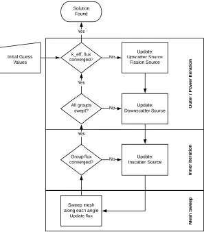
typically uses a set of two nested iterations: outer and inner. A flow diagram of these processes

is given in Figure 1. As it shows, the inner iteration is used to converge the in-scatter source,

while the outer iteration is used to converge the up-scatter source. By sweeping energy groups

Figure 1: Flow diagram of iterative transport solution.

Also of note is the lowest level of the iteration hierarchy, the mesh sweep. In this

operation, the current source and flux values are used to calculate a new flux iterate by moving

along each cell of the mesh, starting from a boundary with known in-flux. In this way, each

cell is solved using the known solution from its upstream neighbor. This sweep is performed

along the entire mesh for each discrete ordinate in the angular approximation. However,

individual sweeps are independent of one another until they are all completed. Once all sweeps

1.3 The THOR Neutral Particle Transport Code

The THOR neutral particle transport code is maintained at NCSU in collaboration with

Idaho National Laboratory (INL). It is a Fortran 95 application designed to solve the

three-dimensional discrete ordinates approximation discretized by unstructured tetrahedral meshes.

As a spatial approximation, it implements the arbitrarily high order transport method of the

characteristic type (AHOTC). The specifics of this implementation are beyond the scope of

this work and are detailed in [3].

To the best of author’s knowledge, THOR is unique in its implementation of this

arbitrarily high-order method on unstructured, tetrahedral meshes. As such, it provides a useful

testbed for the implementation and evaluation of modifications to the AHOTC method in

unstructured geometries. At the beginning of the author’s graduate program, THOR maintained

the following features:

• Serial solvers for both k-eigenvalue and external source problems using a traditional outer/inner iteration scheme

• Support for arbitrary energy groups, angular quadrature refinements, and spatial expansion order

• A Jacobian-Free Newton-Krylov Solver for k-eigenvalue problems

• Fission source extrapolation for acceleration of the outer iteration

Using these features, the THOR code could be used to evaluate a variety of scenarios

relevant to the modern nuclear engineering field. These include reactor core modeling [4],

source localization, and the evaluation of sub-critical weapons-grade material. However, the

neutron transport equation can be an extremely expensive problem to solve since it is

discretized in 6 variables – 3 directional, 2 angular, and 1 energy. Refinements to a given

problem can lead to massively increased computational costs. For small problems, this scaling

can yield several thousand degrees of freedom (DOF) and solving times on the order of

seconds. Even for many iterations of parameter studies, these costs are quite minor. However,

for larger problems, these costs can rapidly become intractable. For the largest problem run in

Lab (INL) [5], this scaling yielded approximately four billion DOF. This problem had a

solution time of ~2 weeks and was simply too time-intensive to run repeatedly. Unfortunately,

as evaluating a high-resolution reactor model, such as the ATR problem, forms a cornerstone

of the verification and validation plan for the THOR code, this posed an obvious challenge.

Based on the need to repeatedly and rapidly run problems on scales up to that of the ATR case,

it was determined that several modifications would need to be made to THOR.

1.4 Desired Improvements

As the ATR problem had demonstrated, the then-current implementation of THOR was

insufficient to tackle the massive problem sizes resulting from the desire for high-fidelity

results. Fortunately, there were a variety of possible modifications that could be made to THOR

to significantly speed up the solver.

However, there were also several limiting factors that restricted this field of choices.

Most important was the fact that previously completed work from another researcher had

verified the existing code via the method of manufactured solutions [6]. This meant that it was

desirable to introduce changes that encapsulated, rather than modified, existing pieces of code.

Maintaining this separation of functionality would allow for improvements to be made to the

code’s speed without risk of impacting verified code. The second constraint was related to the

future plans for THOR. Since many planned projects related to the capabilities of the

non-JFNK solvers, it would be ideal if the power iteration solver saw the greatest benefit from the

implemented changes.

From these needs and constraints, a goal could be developed – reduce the runtime of

the outer/inner iterative solvers as much as possible without significantly modifying existing

1.5 Selected Improvements

Based on the goal defined in section 1.4, there were two obvious paths for improving

the performance of THOR. First, implementation of a new acceleration scheme better than

fission source extrapolation and, second, the parallelization of one of the phase space

dimensions of the neutron transport equation.

For the first, a new acceleration method, there were again two options. In an outer/inner

solver schema, acceleration schemes can be applied to either (or both) the outer or inner

iterations. Several powerful inner iteration schemes exist which sharply decrease the required

number of inner iterations. Unfortunately, these are also typically more resource intensive,

requiring much more memory, and would require implementing significant modifications to

already-verified code. Additionally, k-eigenvalue problems in THOR are dominated by outer iterations. Some outer accelerations, such as the already implemented Fission Source

Extrapolation, are comparatively cheap and require only a short calculation at the end of an

outer iteration cycle. This small implementation and runtime overhead is balanced out by the

comparatively small acceleration they produce.

In the end, since eigenvalue problems are common for THOR, the lightweight,

non-intrusive nature of outer acceleration was found to be a better fit for the current needs. But,

given the expected performance of outer accelerations, it was also decided that simply

implementing a new outer acceleration would not provide a sufficient increase in performance.

To complement the outer acceleration some aspect of the code would also need to be

parallelized. From the variables involved in the transport equation, this left three options,

parallelism in space, angle, or energy.

Parallelism in energy is not ideal as the resulting algorithm is asynchronous due to

energy group coupling and, since the number of groups is typically small, limited in scalability.

While also asynchronous, spatial parallelism is a tempting option. The sheer number of

mesh cells in most problems allows for massive parallelization. Unfortunately, implementing

this parallel structure on unstructured meshes is a major undertaking and well beyond the scope

Finally, there is angular parallelism. Like spatial decomposition, the angular domain

grows in cost at an above-linear rate. However, unlike in the other options, angular

decomposition is synchronous. Angles are evaluated independently for most of the inner

iteration process. During the sweep, each angle is evaluated separately; and, at the end,

aggregate measures are generated form the completed result vector. Because of this, it would

be a relatively non-invasive task to implement an angular decomposition into a functioning

transport solver.

Based on this brief sampling of the available options for acceleration and

parallelization, an outer acceleration paired with angular parallelization best suits the needs of

the THOR project. The implementation and evaluation of the former will be detailed in Chapter

2, while the latter will be described in Chapter 3. Additionally, further evidence from literature

will be provided to justify each choice.

1.6 Thesis Outline

Each of the following chapters in this thesis will present work from single thrust area

of the THOR improvement project. For each thrust area, an overview of the existing literature

will be provided, followed by a discussion of the methodology, results, and conclusions related

to the work

Chapter 2 will discuss the development of the outer acceleration scheme decided on in

the previous sections. Chapter 3 will address the implementation of angular parallelization.

Next, Chapter 4 will present a compartmentalized method for parallel performance evaluation

of the THOR code. Chapter 5 will present an analysis of the performance of parallel codes on

a high-contention HPC system. Chapter 6 will highlight a variety of software management

improvements to the THOR project and explain their importance in the role of a

production-level neutronics code. Finally, Chapter 7 will provide conclusions and an overview of the net

2

Iterative Acceleration Methods

2.1 Introduction

As determined in sections 1.4 and 1.5, the optimal acceleration technique for this

project was not the one which demonstrated the largest increase in computational speed, but

rather the one which provided a reasonable amount of speedup for a relatively low cost in

implementation complexity and invasiveness. This section will review several common inner

and outer acceleration schemes. However, eigenvalue calculations are dominated by outer

iterations and several light-weight outer acceleration algorithms are readily available. In the

end, inner accelerations were deemed sub-optimal for our needs and work shifted focus to outer

acceleration methods. From this pool, Chebychev acceleration was selected. While there was

literature, [7], and anecdotal experience, [8], indicating that Chebychev was not an optimal

method, it was clearly documented in [9] and similar in implementation to the fission source

extrapolation already implemented in THOR. These benefits were deemed sufficient to

outweigh the negatives. In the end, with some modification to the standard algorithm,

Chebychev acceleration proved surprisingly effective and yielded speedups significantly better

than fission source extrapolation and roughly equal to some versions of the THOR JFNK

solver.

2.2 Literature Review

2.2.1 Fission Source Extrapolation

As described in [10], error-mode based fission source extrapolation (FSE) is one of the

most simplistic outer iteration acceleration schemes. However, this does not prevent it from

providing a useful degree of speedup in most problems. FSE is based on the fact that, as an

unaccelerated problem converges, the relative change in the fission density of the problem

be generated. Mathematically, this is achieved through the following steps. First, define the

iteration 𝑞 fission density error as the sum over all spatial cells:

𝑒𝑞 = ∑ |𝐷𝑞− 𝐷𝑞−1| (4)

where Dq is the fission density in iteration q. The fission density is calculated simply as the sum of all fissions in all groups.Next, this error term is used to evaluate an estimate of the eigenvalue and of the acceleration term as:

𝜆𝑞 = 𝑒

𝑞

𝑒𝑞−1 (5)

Θ𝑞 = 𝜆

𝑞

1 − 𝜆𝑞 (6)

This extrapolation term is then applied to both the scalar flux and the fission density:

𝐷𝑞′ _{= 𝐷}𝑞_{+ Θ}𝑞_(𝐷𝑞_{− 𝐷}𝑞−1_{) (7)}

𝜙𝑞′ = 𝜙𝑞+ Θ𝑞(𝜙𝑞− 𝜙𝑞−1) (8)

The authors of [10] mention that this approach is highly effective in converging k -eigenvalue problems and problems with significant up-scatter. However, under some cases, a

stable value of Θ will not be found and the acceleration scheme will not prove effective.

2.2.2 Coarse Mesh Rebalance

Coarse Mesh Rebalance (CMR), discussed in [11, 12, 13], is an inner acceleration

scheme that can be applied to the neutron transport equation. As the name implies, the method

involves superimposing a coarse mesh atop the existing fine mesh used by the transport solver.

The current cell-average flux iterate is then accelerated by generating a multiplicative term

Overall the methodology is rather simple. As described by [13] for the slab geometry

case, a set of balances are generated such that the flux in the coarse mesh satisfies:

𝜓

𝑛,𝑗+1₂

𝑙 ₌

{ 𝜓

𝑛,𝑗+1₂

𝑙−1₂

∗ 𝐹_𝑗𝑙, 𝜇_𝑛 > 0

𝜓

𝑛,𝑗+1₂

𝑙−1₂

∗ 𝐹_𝑗+1𝑙 ; 𝜇_𝑛 < 0

(9)

where the values for flux at the cell edges, 𝜓

𝑛,𝑗±1₂

∗ _,

are calculated using the balance relationship

implemented in the given code and the values of 𝐹_𝑗𝑙 are the acceleration coefficients. When

applied to all cells in the fine slab mesh, this forms a tridiagonal matrix which can be solved

to yield the 𝐹_𝑗𝑙 terms. Having determined a value for the acceleration term in each cell, an

accelerated iterate of the cell-center flux can be generated as:

𝜓_𝑛,𝑗𝑙 = 𝜓_𝑛,𝑗𝑙− 1

2_{∗ 𝐹}

𝑗𝑙 (10)

As the condition of two edges per cell in 1D yields a tri-diagonal matrix, it can be

inferred that higher dimensional problems will yield an increasingly wide block-diagonal

structure representing the edge coupling between cells.

While the CMR method has been a mainstay of simple, effective acceleration methods,

it presents several problems that make it unfit for our objectives described previously.

First, the presence of the matrix-solve means that CMR will have a significantly higher

per-iteration cost than non-matrix methods, both in memory and time utilization. While this is

not problematic for small problems, it will become a critical concern for extremely large

problems, which are both time and memory limited.

Further complicating the use of CMR concerns its application to unstructured meshes.

In the simple example described above, a fine slab mesh was coarsened into a less fine slab

mapping of the flux variables at cell edges. Applying this same routine to THOR would prove

challenging since an arbitrary group of tetrahedrons cannot be coarsened into another

tetrahedron. This difficulty could be avoided by using the same mesh for both the fine and

coarse meshes. Unfortunately, this approach makes the method inflexible as it would only

allow for that single configuration.

Several sources detail the process of overcoming the difficulties of unstructured-mesh

CMR [14, 15]. However, in both, the solution was to implement a degree of regularity to the

mesh. In doing so, the mesh was unstructured below some level of detail and structured above.

An example of this is provided from openMOC, [15], in Figure 2. Note that the implemented

acceleration is coarse-mesh finite difference, not CMR. Regardless, the system for handling

unstructured meshes is the same.

Figure 2: Example of level-of-detail based structured/unstructured mesh, from [16].

As can be seen on the left of Figure 2, even though the mesh is unstructured, it does

possess a degree of regularity stemming from the repetitive nature of the unit cell lattice. This

regularity is capitalized on to provide matching boundaries for CMR. Similarly, in [14], the

Unfortunately, due to the desired arbitrary-geometry nature of THOR, it would be

impossible to guarantee mesh repetitions of this sort in every problem without artificially

inserting them. As such, CMR is not a viable method for this application given its current

needs.

2.2.3 Diffusion Synthetic Acceleration

Alcouffe [7], describes a trio of Diffusion Synthetic Acceleration (DSA) methods for

use in multi-group, discrete-ordinates problems. The three treatments are designed to provide

a stable, highly-effective acceleration method. These stability improvements make DSA more

efficient than unaccelerated transport iterations under essentially all conditions except extreme

cases, such as unbounded heterogeneity [13]. This degree of improvement would provide a

massive boon to THOR.

DSA is characterized by the utilization of a neutron diffusion operator to accelerate the

inner iterations of the neutron transport solution. From a high-level viewpoint, the results of

an inner transport solve are used as the inputs to a diffusion-like solve. The diffusion solve

provides a greatly increased rate of convergence of the flux iterates. A significant benefit of

this method is that it is effective under most conditions, including those where true diffusion

would not be [7].

However, like CMR, the solution of DSA acceleration requires the creation of an

additional matrix system of equations in the iterative correction terms, consuming both

additional memory and execution time per iteration. However, given the results demonstrated

in [7], this increase in per-iteration cost would be easily outweighed by gains in iteration count

reduction. The comparison in [7] shows DSA consuming anywhere from ~3 to ~10 times fewer

iterations than unaccelerated transport. Additionally, the method proves similarly effective

when compared to Chebychev and CMR.

These substantial speedups, coupled with the evidence of guaranteed convergence

provided by [7]would seem to indicate that DSA is the optimal acceleration to implement into

multi-dimensional problems as material heterogeneity becomes unbounded.Furthermore, as [7] and

[18] discuss, DSA is most easily applied to fixed source problems. Applying it to general

eigenvalue problems can prove challenging. Since THOR primarily evaluates eigenvalue

problems, this weakness, coupled with the desire to modify verified code structures as little as

possible, rendered DSA suboptimal to implement for this project. There is still a significant

desire to implement it in the future as project needs and constraints evolve. But, for now, it is

not the optimal choice.

2.2.4 Chebychev Acceleration

From a review of the literature, Chebychev acceleration seems to be often used, but

rarely described. It is mentioned as an option or used for efficiency comparisons by [7], [9],

and [11], but the implementation is only fully described in Hébert’s work, [9]. Like fission

source acceleration, Chebychev acceleration does not require a matrix evaluation [11]. Instead,

it uses an estimate of the dominance ratio to modify the next flux iterate using a superposition

of old iterates. This makes it extremely cheap to implement in terms of run time costs since it

only involves a set of uncoupled expressions.

In the method described in [9], Chebychev acceleration is implemented as a cyclical

process. First, a series of unaccelerated iterations are used to loosely converge the dominance

ratio. Then, some fixed number of accelerated iterations are performed, with each one using

the dominance ratio estimate as an acceleration parameter. After the fixed number of

accelerations is complete, relations based on the Chebyshev polynomials are used to extract

the equivalent un-accelerated dominance ratio. This new dominance ratio is used to drive a

new cycle of accelerated iterations. At each step in the process, the Chebychev relationships

are used to generate two terms, 𝛼 and 𝛽, which are combined with the old iterative flux

estimates to provide an improved new flux estimate.

In the same publication, Hébert compares the Chebychev method to a proposed

than Chebychev acceleration to implement but yields only marginally better results in terms of

iteration count.

Similarly, in [7], Chebychev is used as one of a variety of acceleration methods for

benchmarking. Of note from these other methods are the unaccelerated, Coarse Mesh

Rebalance, and Diffusion Synthetic Acceleration results. As would be expected from the

earlier discussion, the DSA inner acceleration scheme requires far fewer iterations and is more

stable than any other method. However, it has the most complicated implementation and

highest per-iteration computational cost. Of the remaining methods, Chebychev is generally

able to converge faster than both CMR and unaccelerated inner iterations. However, there is

one case each [7] where Chebychev fails to outperform the other methods. These failures are

attributed to insufficient convergence in the initial guess value for the dominance ratio. Both

[11] and [9] emphasize that the method may become unstable if the initial dominance ratio

guess is poor.

2.3 Implementation

The Chebychev acceleration method implemented in THOR follows closely the form

developed in [9]. A summary of this method, along with the modifications made to it in our

implementation is presented here.

First, a set of unaccelerated iterations is performed while estimating the dominance

ratio as the 2-norm of the flux difference in iteration 𝑘 and 𝑘 − 1:

𝜎𝑘+1= |𝜙𝑘− 𝜙𝑘−1|₂ (11)

When the dominance ratio estimate k+1 _{exceeds 0.5, a Chebychev acceleration cycle} is triggered and the current iteration, 𝑘, is designated 𝑛∗. In this cycle, m Chebychev

acceleration steps are executed. During each of these steps denoted with an iterative index p, a

𝜙𝑛∗+𝑝+1 = 𝜙𝑛∗+𝑝+ 𝛼(𝜙𝑛∗+𝑝− 𝜙𝑛∗+𝑝−1) + 𝛽 ∗ (𝜙𝑛∗+𝑝−1− 𝜙𝑛∗+𝑝−2)

𝑝 = 1, . . , 𝑚

(12)

𝛼 =

{

2

2 − 𝜎𝑛∗₊₁ 𝑝 = 1

4 𝜎𝑛∗₊₁∗ (

cosh[(𝑝 − 1)]

cosh(𝑝𝛾) ) 𝑝 > 1

(13)

𝛽 = {

0 𝑝 = 1

(1 −𝜎

𝑛∗₊₁

2 ) −

1

𝛼(𝑝) 𝑝 > 1

(14)

𝛾 = cosh−1₍ 2

𝜎𝑛∗₊₁− 1) (15)

The acceleration defined above can be applied for m iterations. After this, the acceleration cycle ends and an update to the dominance ratio must be performed to allow for

the re-initiation of the Chebychev scheme. The process of reconstructing the unaccelerated

dominance ratio at the conclusion of a Chebychev cycle is as follows:

𝐸 =||(𝜙

𝑛∗+𝑚_{− 𝜙}𝑛∗+𝑚−1_)|

2|

|(𝜙𝑛∗₊₁

− 𝜙𝑛∗

)|₂

(16)

𝐸∗ _{= [𝐶}

𝑚−1∙

(2 − 𝜎𝑛∗+1₎

𝜎𝑛∗₊₁ ]

−1

(17)

𝐶𝑚−1(𝑥) = cosh [(𝑚 − 1) ∗ cosh−1(𝑥)]

The two factors, 𝐸 and 𝐸∗, represent the achieved and theoretical error reduction for a

Chebychev cycle of m steps. Next, they are combined to provide an estimate of the unaccelerated dominance ratio via:

𝜎𝑛∗+𝑚+1₌ 𝜎

𝑛∗+1

2 ∙ [cosh (

𝑐𝑜𝑠ℎ−1(_𝐸𝐸∗)

Assuming the accelerated iteration has remained stable, the new dominance ratio can

be used immediately as the 𝜎𝑛∗+1 value of a new Chebychev cycle of length m.

Unfortunately, this method was found to be frequently unstable for a variety of test

cases. As a result, several modifications were made to the algorithm proposed by [9] outlined

above and the modified version was implemented in THOR.

The most significant of these modifications was to recalculate the theoretical error

reduction, 𝐸∗, during every iteration, replacing the value of m with the current value of p. Using

this continuous update of the 𝐸∗,(𝑝−1), the effectiveness of the Chebychev cycle can be

determined.

If, after a user-determined number of cycles, the achieved error reduction is less than

the 𝑝 − 1 theoretical error reduction, the cycle is deemed ineffective and aborted. From

evaluation of the code performance, ineffective cycles seemed to occur when initial dominance

ratio estimate was poorly converged. As such, when a cycle is aborted a configurable number

of power iterations are queued up prior to the start of the next Chebychev cycle. By doing this,

the acceleration benefits of Chebychev can be maintained while at the same time actively

monitoring for poor convergence.

In addition to this algorithmic change, general stability was improved by tightening the

criteria under which Chebychev iterations start. This was accomplished by requiring a small

number of power iterations to be performed after the initial 𝜎 > 0.5 condition is reached. This

delays the onset of the Chebychev system, but also tends to decrease the number of aborted

cycles.

2.4 Results

The original results from the implementation of this acceleration scheme were

presented in [4]. For that evaluation, the performance of the newly implemented Chebychev

method was compared to the existing unaccelerated, fission-source accelerated, and JFNK

solvers. To evaluate the effectiveness of the methods, a high-dominance ratio benchmark

homogenous cube with a side-length of 200cm and material properties: 𝜎_𝑡 = 1, 𝜎_𝑠 =

0.7, 𝜈𝜎_𝑓 = 0.39 𝑐𝑚−1. A one-dimensional version on this configuration is described in [19].

On this test domain, a monoenergetic flux was converged to 10−7 in scalar flux and 10−8 in

eigenvalue.

For comparison purposes, the default implementations of the THOR unaccelerated and

fission source accelerated solvers, see [6], were used. These simply implement the

methodologies described previously with no special modifications.

Additionally, 3 varieties of the THOR JFNK solver routine were exercised. These three

methods were JFNK-1 (2), JFNK-1 (4), and JFNK-2. The first two evaluate the nonlinear

function using a single outer and either 2 or 4 inner iterations. These limitations on the number

of iterations are designed to minimize the memory footprint of JFNK so that it can be applied

to larger problems without becoming memory constrained.

JFNK-2 abandons this memory constraint and allows for the construction of up to a

30-dimension Krylov subspace. Unfortunately, this method is extremely memory intensive, with

each dimension of the subspace requiring an additional copy of the angular flux moments for

the entire domain to be stored. This is obviously an intractable method for large problems, but

it can be used to provide significant speedup on otherwise challenging problems with small

domains.

As shown in Table 1, the implemented Chebychev acceleration performed quite well

compared to the non-JFNK transport solvers and performed reasonably well when compared

to the JFNK solvers with limited memory footprints. Note that, as is typical for THOR, two

inner iterations were performed per outer iteration for each of the three power iteration based

Table 1: Comparison of THOR solver methods [4].

Method Power/Newton Iteration count (Krylov It. Count)

Transport Sweep

Count Speedup

Power Iteration 2714 5428 1

Fission source

extrapolation 1109 2218 2.5

Chebychev

acceleration 667 1334 4.1

JFNK-1 (2) 8 (679) 1376 3.9

JFNK-1 (4) 7 (522) 2120 2.6

JFNK-2 7 (649) 657 8.3

From these promising speedup results, Chebychev acceleration fulfills the objectives

set forth for acceleration of THOR’s outer iterations. It provides a significant speedup in

general problems and does not incur significant calculation or storage overhead. The method

provides significant improvement over fission source extrapolation while maintaining a

comparable per-iteration computational cost and only requires the storage of an additional

scalar flux vector (as well as assorted scalars). Additionally, the method provides a roughly

equivalent speedup, lower-memory alternative to the JFNK-1 (2/4) methods. This serves a dual

benefit. First, it allows for larger problems to be solved, and second, it allows for transport

iterations to be observed directly by developers for debugging. By its nature, the JFNK solver

is comparatively minimalist in terms of in-process output compared to the more fully-featured

iterative solver output.

Unfortunately, Chebychev acceleration does not provide a perfect approach. As has

been noted several times in this chapter, the method is more prone to instability than the

unaccelerated and fission source solvers.

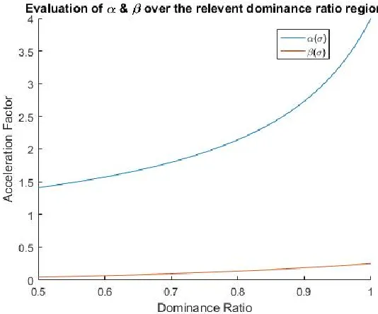
This instability stems from the inability of the Chebychev relations to provide

diminishing flux iterates. This is shown in the plot of 𝛼 and 𝛽 as a function of dominance ratio

in Figure 3. Since there is no point in the region where Chebychev acceleration is allowed that

provides negative acceleration factors, the method will always increase the flux. This will

eventually lead to instability in the solution if a value higher than that in the limit solution is

Figure 3: Behavior of Chebychev Acceleration Factors.

This acceleration behavior was the motivating factor behind the addition of the logic to

detect “ineffective” cycles. When the system begins to overshoot, the error climbs rapidly. As

such, when an increase in error is detected, the code stops the Chebychev iterations and uses

power iterations in an attempt to correct the divergence. While not completely effective, this

modification allowed the Chebychev routine to remain stable in several test cases where the

original algorithm [9] otherwise failed. The tradeoff in iteration count is unfortunate, but

worthwhile to increase the odds of convergence.

This instability precludes Chebychev acceleration from being used as a general

first-choice algorithm. However, it does allow it to be used to accelerate problems with known

solutions for scenarios such as benchmarks or to perform parameter studies on a problem for

which it is determined to be stable. This ability to rapidly re-run test cases is critical to

maintaining the ability to implement and debug new THOR features related to the evaluation

2.5 Future Work

It is likely that the Chebychev routines will remain unchanged for the near-term. The

currently implemented version fulfills the needs of ongoing research and performs sufficiently

well. But, as time allows, or as needs change, there are several improvements that could be

made to the algorithm. From discussions with [8], it appears that the stability and performance

of the Chebychev acceleration method can be dramatically improved through the addition of

further pre- and in-acceleration metrics. These metrics can be used to evaluate the readiness of

the problem for (further) acceleration and drive modified unaccelerated iterations to better

prepare the problem for Chebychev acceleration cycles.

Additionally, based on the discussion presented in the literature review, it would be a

significant improvement to THOR’s performance if DSA were implemented. This is a desired

3

Parallel Domain Decomposition

3.1 Introduction

At the beginning of this project, THOR was a serial code. Given the availability of

computing systems from moderate (10s to 100s of processors) to massive (105+ processors) in

the contemporary scientific computing environment, it seemed obvious that THOR could

benefit greatly from at least some degree of parallelism. As discussed in Chapter 1, the desired

features of the acceleration precluded energy and spatial domain decomposition. As such,

Angular Domain Decomposition (ADD) was pursued. Given that THOR’s typical problems

utilize angular quadratures of order S2 through S16, ADD is useful on the medium granularity parallel scale. This is ideal for its current stage of development as it keeps the code flexible

enough to run on personal workstations as well as on mid-scale HPC systems.

3.2 Literature Review

3.2.1 Energy Domain Decomposition

As described by [20], energy domain decomposition (EDD) faces two distinct

problems. The first is one of scaling and the second one of synchronicity.

Firstly, of the three parallelizable variables in a neutron transport problem, the number

of energy groups tends to be one of, if not the, smallest. This severely limits the degree of

parallelism that can be achieved. For a typical THOR problem, EDD would be limited to ~10

processors or, in the extreme case a few tens of groups. This lack of distributable work means

that the maximum speed-up from the method is inherently limited simply due to the low

number of processors which could be used.

While the first issue could be overcome if a given problem demanded many energy

groups, the issue of asynchronicity is more difficult to overlook. As discussed by [20] and

involved in the operation, the more iterations that are needed. This creates a situation in which

the per-iteration gains are penalized by losses in total iteration count.

EDD works by decomposing the loop over all energy groups, i.e., assigning each group

to different processors, just above the inner iteration level in Figure 1. This allows the

calculation for each energy group to proceed in parallel with each processor calculating an

in-scatter source and performing a one-group, all-angles sweep. Unfortunately, as the in-in-scatter

source is typically composed of both up-scatter and down-scatter components, this means that

no energy group will be operating with fully updated scattering source values. Thus, further

iterations will need to be performed to converge the in-scatter sources between the various

groups.

While this method would be possible to implement into THOR within the constraints

laid out in Chapter 1, EDD was deemed sub-optimal for implementation. Given the desire to

preserve the existing solver characteristics, a synchronous method is preferred. Additionally,

while EDD could offer a moderate speedup, concerns were raised about the limited scalability

of the method since THOR is typically used on few-group problems.

3.2.2 Spatial Domain Decomposition

Moving to the other end of the spectrum in scalability is spatial domain decomposition

(SDD). In this decomposition, the spatial mesh is decomposed and spread between several

processors. Now, rather than being responsible for a portion of the transport iteration, each

processor is responsible for an entire transport sweep/solve on a reduced domain. The solutions

from the partial domains are communicated and iterated over to produce a converged solution

for the entire domain.

A variety of SDD methods exist. However, since this topic will be revisited in Chapter

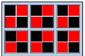
5, focus will be given to the parallel Gauss-Seidel method in [22]. In this method, the problem

domain is subdivided into a set of processor domains, where each processor domain contains

some number of red-black striped sub regions. An example of this is shown in Figure 4.

are converged by repeatedly sweeping over the red sub-domains, updating the boundary fluxes,

sweeping over the black cells, updating the boundary fluxes, and then performing a global

domain convergence check using the most current values for all cells.

Figure 4: Example PGS-SDD Domain.

Unfortunately, due to the need to propagate data between subdomains, this method is

also asynchronous. However, as the size of the spatial mesh is typically very large, thousands

to millions of cells, this decomposition provides significant opportunity for parallelization. The

results shown in [22] indicate scaling well into the tens of thousands of processors.

As mentioned, alternatives to the above PGS method exist. One class of these focuses

on parallelizing the sweep operation by identifying data dependencies between cells and then

parallelizing operations over cells with no unresolved dependencies. One of the earliest

examples of this is the Koch-Baker Alcouffe (KBA) algorithm, which identifies a number of

parallel task pipelines for a sweep and then assigns a processor to one of each of the resulting

sets of mesh cells [23]. Significant work has been conducted to further improve this style of

spatial parallelism, with research focusing on identifying optimal scheduling algorithms [24],

[25], [26]. These algorithms attempt to identify the most parallel configuration of mesh-angle

pair sweeping orders. By allowing multiple starting points and mesh-angle pairs

simultaneously, efficiency far greater than that of KBA can be achieved. Unfortunately, much

of this work is developed for Cartesian meshes, which have inherently known and

far more complicated and even include cycles. This makes the development of an optimal

scheduler for unstructured meshes a daunting task.

Much like DSA was suited for acceleration, SDD seems ideal for parallelization.

Unfortunately, there are several drawbacks that rendered it unsuitable for our purposes.

Foremost amongst these is the sheer man-hour cost of implementation. SDD has been

repeatedly demonstrated for structured meshes. However, it remains a relatively novel

approach on fully unstructured meshes. Implementation of SDD in THOR would form the

basis of a major project, likely larger in scope than the one detailed in this thesis.

3.2.3 Angular Domain Decomposition

Having eliminated EDD and SDD, the remaining variable-domain to decompose is

angle. In angular domain decomposition (ADD), the mesh sweep is decomposed such that N

mesh sweeps occur simultaneously, where N is the number of discrete ordinates in the quadrature set that correspond to explicit boundary conditions.

As [20]discusses, ADD provides a medium level of granularity. It is neither as coarse

as EDD nor as fine as SDD, but instead provides for several 10s to 100s of discrete workflows.

As shown from results in the GONT code,even an optimally implemented version of ADD is

capped at providing significant speedup in the range of 100s of processors [20]. Beyond this

point, the serial costs of the iteration begin to dominate and significantly decreasing speedups

are observed. Based on this fact, it is not reasonable to expect any implementation of ADD to

demonstrate the same scalability as SDD. However, since it is synchronous and more scalable

than EDD, it should generally perform better than that method.

ADD’s synchronicity stems from the fact that, during the sweep process, each angle of

the angular flux matrix is independent from all others. This is true only in Cartesian geometry

(no redistribution term) and when at least one boundary condition per dimension is explicit. It

is not until the generation of the spatial distribution of the angular moments of the flux that

Once all angular sweeps have been completed, the ADD algorithm can use an all-reduce operation to combine and redistribute the partial results from each ordinate [20]. This

provides a much simpler, and typically maximally compact, method for distributing the data.

Compared to SDD, where a processor only needs data from its adjacent neighbors, the

communication structure required by ADD is direct and typically requires no further logic than

that present in standard communication libraries.

Methods do exist to further optimize the communication behavior of the ADD method

[27]; however, as that work showed, the cost of communication typically is low enough that

effort is better spent improving non-communication performance. Additionally, given the

variety of HPC architectures and network interconnects that exist, it is unlikely that any

specific modification will provide a general improvement on all systems.

Regardless of these concerns, ADD provides a perfect match to the needs outlined in

Chapter 1. It provides a minimally invasive method for significant speedup on the scale of the

HPC computer available to the author. Furthermore, since the decomposition is synchronous,

it can be considered independently of the existing, verified, code. If the serial and parallel

versions return the same result, then the code is unaffected.

3.3 Implementation

Implementation of angular domain decomposition into THOR was a relatively

straightforward process, requiring none of the special handling that was seen with Chebychev

acceleration. The implementation consists of three parts: the work splitting routine, the parallel

section, and the communication phase.

Since the intended system for testing THOR is the Falcon HPC at INL, it was important

that the ADD algorithm be designed for message passing systems, not shared memory

architectures. Based on this need, the most straightforward path towards implementation was

to utilize the Open MPI [28], library. In doing so, each execution of the program now allows

components of the code. However, when a parallel section is reached, the work is divided

amongst processors as described in the next section.

3.3.1 Work Splitting Routine

In THOR, due to its use of the level-symmetric quadrature set, the number of angles in

a problem is given by

𝑁 = 𝑛(𝑛 + 2) (19)

Where the 𝑛 is the same quadrature order as given by the 𝑆𝑛 in the definition of the discrete

ordinates method. This means that in an order-𝑛 problem, there are 𝑁 parallel tasks. Again,

this is only true for 3D problems with explicit boundary conditions. To enable fair division of

this workload, the optimal number of tasks per processor is calculated at startup based on the

number of provided processors via:

𝑁_{𝑂𝑝𝑡𝑖𝑚𝑎𝑙} = ⌈𝑁

𝑝⌉ (20)

For executions where the number of processors, 𝑝, is a factor of the number of angles,

it is a straightforward matter to assign 𝑁_{𝑂𝑝𝑡𝑖𝑚𝑎𝑙} tasks to each processor. This provides an even

distribution of work and leads to the minimum amount of wasted CPU time during the parallel

portion. However, when the number of angles is not an integer multiple of the number of

processors, work must be assigned such that there is only a one task difference between the

most loaded and least loaded processor.

These needs are met by explicitly mapping a set of 𝑁_{𝑂𝑝𝑡𝑖𝑚𝑎𝑙} angles to each processor.

A more flexible approach to this mapping would be to simply allow each processor to pull an

ordinate from a queue as it completed its previous one. However, it was judged that this method

burdensome additional control logic. Because of this explicit mapping, a consistently slow

processor will continue to negatively impact the solve speed throughout the entire sweep rather

than allowing other processors to pick up its slack. However, since the expected use of this

capability is the 𝑁 = 𝑝 scenario, this effect is negligible.

3.3.2 Parallel Execution

The implementation of a parallel code on a message-passing architecture can be

considered as a set of 𝑝 independent programs that only interact via communication. As such,

technically, all aspects of the THOR code now exist in parallel. This means that for each of the

𝑝 instances, a full copy of all program data is available in local memory. However, the 𝑝

independent programs may have different values for their variables.

Using the index assigned to each processor and the work splitting routine defined

previously, the ADD implementation of THOR can algorithmically select the set of angles to

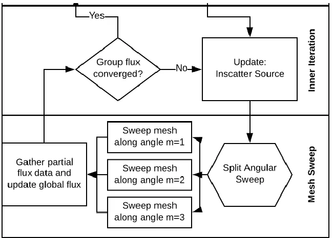
be swept by a given processor. Returning to the flow diagram given in Figure 1, the modified

ADD flow diagram is shown in Figure 5. For compactness, the outer iteration portion has been

omitted as it remains unchanged.

Given the use of a message-passing paradigm, there exist 𝑝 processes executing at all

stages of the routine, including the serial portions. However, except for the three-way split

after the “Split Angular Sweep” stage, all 𝑝 processors are performing identical calculations.

Once the code reaches the split, the work is divided amongst the available processors (a

3-processor solve is shown in Figure 5). Based on this explanation, the work in the serial section

is performed 𝑝 times, but by 𝑝 processors. This means that execution time of the serial portion

remains invariant to changes in 𝑝. Contrasting this is the parallel section, where a total of 𝑁

tasks are split amongst 𝑝 actors. This means that the expected execution time of the parallel

section should decrease as 1

𝑝. The control flow also reflects the fact that this method is

synchronous. From the point where work is assigned, to the point where flux is accumulated,

Figure 5: ADD Parallel Inner Iteration Scheme.

3.3.3 Communication

The remaining aspect of the parallel scheme is the recombination of the partial-sum of

the angular fluxes. For the discrete ordinates method implemented in THOR, only the flux

angular moments need to be retained between iterations. This allows for significant memory

savings and provides a unique benefit during ADD communication. During the angular

sweeps, rather than maintaining a large vector of angular fluxes, the data can be compacted

into the typically much smaller number of angular moments necessary to compute the

scattering source in the inner iterations. This is done on the fly by accumulating contributions

from each computed angular flux in each cell as it is calculated into the angular moments for

that cell. As such the accumulated flux angular moments for group 𝑔 in cell 𝑖 can be given as

𝜙_𝑔,𝑖𝑙𝑚 =1

8∑ 𝑤𝑛𝑌𝑙𝑚

𝑒 _(Ω̂

𝑛) ∗ 𝜓𝑔,𝑖(Ω̂𝑛) 𝑁

𝑛=1