Improvement of the seismic fragility analysis by use of the methods of structural reliability and safety analysis

20th International Conference on Structural Mechanics in Reactor Technology (SMiRT 20) Espoo, Finland, August 9-14, 2009 SMiRT 20-Division 7, Paper 1655

Improvement of the Seismic Fragility Analysis by Use of the Methods of

Structural Reliability and Safety Analysis

Dietrich Klein

, Fritz-Otto Henkel

a

Woelfel Beratende Ingenieure GmbH + Co. KG, 97204 Hoechberg, Germany, e-mail: [email protected]

b

Woelfel Beratende Ingenieure GmbH + Co. KG, 97204 Hoechberg, Germany, e-mail: [email protected]

Keywords: Fragility analysis, scaling method, structural reliability and safety analysis,

1

ABSTRACT

The commonly used method for calculation of seismic fragilities is the scaling method. This method uses lognormal mathematics for the calculation of the conditional probability of failure. It is known, however, that the use of lognormal mathematics may be an erroneous approach in the tails of the lognormal distributions. To overcome this shortcut an improvement of the method based on themethod of structural reliability and safety analysis as it is used for reliability analysis of civil structures is proposed. The application of the improved method is demonstrated by an illustrative example.

2

INTRODUCTION

The key task in a seismic probabilistic safety analysis (PSA) is the fragility analysis. Seismic fragility of a structure or equipment item is defined as the conditional probability of its failure at a given value of the seismic input response parameter. The peak ground acceleration (PGA) is commonly used as input response parameter. The objective of fragility evaluation is to estimate the ground motion capacity of the item and its uncertainty. Because there are many variables in the estimation of this ground acceleration capacity, the fragility is described by a family of fragility curves to reflect the uncertainty in the fragility estimation.

The mostly used method for fragility analysis is the scaling method. In this method the family of fragility curves is described by three parameters: the median ground acceleration capacity , and the logarithmic standard deviations R for randomness and U for uncertainty. The fragility parameters , R

and U are estimated by an intermediate random variable, the factor of safety F, which relates the

acceleration capacity A to the earthquake level specified for design ASSE. The factor of safety is the product

of individual factors which describe the conservatism in the design. All factors of safety are assumed to be log normally distributed, principally for its calculation convenience.

3

SCALING METHOD

From the numerous publications about the scaling method only the papers of Kennedy et al (1980) and Kennedy and Ravindra (1984) may be referenced here. In the report of Reed and Kennedy (1994) the basic methodology is described and detailed example fragility calculations are given. The basic content of this method is summarized as follows.

The fragility for a component corresponding to a particular failure mode is expressed in terms of the best estimate of the median ground acceleration capacity and two random variables εR and εU. The ground

acceleration capacity, A, is then given by:

A = ·εR·εU (1)

The random variables R and U are assumed to be log normally distributed with unit medians and

logarithmic standard deviations R and U respectively. The variable R represents the inherent randomness

about the median. It cannot be reduced by more detailed evaluation, or by gathering more data. The variable

U represents the uncertainty in the median value due to lack of understanding of the physical properties,

errors in calculated responses due to use of approximate modelling of the structure, usage of engineering judgment and others. With perfect knowledge U would be zero.

The frequency of failure at any non-exceedance probability level Q can be derived as:

! " # $

% &

' ( ) '

+

(

= *

R 1

U (Q)

) A / A ln( )

A ( P

(

(2)

where ( …) is the standard Gaussian cumulative distribution function.

The median ground acceleration capacity is related to the earthquake level specified for design ASSE

by a factor of safety F(:

= F(·ASSE (3)

For equipment in structures the factor of safety is the product of 4 individual factors which are again the product of further factors:

F = FS·F ·FRE·FRS (4)

where FS = strength factor; represents the ratio of ultimate strength (or strength at loss of function)

to the stress calculated for ASSE. It is composed by the inherent safety factor regarded in

the design calculations and the randomness of the material strength.

F = inelastic energy absorption factor; accounts for the fact that an earthquake represents a limited energy source and many structures or equipment are capable of absorbing substantial amounts of energy beyond yield without loss of function.

FRE = equipment response factor; recognizes that in the design-analyses, the equipment

response was computed using specific (often conservative) deterministic response parameters for the equipment.

FRS = structure response factor; describes the response characteristics of the structure at the

location

4

STRUCTURAL RELIABILITY AND SAFETY ANALYSIS

4.1 General Methodology

The calculation of the failure probability is accomplished in three steps:

1. Mechanical Model: definition of the failure modes (limit state functions) for each element of the structure or component as functions of deterministic parameters a0 and stochastic parameters Xj

Gi ( a0; X1; X2; X3 ··· Xn ) = 0 (5)

2. Stochastic Model: definition of the stochastic parameters of the basic variables Xj (e. g. probability

density function, mean or median value, variance or standard deviation). The randomness of the basic variables is split into the inherent randomness and model uncertainty. The modal uncertainty may also be regarded by additional basic variables.

3. Probability Analysis: calculation of the probability of exceedance of the limit state functions

pfi = Pi { Gi ( a0; X1; X2; X3 ··· Xn ) < 0 } (6)

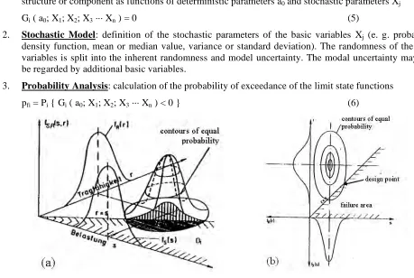
Figure 1. Failure probability, graphical representation

Fig. 1 shows a graphical representation of the fundamental case with two basic variables S for the load and R for the resistance and a linear failure limit state function G = R – S = 0.The two-dimensional joint probability density function fS,R is plotted as a hump in the s-r-space. The volume of the hump within the

unsafe region corresponds to the probability of failure. This presentation allows for a generalisation to multiple basic variables an arbitrary distribution density functions and any, also non-linear limit state functions The failure probability pf is the multi-dimensional integral of the joint density function fX1,X2,···Xn

over the failure area G(x1, x2, ··· xn). If, and only if, the basic variables Xi are statistically independent, the

joint density function fX1,X2,···Xn is equal to the product of the individual density functions fX1·fX2···fXn.

!

!!

= x,x ,...x 1 2 n 1 2 n

) x ,... x , x ( G

f ... f (x ,x ,...x ) dx dx ...dx p

n 2 1 n 2 1

(7)

Different solution strategies were developed to solve the reliability integral. The mostly used methods are simulations (e. g. Monte-Carlo simulation with importance sampling) and approximation methods based on the second moment-first order procedures. Computer codes for the calculation of failure probabilities which are based on the above mentioned methods are available. In the presented investigations the part COMREL of the reliability program STRUREL (2003) is used.

4.2 Application for improvement of the scaling method

The outlined methodology is used to improve the shortcuts in the scaling method. The major improvement is the appropriate definition of the failure mode as analytical formulation of the limit state function. This formulation allows the definition of other than lognormal distributions and the consideration of correlations between the stochastic parameters.

Failure occurs if the over all safety factor F is less than 1. By insertion of the different safety factors as defined in eqn (4) the limit state function reads:

(

)

F F A / A S S S F G RS RE SSE SSE oper lim = ! ! " " !

# _µ (8)

where Slim = limit strength, e. g. stress

Soper = stress under operation loads

SSSE = stress under design earthquake (e. g. safe shutdown earthquake)

ASSE = design earthquake level

Fµ , FRE , FRS see under eqn (4)

Slim, Soper , SSSE , FRE , FRS and F are the basic variables. They may be functions of other stochastic

parameters with different properties. The dispersions of the basic variables are separated in a part for the inherent randomness and a part for uncertainty as in the scaling method. The deterministic parameter A/ASSE

is introduced to allow for a parameter study with A as variable parameter.

The probability of exceedance of the limit state function is calculated with respect to the parameter A for the peak ground acceleration. In the first step the uncertainty in the median is investigated. The fragility is analyzed with the uncertainty parameters U alone and the ground acceleration capacity A as well as the

values of the basic variables Xi is read for selected probabilities of exceedance, e. g. at 95%, 50% and 5%.

These values are the respective median values of the random parameters at the selected confidence limits. In the second step the fragilities are calculated for each set of the selected median values of the basic variables with the inherent randomness R alone. The result is the median (50%) as well as the upper (5%) and lower

(95%) confidence fragility curves. The HCLPF value for the acceleration is read from the 95% confidence fragility curve at the probability of failure of 0,05.

For further use the calculated fragility curves are approximated by lognormal functions with the HCLPF value as reference value. The median value A50% is the acceleration at the probability of failure of 0,5 in the

50% confidence curve. The logarithmic standard deviations for uncertainty und randomness are:

!! " # $$ % & ' = ( % 95 % 50 U A A ln 65 . 1 1 !! " # $$ % & ' = ( HCLPF % 95 R A A ln 65 . 1 1 (9)

where A50% = acceleration at the probability of failure of 0,5 in the 50% confidence curve

A95% = acceleration at the probability of failure of 0,5 in the 95% confidence curve

AHCLPF = acceleration at the probability of failure of 0,05 in the 95% confidence curve

5

ILLUSTRATIVE EXAMPLE

5.1 Description

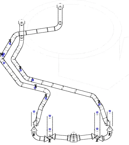
Figure 2. Isometric view of selected pipe run

This example allows for the exemplary investigation of the typical parts of a pipe line, like active components (valves), passive components (pipeline and tank) and the major types of supports (friction bearings, spring hangers and shock absorbers). Following failure modes are investigated:

• integrity of the pipe line: • functionality of the valves:

• functionality and stability of the supports: • integrity and stability of the rapid shutdown tank

The response of the complete pipe line was analysed with a detailed finite element model. The earthquake responses were calculated by use of the response spectrum modal analysis (RSMA) with floor response spectra as input. The floor response spectra were calculated with a simplified stick model of the reactor building by use of the time history modal analysis (THMA). The soil stiffness was calculated by a comprehensive analysis of the soil-structure interaction in the frequency range.

5.2 Application of the scaling method

The application of the standard scaling method is demonstrated here for the flow stress failure of the pipe. The mostly stressed section is the pipe bend between the valves. The fragility parameters are listed in Table 1. The strength factor FS is calculated by comparison of the limit stress with the equivalent stress according

KTA 3211.2 after superposition of operation loads and earthquake loads. The inelastic energy absorption factor is a function of the ductility ratio µ according eqn (10) with ε as additional random variable which reflect the error in eqn (10).

F = #" 2µ!1 (10)

The equipment response factor FRE is again a product of factors influencing the response variability. The

parameters are identified in Table 1. The structure response factor FRS is also a product of factors similar to

Fmed !R !U

Strength factor FS 5,68 0,07 0,26

Inel. energy absorption factor Fµ 2,24 0,16 0,16

Qualification method factor FQM 1,00 0,00 0,00

Spectral shape factor FSA 1,20 0,20 0,20 ASSE = 2,10 m/s 2

Modelling factor FM 1,00 0,00 0,15 A50% = 62,4 m/s 2

Damping factor FD 1,10 0,04 0,20 A95% = 21,2 m/s 2

Mode combination factor FMC 1,00 0,15 0,00 A5% = 183,5 m/s 2

Earthquake comp. comb. factor FEC 1,00 0,14 0,14 HCLPF = 11,0 m/s 2

Equipment response factor FRE 1,32 0,29 0,35

Structure response factor FRS 1,77 0,21 0,46

Total equipment factor Ftot 29,73 0,40 0,65

5.3 Application of the proposed improvement

By insertion of eqn (10) into eqn (7) the limit state function reads

(

)

F F

A / A S S

S S 1 2 G

RS RE

SSE SSE

H , oper p , oper

lim =

! ! " "

" ! "

µ

! #

$ (11)

where Soper,p = normal operation stresses from internal pressure

Soper,H = normal operation stresses from dead load and temperature

The stochastic parameters are listed in table 2. The ductility is defined as shifted lognormal distribution to account for the fact, that cannot be less than 1. The equipment response factor FRE and

structure response factor FRS are defined here as used in the scaling method, Table 1. This simplification is

appropriate because FRE and FRS as products of other lognormal parameters are again log normally

distributed. The normal operation stress from internal pressure is approached as deterministic parameter Soper,p = 44,3 N/mm

2

. As design earthquake level the peak ground acceleration ASSE = 2,1 m/s 2

is used.

Table 2. Stochastic parameters of basic variables

Stochastic parameters distrib. dim. median

type value randomn. uncert.

Strength Slim LN N/mm2 325,00 0,06 0,20

Operating loads Soper,H LN N/mm

2

8,14 0,00 0,18

Earthquake loads SSSE LN N/mm

2

48,01 0,00 0,10

Ductility ratio µ shift. LN -- 3,00 0,13 0,00

Ductility factor ! LN -- 1,00 0,00 0,16

Equipment response factor FRE LN -- 1,32 0,29 0,35

Structure response factor FRS LN -- 1,77 0,21 0,46

log. stand. deviation

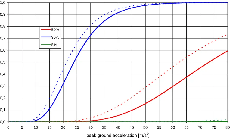
Fig. 3 shows the fragility curves with dashed lines for the results of the standard scaling method and bolt lines for the results of the improved method. In the presented case the standard scaling method is a good approximation on the safe side. This is because the dominating parameters are the equipment response factor FRE and structure response factor FRS, as can be seen by means of the sensitivities in Fig. 4. These two factors

comply with the preconditions for the application of the scaling method: log normal distribution of the parameters and multiplicative implementation in the limit state function.

Figure 3. Fragility curves: stress failure of pipe (dashed lines: scaling method, bold lines: improved method)

Figure 4. Sensitivities of basic variables: stress failure of pipe

The fragility parameters of the investigated failure modes are compared in Table 3. It is shown, that the

0,0 0,1 0,2 0,3 0,4 0,5 0,6 0,7 0,8 0,9 1,0

0 5 10 15 20 25 30 35 40 45 50 55 60 65 70 75 80

peak ground acceleration [m/s2]

50%

95%

5%

Table 3. Comparison of the fragility parameters

standard scaling method improved scaling method A50%

[m/s2]

random.

βR

uncert.

βU

HCLPF [m/s2]

A50%

[m/s2]

random.

βR

uncert.

βU

HCLPF [m/s2]

integrity of pipe line 62,4 0,40 0,65 11,0 73,2 0,38 0,68 12,8

functionality of valve 46,0 0,36 0,61 9,3 45,5 0,37 0,62 8,8

function of friction bearing 23,8 0,37 0,58 4,9 23,0 0,41 0,60 4,3

strength of spring hanger 30,3 0,36 0,58 6,5 29,7 0,38 0,59 6,0

strength of shock absorber 40,9 0,37 0,59 8,4 40,4 0,39 0,60 8,0

stability of tank 26,1 0,3 0,58 6,2 24,6 0,28 0,57 6,1

6

CONCLUSION

It is shown, that the method of the structural reliability and safety analysis, as it is used for reliability analysis of civil structures, can be applied to improve the standard scaling method with reasonable effort. This is demonstrated by a pipe run of the rapid shutdown system of a boiling water rector. For the investigated example the standard scaling method gives reasonable results compared with the improved method.

REFERENCES

Kennedy, R.P. et al. 1980. Probabilistic Seismic Safety Study of an Existing Nuclear Power Plant. Nuclear Engineering and Design, 59, pp 315-338.

Kennedy, R.P., Ravindra, M.K. 1984. Seismic Fragility for Nuclear Power Plant Risk Studies. Nuclear Engineering and Design, 79, pp 47-68.

Reed, J.W., Kennedy, R.P. 1994. Methodology for Developing Seismic Fragilities. Electric Power Research Institut (EPRI), TR-103959 Research Project, Final Report.