IEEE 802.11g,n Multi-Network Jamming Attacks - A Cognitive Radio Based Approach.

(1)

ABSTRACT

PRASAD, SUDARSHAN. IEEE 802.11g,n Multi-Network Jamming Attacks - A Cognitive Radio Based Approach. (Under the direction of Dr. David Thuente.)

Wireless networks are susceptible to jamming attacks, which can severely reduce the

network throughput. In our research, we study the behavior and the performance of

802.11g and 802.11n networks under hybrid jamming attacks of configuring a cognitive radio as a jammer. With characteristics such as fast channel switching, quick response

time and software reconfigurability, cognitive radios can be used not only to improve the

spectrum sharing management, but also to act as an effective jammer. We use OPNET

v16.0 and v16.1 to present various scenarios with cognitive radio based jamming attack

and its effect on throughput.

We use a single cognitive radio to simultaneously jam three networks in an energy

efficient manner and also to deny any channel change protocol by the targeted network

to avoid jamming. With respect to 802.11g, we attack the g band OFDM channels in

2.4 Ghz band directly using the fast channel switching capability of the cognitive radio. The jammer sequentially senses traffic on each of the networks without being part of

any network. We show how the cognitive radio can dynamically adjust its attack to the

traffic on each network. We evaluate the performance of three networks individually and

together under intelligent and reactive jamming.

In this research, we also consider three 802.11n networks and show how cognitive

radio based jamming attacks could be deployed at 5 GHz band. The cognitive radio uses

its dynamic power adaptibility feature to adjust its transmission power depending on the

jammer’s baseband frequency. We show how the cognitive radio jammer can be used to

(2)

IEEE 802.11g,n Multi-Network Jamming Attacks - A Cognitive Radio Based Approach

by

Sudarshan Prasad

A thesis submitted to the Graduate Faculty of North Carolina State University

in partial fulfillment of the requirements for the Degree of

Master of Science

Computer Science

Raleigh, North Carolina

2012

APPROVED BY:

Dr. Khaled Harfoush Dr. Mihail Sichitiu

(3)

DEDICATION

(4)

BIOGRAPHY

Sudarshan Prasad was born in Coimbatore, India. He graduated from Anna University

in 2006 with Bachelors degree in Computer Science (First class distinction). After his

graduation, he joined Sasken Communications Technologies Ltd in Chennai, India. With three years (2006 to 2009) of experience in performance optimizations and

mobile platforms and with zeal to purse Masters in Computer Science, he joined North

Carolina State University in fall 2009. While working towards his degree, he worked as a

Graduate Technical Intern for Mobile Wireless Group in Intel Corporation for 9 months

(5)

ACKNOWLEDGEMENTS

I would like to thank my advisor Dr. David Thuente. His guidance has really helped

me throughout my research. His willingness to help me with patience and interest has

motivated me all along my Masters program. I am thankful for all his time, ideas, and contributions provided in this research. It was really a wonderful and a stimulating

experience to have him as an advisor. I admire his depth of knowledge and his personal

qualities and I am grateful for the opportunity to work with him.

I am thankful and honored to have both Dr. Khaled Harfoush and Dr. Mihail Sichitiu

in my thesis committee.

I am grateful to my wonderful parents Dr. G.K. Prasad and Anusuya Prasad, who

have always motivated and encouraged me. Their love and affection has been a moral

support for me. My younger brother Anirudh, has also been of a great support. I would

like to thank my friends for all the help and advice they have provided me. My friends Krishna and Vivek have been a great source of knowledge and support. We had a very

good experience during our semesters along with lots of fun. Their help and support

would always be remembered. Thank you guys!

Vikram, Narayanan, Dinesh and Sethu have also helped me various ways. I would

also like to thank Sagar and Mithun for their valuable inputs and help provided during

(6)

LIST OF TABLES

Table 2.1 MAC layer parameters of 802.11g . . . 9 Table 2.2 Comparision of operational modes . . . 12 Table 2.3 MAC layer parameters of 802.11n . . . 16

Table 4.1 Timings of transmitting a 1500 byte packet in pure ’g’ network . . 32 Table 4.2 Average throughput at different data rates . . . 40 Table 4.3 Jamming Efficiency - Varying packet sizes with interarrival time of

exp(0.02) seconds . . . 41

(9)

LIST OF FIGURES

Figure 2.1 The basic CSMA/CA in 802.11b/g networks . . . 8

Figure 2.2 CTS-to-Self protection mechanism . . . 11

Figure 2.3 802.11n Channel Bonding . . . 14

Figure 4.1 Base scenario model with jammer . . . 27

Figure 4.2 Channel allocation for three networks . . . 27

Figure 4.3 OPNET node model for wireless workstation . . . 28

Figure 4.4 Attributes of wireless workstation . . . 28

Figure 4.5 Traffic generation parameters of a wireless workstation . . . 29

Figure 4.6 Baseline throughput total for three networks with no jamming . . 30

Figure 4.7 Attributes of jammer . . . 30

Figure 4.8 Constant and exponential periodic jamming . . . 34

Figure 4.9 Instantaneous - exponential jamming at 18 Mbps with 10 iterations. Each color represents one of the 10 iterations with different random seeds. . . 35

Figure 4.10 Average - exponential jamming at 18 Mbps with 10 iterations. Each color represents one of the 10 iterations with different random seeds. 36 Figure 4.11 Confidence Interval 95% : - instantaneous throughput for exponen-tial jamming at 18 Mbps with 10 iterations. Each color represents one of the 10 iterations with different random seeds. Black line represents the confidence intervals. . . 36

Figure 4.12 Confidence Interval 95% : - average throughput for exponential jamming at 18 Mbps with 10 iterations. Each color represents one of the 10 iterations with different random seeds. Black line represents the confidence intervals. . . 37

Figure 4.13 Exponential jamming at different data rates . . . 37

Figure 4.14 Exponential Jamming - Varying offered packet sizes (constant, total offered load) . . . 38

Figure 4.15 Exponential Jamming - Varying packet sizes (constant arrival rate) 39 Figure 4.16 Reactive Jamming - Three networks with different loads . . . 42

Figure 5.1 Single 802.11n network . . . 45

Figure 5.2 802.11n node attributes . . . 46

Figure 5.3 802.11n high throughput parameters . . . 46

Figure 5.4 Baseline average throughput of single 802.11n network without jammer . . . 47

Figure 5.5 Jammer attributes . . . 48

(10)

Figure 5.7 Jammer attacking edge of two adjacent OFDM channels . . . 50

Figure 5.8 Average Throughput - Jammer attacking edge of a 5 GHz channel with 20µW . . . 51

Figure 5.9 Base scenario with 3 networks in a single cell . . . 52

Figure 5.10 Jamming attacks in channels 36, 40 and 44 with 10 µW . . . 54

Figure 5.11 Jamming attack in channel 36 with 100 µW . . . 55

Figure 5.12 Average throughput - Periodic exponential jamming attack . . . . 56

Figure 5.13 Average Throughput - Exponential jamming attack at edges of adjacent channels . . . 57

Figure 5.14 Average Throughput - Exponential jamming attack at edges of adjacent channels with higher power . . . 57

Figure 5.15 Average Throughput - Exponential jamming attack at the center of channel 36 and at the edge of channels 40 and 44 . . . 58

Figure 5.16 Average Throughput - Exponential jamming attack with dynamic power adjustment . . . 59

Figure 5.17 Average Throughput - Exponential jamming attack on smaller sized packets with dynamic power adjustment . . . 60

Figure A.1 Jammer Process Model . . . 68

(11)

Chapter 1 Introduction

Wireless networks are ubiquitous as they facilitate easy communication and data transfer

between mobile users as well as fixed resources. In contrast to wired networks, wireless

networks provide a dynamic environment with wireless devices ability to roam during data

transfers. There has been extensive use of 802.11 b/g/n certified devices as they provide

high data rates and expanded range. Many business organizations, homes, hospitals and emergency services use wireless networks. Since wireless networks signals are broadcast,

these networks create many significant security risks not germane to wired networks.

These risks include a plethora of Denial of Service (DoS) attacks that have no counterpart

in wired networks.

Wireless networks require diligent management in their deployment. This includes

avoiding adjacent channels and co-channel interference, which are frequently caused by

nearby 802.11 wireless networks. Apart from these types of interference, wireless networks

may suffer significant loss in throughput if other non-compliant devices are transmitting

signals in the same frequency band as used by 802.11 devices. These non-compliant 802.11

devices could be devices such as microwave ovens and cordless phones. Depending on the effect of interference and the intensity of the offered load, there will be collisions in

the wireless medium, which would trigger 802.11 backoff algorithms.

While interference in wireless medium can be unintentional, there are cases where

intentional transmitting signals causes purposeful interference. For our study, we define

jamming to be any activity that seeks to deny service to legitimate users by generating

signals, noise, fake or legitimate packets so as to disrupt services. The device that

(12)

Depending on the jammer, the lost network services, including the loss of data packets,

can be minimal to severe. In this study, we present effective and efficient jamming

tech-niques that could considerably degrade the network throughput. We present jamming

attacks in 802.11g and 802.11n, with latter gaining popularity in the market [26].

1.1 Motivation

There are various jamming techniques, which degrade the performance of the network,

thereby reducing the overall throughput of the wireless network. Various jamming attacks were studied in the past, which include attacks both at the physical layer and at the MAC

layer. For example, [26] focuses on threats against 802.11’s MAC layer. Physical layer

jamming attacks were also studied and proven to be effective. Primarily, these jamming

attacks dealt with a single network. Also, the research on jamming concentrated more

towards DSSS with respect to 802.11b devices.

From an attacker’s perspective, previous works include building an effective and

effi-cient jammer. These jammers manage effieffi-cient energy use while providing strong Denial

of Service (DoS). Another important characteristic of a jammer is its ability to behave

less detectable in the wireless network.

Our study primarily focuses on attacking multiple wireless networks simultaneously.

We consider 802.11g devices as they have gained popularity and provide higher data rates

and better range in 2.4 GHz band than 802.11b devices. Also, 802.11g devices use

Or-thogonal Frequency Division Multiplexing (OFDM) and thus jamming 802.11g networks

would allow us to analyze the effects of jamming when OFDM is used at the physical

layer. With respect to providing an effective and efficient jammer, we use cognitive radio

capabilities in our jamming strategy. In following chapters, we provide an overview of

802.11g, 802.11n, cognitive radio concepts, background study and our jamming attacks.

Parallel to the jamming attacks for 802.11g networks just outlined, we carry out jamming attacks with 802.11n multi-networks, which are known to provide better range

and throughput than 802.11g or 802.11b devices. Moreover, 802.11n devices can work

in both 2.4 GHz and 5 GHz band. We study jamming attacks for 802.11n in the 5 GHz

(13)

1.2 Thesis Organization

The rest of this thesis is organized as follows. Chapter 2 presents an overview of 802.11g,

802.11n and cognitive radios. Chapter 3 provides background work with respect to

jam-ming attacks in 802.11g and 802.11n networks. Chapter 4 and chapter 5 provide our

method of jamming attacks in 802.11g and 802.11n networks respectively. Chapter 6

(14)

Chapter 2 Overview of 802.11g, 802.11n and

Cognitive Radio

Prior to introduction of the IEEE 802.11g standard, the most widely used wireless

stan-dard was 802.11b. 802.11b offered considerable speed and range for wireless users in 2.4 GHz band. Similar to 802.11b, 802.11g also used 2.4 GHz band for communication. Since

2.4 GHz band was used by most of the wireless devices, interference is a common problem.

In this band, the total number of available channels is 11. Both 802.11b and 802.11g

are limited to use three non-overlapping channels (1, 6 and 11) for communication to

overcome adjacent channel interference. Direct Sequence Spread Spectrum Technology

(DSSS) with Complementary Code Keying (CCK) was the modulation technology used

in 802.11b for the 5.5 Mbps and 11 Mbps capacities. This was referred to as High Rate

DSSS (HR-DSSS).

802.11a was also another option for wireless users. Unlike 802.11b/g, 802.11a works in 5 GHz band. Though 802.11a provided higher data rates, its range was shorter when

com-pared to 802.11b. 802.11a used Orthogonal Frequency Division Multiplexing (OFDM)

which increases data throughput by using multiple subcarriers in parallel and

multiplex-ing data over the set of subcarriers [6]. Other advantages of OFDM are less vulnerability

to interference and resistance to negative effects of multipath. The following subsection

(15)

2.1 Overview of OFDM

A typical method of communication is a single carrier system, where information is

modulated onto a single carrier using frequency phase or amplitude adjustment of the

carrier [13]. Information consists of bits and a collection of multiple bits is known as

symbols. This system is vulnerable to loss of information from noise and signal reflections.

When the bandwidth used by single carrier system is increased, the susceptibility to

interference from other continuous signal sources is also increased.

Frequency division multiplexing (FDM) was introduced with a notion of improving

a single carrier system. FDM extends the concept of single carrier modulation by using

multiple subcarriers within the same single channel and the total data rate to be sent in

the channel is divided between the various subcarriers [13]. FDM is less vulnerable to

noise and signal reflections, but they require a guard band between modulated subcarriers

to prevent the spectrum of one subcarrier from interfering with another. These guard

bands lower the system’s effective information rate when compared to a single carrier

system with similar modulation [13].

Similar to FDM, OFDM subdivides a large frequency channel into number of sub-channels. These subchannels are used to transmit data in parallel to achieve higher

throughput. In OFDM, a single transmission is encoded into multiple subcarriers. Each

of these subcarriers are used to carry information to the destination. This information is

carried over the radio medium using orthogonal subcarriers. In simple terms, frequencies

of all the subcarriers are selected so that at each subcarrier frequency, all other

subcarri-ers do not contribute to the overall waveform of the signal [6]. This provides orthogonal

subcarriers to carry information. A channel (16.25 MHz wide) is divided into 52

sub-carriers (48 subsub-carriers for data and 4 subsub-carriers serving as pilot signals). These pilot

signals are used to provide synchronization or supervisory purposes.

With orthogonal subcarriers, high spectral efficiency is achieved and the complete frequency band is utilized. With a given bandwidth for communication, spectral efficiency

refers to the effective use of that bandwidth by the physical layer technology. Thus, high

spectrum efficiency provides effective use of the subcarriers within the channel to transmit

particular information. Due to orthogonal subcarriers, guard bands are not required

in between these subcarriers and thus providing a higher throughput when compared

systems based on FDM.

(16)

op-erating channel. Small shifts in subcarrier frequencies may cause interference between

carriers known as inter-carrier interference (ICI) [6]. To prevent ICI, guard time is

in-serted between the symbols. Guard time is chosen carefully as the value of guard time

is a tradeoff between interference and throughput. With higher guard time, interference

is reduced but throughput of the system is reduced. With lower guard time, though

throughput of the system is increased, susceptibility to interference is also increased.

Another advantage of OFDM is its greater resistance towards narrowband

interfer-ence. Narrowband interference is caused by a radio frequency signal transmitting within

a narrow space of the working channel. This interference can disrupt the communication

by corrupting the data packets. A form of error correction known as convolutional coding is performed in OFDM, which provides the resistance to narrowband interference. The

802.11 standard defines the use of convolutional coding as the error-correction method

to be used with OFDM technology [5]. OFDM uses Binary Phase Shift Keying (BPSK)

and Quadrature Phase Shift Keying (QPSK) phase modulation for the lower ODFM data

rates. The higher OFDM data rates use 16-QAM and 64-QAM modulation.

Quadra-ture amplitude modulation (QAM) is a hybrid of phase and amplitude modulation [5].

Subcarriers are modulated using BPSK, QPSK, 16-QAM, or 64-QAM, and coded using

convolutional codes depending on the data rate.

2.2 The Extended-Rate PHY (ERP) - 802.11g

802.11a devices cannot communicate with 802.11b and legacy (802.11) devices for two

reasons 1) 802.11a uses OFDM which is different spread spectrum technology when

com-pared to 802.11b and 2) 802.11a works only in 5 GHz band and not in 2.4 GHz band.

Since most of the wireless devices are used in 2.4 GHz band, 802.11g was introduced

as a bridge between 802.11b and 802.11a. 802.11g works in the 2.4 GHz band and also

uses OFDM to gain higher throughput and greater resistance to interference. The main goal of 802.11g was to improve 802.11b’s physical layer by providing higher data rates

and also maintain backwards compatibility with legacy 802.11 (DSSS only) and 802.11b

(17)

2.2.1 802.11g Physical Layer Components

Unlike 802.11b, where direct-sequence spread spectrum (DSSS) technology is used, 802.11g

use DSSS and OFDM (or both) in the 2.4 GHz band. 802.11g also provides higher data

rates up to 54 Mbps. 802.11g provides four different physical layers to make use of DSSS

and OFDM. In 802.11g, these four physical layers are defined as Extended Rate Physicals

(ERP). They are ERP-DSSS/CCK, ERP-OFDM, ERP-PBCC, and DSSS-OFDM. Any two wireless stations can communicate with each other through one of these four layers.

1. ERP-DSSS/CCK is backwards compatible with the original standard

specifica-tion of DSSS with CCK modulaspecifica-tion.

2. ERP-OFDM is the primary mode of 802.11g and supports data rates up to 54

Mbps. Both ERP-DSSS/CCK and ERP-OFDM are mandatory modes for 802.11g

radios. It supports the same speeds as 802.11a - 6, 9, 12, 18, 24, 36, 48, and 54

Mbps [6].

3. ERP-PBCC is not a mandatory mode for 802.11g nodes to communicate. It is

an extension to Packet binary convolution coding (PBCC) in 802.11b and provides

data rates of 22 Mbps and 33 Mbps [6]. This option is not widely used in the

market.

4. DSSS-OFDM is a mixed mode scheme where the header of a data packet is

en-coded using DSSS and payload is enen-coded using OFDM. This mode is also optional

and is not widely used.

Similar to 802.11b, 802.11g uses the same channel structure and frequency band (2.4 GHz). It has an OFDM utilized channel bandwidth of 16.25 MHz. Since 802.11g

devices use the same channel structure in 2.4 GHz band, they are limited to only three

non-overlapping channels. 802.11g’s physical layer was designed to maintain backwards

compatibility with 802.11b radios. These modifications allowed ’g’ and ’b’ wireless nodes

to co-exist in the same environment. Initially, 802.11 standard’s underlying physical

technology was DSSS (1 Mbps and 2 Mbps). 802.11b devices use CCK modulation in

their physical layer, thereby providing higher data rates of 5.5 Mbps and 11 Mbps. Thus

802.11g radios’ physical layer was designed to hear transmissions from both 802.11b and

(18)

2.2.2 802.11g MAC Layer

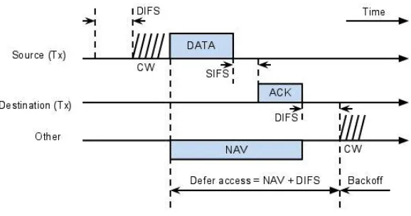
The basic Carrier Sense Multiple Access with Collision Avoidance (CSMA/CA)

mecha-nism is shown in Figure 2.1. A station desiring to transmit a frame senses (with the help

of the Clear Channel Signal (CCA) of the PHY layer) the medium and if the medium is

idle for at least a DIFS interval then the station is allowed to transmit its frame. If the

medium is busy, the station is required to wait for a DIFS interval before contending for a transmission opportunity. This period where a station contends with other stations for

transmission opportunities is known as the Contention Phase.

Figure 2.1: The basic CSMA/CA in 802.11b/g networks

When the medium is sensed busy, every station chooses a random backoff interval

between zero and contention window. The station then needs to wait for the assigned

time slots before attempting access to the channel. This additionally delays the access to the shared medium. If a station does not get access to the medium in the first attempt,

it stops its back off timer, waits for the channel to be idle again. Once the channel is

sensed idle, the station waits for DIFS time, and starts the backoff timer. Once the timer

expires, the node accesses the medium. If a collision occurs, then the station backs off

exponentially and again starts its backoff timer.

The basic CSMA/CA mechanism cannot solve the hidden terminal problem and thus

RTS (Request to Send) and CTS (Clear to Send) mechanisms are used to solve this

(19)

stations, ’STA B’ and ’STA C’ but those latter stations cannot receive data between each

other [26]. If both of these stations sense the channel idle and send the data to the ’STA

A’, which can see both ’STA B’ and ’STA C’, collision occurs at the receiver ’STA A’.

After waiting for DIFS (plus a random back off time if the medium was busy), the sender

can issue a RTS packet. The RTS packet includes the receiver of the anticipated data

transmission and the duration of that whole data transmission. This duration specifies

the time interval necessary to transmit the whole data frame and the acknowledgment

related to it. Every node receiving the RTS now has to set its Net Allocation Vector

(NAV) in accordance with the duration field. The NAV specifies then the earliest point

in time at which the station can try to access the medium again. Following a successful RTS, CTS is sent after a SIFS interval (SIFS < DIFS). After a successful reception of

CTS, DATA and ACK follow, with the duration of SIFS between the frames [26].

Though, the basic mechanism of CSMA/CA is the same across 802.11g and 802.11b,

there are differences in some of the parameters, such as MAC frame length, preamble

duration, etc. Table 2.1 provides a summary of 802.11g MAC layer parameters. It can

be noted that, if a network consists of only 802.11g devices, then the slot time used by all

the ’g’ devices is 9 µs, which is shorter than the slot time used by 802.11b devices. This is one of the factors for higher throughput in 802.11g. The following subsection provides

strategies on how 802.11g and 802.11/802.11b devices can co-exist.

Table 2.1: MAC layer parameters of 802.11g

Parameters Values

(20)

2.2.3 Operational Modes and Protection Mechanisms

With the introduction of 802.11g standard and its support for backwards compatibility,

there are three modes of operation for communication amongst the nodes in a wireless

network. These modes of operation are pure ’b’ mode, pure ’g’ mode and mixed mode.

1. Pure ’b’ mode: In this mode, a wireless network consists only of 802.11b devices.

These devices can transmit data packets either at the maximum data rate of 11

Mbps or with a data rate of 5.5, 2 or 1 Mbps. An 802.11g access point (AP) can be

operated in this mode and only 802.11b devices can associate and send data packets. Physical layer technologies used in this mode of operation are DSSS, HR-DSSS and

ERP-DSSS/CCK.

2. Pure ’g’ mode: In this mode of operation, a wireless network consists only of

802.11g devices. For a ’g’ node or a ’g’ AP, ERP-OFDM is enabled and other

technologies such as DSSS, HR-DSSS and ERP-DSSS/CCK are disabled. Hence,

in a network with AP in a pure ’g’ mode, only 802.11g devices can associate with the AP. Since all the nodes in the network are 802.11g devices, this mode is either

known as ’g’ only mode or pure ’g’ mode. As there are only 802.11g devices,

maximum throughput is achieved in this mode compared to a pure ’b’ mode or a

mixed mode environment.

3. Mixed mode: In this mode of operation, both 802.11b and 802.11g devices can

co-exist in a single network. This is a widely used operational mode. Thus, a mixed mode 802.11g AP provides association capability to both 802.11b and 802.11g

de-vices. Since this mode of operation supports both 802.11b and 802.11g devices, both

ERP-DSSS/CCK and ERP-OFDM are enabled. Since different technologies (DSSS

and OFDM) co-exist, proper mechanism of communication is required. This

mech-anism is known as protection mechmech-anism and is explained in further paragraphs.

By providing co-existence between ’b’ and ’g’ devices, aggregate throughput is

de-graded even though protection mechanism is enabled.

802.11g devices support backwards compatibility with 802.11b devices, but they use

a different modulation scheme. Unfortunately, problems still arise in a mixed mode

environment where both b and g devices exist. In such an environment, 802.11b devices

(21)

place, 802.11b devices may transmit data during 802.11g transmissions and thereby cause

collisions in the medium.

To avoid the above problem, there are two protection mechanisms - RTS/CTS

protec-tion and CTS-to-Self protecprotec-tion. RTS/CTS mechanism refers to standard RTS and CTS

frame exchanges according to the IEEE 802.11 standard. The protection mechanism is

as follows: In a mixed mode environment, when an 802.11g device needs to transmit

data to another 802.11g device, it first sends either a CTS-to-Self or an RTS/CTS frame

using a data rate (1 Mbps) and a modulation scheme that 802.11b devices can recognize.

When surrounding 802.11b and 802.11g devices hear these transmissions, they would

up-date their NAV timers with the help of the duration value present in the CTS-to-Self or RTS/CTS frames. Thus, after the CTS-to-Self or RTS/CTS frames are used to reserve

the medium, the source 802.11g device can now transmit a data frame to another 802.11g

device by using OFDM modulation.

Figure 2.2: CTS-to-Self protection mechanism

In CTS-to-Self mode, a CTS frame is sent by the source with the receiver address

same as its own MAC address. In this CTS frame, the duration value helps other nodes

to set their NAV timers, thus protecting future 802.11g frames. Figure 2.2 [6] shows an

overview CTS-to-Self protection mechanism. One of the advantages of CTS-to-Self is

(22)

throughput compared to RTS/CTS. Table 2.2 provides a summary of three operational

modes and a comparison amongst them.

Table 2.2: Comparision of operational modes

Pure ’b’ Pure ’g’ Mixed

Technology DSSS, HR-DSSS, ERP-OFDM ERP-DSSS/CCK,

ERP-DSSS/CCK ERP-OFDM

Devices allowed Only 802.11b Only 802.11g Both 802.11b, 802.11g Data rates 1, 2, 5.5, 11 Mbps 6, 9, 12, 18, 24, 1, 2, 5.5, 6, 9,

36, 48, 54 Mbps 11, 12, 18, 24, 36, 48, 54 Mbps

Protection No No Yes

Mechanism

Three possible scenarios where the protection mechanism is enabled are as follows:

1. Protection mechanism is enabled when a 802.11 legacy device or 802.11b

(HR-DSSS) device associates with a 802.11g AP.

2. Nearby 802.11b clients or 802.11b AP transmit beacons regularly. When an 802.11g

AP scans these beacons, protection mechanism is enabled in this BSS.

3. If a nearby 802.11g AP has enabled protection mechanism, beacons from this AP

could be scanned by another 802.11g AP belonging to a BSS. The latter AP then

triggers protection mechanism in its own BSS.

2.3 IEEE 802.11n

IEEE 802.11n standard was developed to provide higher throughput, better range, better

(23)

methods to increase throughput of a wireless network. These enhancements such as

Channel Bonding, Multiple Input/Multiple Output (MIMO), and improved OFDM can

increase the data rates to 600 Mbps.

Moreover, 802.11n supports operation in both 2.4 GHz and 5 GHz bands. This is a

major benefit as it provides flexibility in designing and deploying wireless networks.

An-other major advantage is its support for backwards compatibility with 802.11a, 802.11b,

and 802.11g devices. Similar to 802.11g, protection mechanisms are used in 802.11n to

aid co-existence of 802.11n and legacy devices in a BSS. We give a brief overview of the

features and enhancements implemented in 802.11n standard in following subsections.

2.3.1 Modifications and Enhancements in PHY Layer

802.11n uses the same technology as that of 802.11a and 802.11g at the physical layer. With 802.11n, an enhanced OFDM is provided which increases both reliability and data

throughput. The enhancements in PHY layer of IEEE 802.11n standard are given below.

1. MIMO:This concept is one of the features introduced in 802.11n. This enhance-ment provides capability for 802.11n nodes to transmit and receive data

simultane-ously with the help of multiple radio antennas. There can be multiple combinations

of number of transmitters and receivers in 802.11n. M x N represents the number

of transmit antennas and receive antennas, where ’M’ represents number of

trans-mit antennas and ’N’ represents the number of receive antennas. For example, 2

x 3 represents an 802.11n device with 2 transmit antennas and 3 receive

anten-nas. Higher data throughput can be achieved with more transmitter antennas and

receiver antennas.

2. Spatial Multiplexing: This feature is an application of MIMO technology. Spa-tial multiplexing involves transmitting spaSpa-tial streams using available antennas.

Each spatial stream is a unique stream of data and both the transmitter and

re-ceiver need to be MIMO capable devices. Throughput is highly increased when

spatial streams are used. In simple words, if an 802.11n node ’A’ transmits data

to another 802.11n node ’B’ using two spatial streams, then the throughput can be

effectively doubled when compared to sending data using a single spatial stream.

According to IEEE 802.11n standard, a maximum of four spatial streams can be

(24)

3. Channel Bonding: This is a major enhancement for 802.11n devices. Previously

both 802.11b and 802.11g allowed the nodes to use only 20 MHz channels. In

802.11n, channel bandwidth can also be 40 MHz, instead of 20 MHz. This resembles

using two 20 MHz channels combined together to yield a 40 MHz channel. With

40 MHz channel, throughput is effectively increased when compared to 20 MHz

channel. This is due to the increased number of subcarriers in a 40 MHz channel

that can carry data signals to the destination. Data throughput is further increased

when channel bonding is used in combination with spatial streams. Figure 2.3 shows

channel bonding considering channel 36 and channel 40 in 5 GHz band.

Figure 2.3: 802.11n Channel Bonding

4. Improved OFDM:In an OFDM carrier signal, data is modulated into a collection

of bits or symbols [5]. Guard intervals are used in order to decrease the inter symbol

interference between OFDM symbols. Guard intervals are an overhead during data

transmissions. Higher throughput is achieved when this overhead is minimal. In

case of 802.11n, its guard intervals could be shorter (400 µs) than guard intervals of 802.11a (800µs) or 802.11g (800 µs).

With respect to frequency bands and channel availability, the 2.4 GHz band has three

non-overlapping 20 MHz bandwidth channels. 5 GHz band has 23 such 20 MHz bandwidth

channels which are overlapping. For the use of channel bonding, only one

non-overlapping 40 MHz channel is available in 2.4 GHz band. In case of 5 GHz, 12 such

(25)

2.3.2 Modifications and Enhancements in MAC Layer

We have seen that the PHY layer enhancements can increase the throughput and

re-liability. But, it is necessary to incorporate MAC layer enhancements in 802.11n in

combination with PHY layer features to sustain effective throughput gains. Following

are the MAC layer enhancements in 802.11n:

1. Frame Aggregation: With 802.11b/g devices, the maximum size of payload is

2304 bytes. Frame aggregation is a technique where the MAC layer overhead can be

significantly reduced by aggregating multiple frames together before a data

trans-mission. Frame aggregation can be achieved by either of the following:

(a) MAC Service Data Unit Aggregation (A-MSDU): The upper layer

information that is contained in the body of an 802.11 wireless data frame is

called a MSDU [5]. When multiple MSDUs are combined into single frame

and then transmitted, MAC overhead factors such as medium contention and

interframe spacing are reduced considerably.

(b) MAC Protocol Data Unit Aggregation (A-MPDU): 802.11 frame

in-cluding the MAC header, body and trailer forms a MPDU. Similar to MSDU,

multiple MPDUs can be combined into a single frame and then transmitted.

Each MPDU within the A-MPDU is directed to the same receiver address. A-MPDU enhances throughput of the network by reducing MAC overhead.

The maximum A-MPDU size in 802.11n is 64K bytes.

2. Block Acknowledgement: In case of 802.11b and 802.11g devices, each and

every data packet (other than multicast/broadcast) sent from a source node is acknowledged in the form of ACK packet from the destination node. With the

higher number of unicast frames acknowledged, MAC overhead is increased and

throughput is significantly decreased. To reduce this overhead, 802.11n uses block

acknowledgement where multiple unicast frames can be acknowledged using a single

ACK packet. This is known as Block ACK.

3. Reduced Interframe Spacing (RIFS):Wireless nodes require Short Interframe

Spacing (SIFS) in between transmissions. SIFS is used to provide a small time

(26)

SIFS interval of 20 µsec and 16 µsec respectively. With respect to 802.11n, SIFS is reduced to 2 µsec. This reduced time interval is known as RIFS. Usage of RIFS results in less overhead during transmissions yielding better throughput. Table 2.3

provides a summary of 802.11n MAC layer parameters.

Table 2.3: MAC layer parameters of 802.11n

Parameters Values

Maximum MAC frame length 8191 Bytes

Slot time 9 µs

SIFS 16µs

RIFS 2 µs

Contention window size 15-1023 slots Preamble duration 16µs

2.3.3 Operational Modes and Protection Mechanisms

To maintain backwards compatibility with 802.11b/g, 802.11n access points signal other

802.11n clients using four protection modes. Depending on the devices being associated

to this AP, one of the protection modes is set in the BSS. These four protection modes

are:

1. Greenfield Mode: In this mode, all the nodes are HT 802.11n. Since all the nodes

are ’n’ devices, high throughput is achieved with this mode. Thus no protection

mechanism is required in this mode.

2. Non-Member Protection Mode: In this mode, all the stations in the BSS must

be HT stations. Protection mechanism is enabled when only a non-HT client or a

non-HT AP is heard that is not a member of the BSS [5].

3. 20 MHz Protection Mode: In this mode, all stations in the BSS must be HT

(27)

or 40 MHz (20/40 MHz) channel. If an 802.11n client capable of working only in

20 MHz channel, associates with an 20/40 MHz AP, protection must be enabled

[5].

4. Mixed Mode: This is a commonly used mode of operation. Here, 802.11b

(HR-DSSS), 802.11g (ERP-OFDM) and HT 802.11n clients associate with an HT

802.11n AP. Since there are different PHY technologies involved in the same

envi-ronment, the protection mechanism is enabled.

For the above modes, protection mechanisms that are used are either CTS-to-Self,

RTS/CTS or Dual-CTS. Dual-CTS protection mode was introduced in 802.11n. In this

mode both RTS/CTS and CTS-to-Self frames are exchanged. In a BSS, a protection mode changes dynamically depending upon the clients associating with an AP.

2.4 Overview of Cognitive Radio

A cognitive radio (CR) is an intelligent system, which was mainly designed for efficient use of dynamically available spectrum. A cognitive radio is an intelligent wireless

com-munication system that is aware of its surrounding environment (i.e., outside world), and

uses the methodology of understanding-by-building to learn from the environment and

adapt its internal states to statistical variations in the incoming RF stimuli by making

corresponding changes in certain operating parameters in real time [8].

Wireless channels in the frequency spectrum are licensed to particular users. These

users are known as primary users. Other non-license users of the spectrum are known

as secondary users. CR technology overcomes spectral shortage problems by enabling

secondary (unlicensed) wireless devices to communicate without interfering with the pri-mary users [25]. Thus CR technology is designed for dynamic spectrum allocation. That

is, CRs provide the capacity to share the wireless channel with the licensed users in an

opportunistic way [4].

To provide dynamic spectrum allocation, cognitive radios require spectrum sensing

and rapid channel switching capabilities.

Capabilities of CRs are summarized in [4] as follows:

1. Spectrum Sensing: This is an important capability for cognitive radios. CR can

(28)

2. Location identification: Location identification is another capability of a

cogni-tive radio where it determines the location of other transmitters and then selects

appropriate parameters such as the power required and frequency allowed at its

location.

3. Network Discovery: CRs are capable of doing network discovery in order to

access resources that are reachable.

4. Fast Switching Capability: CRs switch between different channels with lesser

delay compared to an 802.11 radio.

Other advantages of CR are dynamic frequency selection, adaptive modulation

de-pending on the interoperability of the system in use, adaptive power control and switching

dynamically between different power levels. All of these features make the CR an ideal

(29)

Chapter 3 Related Work

In this chapter, we present classification and characteristics of a jammer. We review some

of the research literature on jamming attacks in wireless networks with greater emphasis

on jamming attacks with respect to 802.11g and 802.11n networks.

3.1 Classification of Jammers

A jammer is a malicious node, which transmits radio signals that interferes with

legiti-mate signals in a wireless network. A jammer can be a simple device which emits jamming

signals to disrupt the communication. They also can be devices capable of emitting

ra-dio signals with intelligence (discussed later in this section). Henceforth, we will refer to

radio signals emitted by jammers as jamming pulses. Jammers can be classified into four

basic categories [17].

Constant Jammer: In a wireless medium, a constant jammer transmits jamming

pulses continuously. An important aspect of constant jammer is its non-adherence to 802.11 MAC protocols. For example, in a wireless medium, a constant jammer starts

transmitting jamming pulses, without its need to follow 802.11 MAC protocol by waiting

for the medium to be free. Data packets in transit can be corrupted when a constant

jam-mer starts its transmission of jamming pulses. Thus, by transmitting constant jamming

pulses, the medium is always busy for the legitimate nodes. Since, a constant jammer

transmits jamming pulses continuously, energy consumption is of the higher order. This

(30)

Deceptive jammer: This type of jammer is similar to a constant jammer because

both of them constantly transmit jamming pulses. In case of deceptive jammer, the

transmitted pulses are not random. In deceptive jamming, the jammer emits regular

packets or fabricated packets, which will seem identical to a regular data packet sent by

a legitimate wireless node. Due to this behavior, all the nodes in the wireless medium will

defer their transmissions, as they will sense the medium to be busy. Since a deceptive

jammer transmits jamming pulses in the form of regular packets, the probability of

detection is lower compared to a constant jammer. Similar to a constant jammer, a

deceptive jammer consumes considerable energy and is not an energy efficient jammer.

Random jammer: Unlike a constant jammer or a deceptive jammer, random jam-mers do not transmit jamming pulses continuously. A random jammer transmits jamming

pulse for a specific duration (known as pulse duration) and then sleeps for a certain

du-ration known as silence dudu-ration. Thus, by varying pulse dudu-ration or sleep dudu-ration or

both, a random jammer achieves a variation in jamming strategy. Energy consumption

of a random jammer depends on the length of the silence duration and pulse duration.

Reactive jammer: All the above types of jammers do not consider whether the

wireless medium is busy or not. For example, a constant jammer starts its transmission

irrespective of data packets in the medium. With reactive jamming, the jammer transmits

the jamming pulse only after sensing the medium for busy status. Thus, reactive jammers sense for regular data packets in the medium and transmit jamming pulses as soon as

they find the medium to be busy. Thus data packets may be corrupted and could degrade

the overall throughput of the network. Due to its reactive nature, these jammers consume

energy based on the amount of data packets they sense and jam in the medium. There

are other types of reactive jammers. For example, some jammers react to various protocol

situations rather than just busy status.

With the above types of jammer, different jamming techniques are carried out [15]

classifies jamming techniques as follows

1. Spot Jamming: In this type of jamming, the attacker targets a specific frequency

to jam and transmits jamming pulses with its total power.

2. Sweep Jamming: With sweep jamming, the attacker sweeps across all the

fre-quencies in the band to disrupt the communication.

(31)

the same time.

4. Deceptive Jamming: Here, jamming is performed in a single frequency or with

a range of frequencies with the attacker in a deceptive mode (i.e. difficult to detect

the attacker).

3.2 Classification of Jamming Attacks

Jamming attacks can be classified [10], [17] as follows:

1. PHY Layer attacks: In PHY layer jamming attacks, jamming signals are

trans-mitted in the same channel, which is used for communication by the nodes. Due

to jamming at the PHY layer, interference significantly reduces the signal-to-noise

ratio (SNR) and thus, the performance of the network is degraded. [28] highlights PHY layer jamming attacks, where a constant jammer sends jamming pulses

tar-geting a particular frequency without following any MAC layer protocol. Reactive

jamming is also used in PHY layer attack.

[2] provides different PHY layer jamming attacks such as continuous low power jamming, bursty high power jamming and busy jamming. In each of the jamming

techniques, the total energy consumed by the jammer is calculated and compared

amongst each other. With jamming attacks, energy consumption is an important

factor, since conservation of energy by a jammer leads to longevity and effective

disruption of communication in the network.

2. MAC Layer attacks: Here, jamming attacks target various protocols in 802.11

MAC layer. For example, jamming attacks target the association and

disasso-ciation processes of a node with an AP, power management, etc. In MAC layer

attacks such as deauthentication and disassociation attacks, the attacker spoofs the deauthentication and disassociation message packets and attacks a single wireless

station in the network by denying association with the AP.

[3] focuses MAC layer attacks such as disassociation and deauthentication attacks.

All the wireless nodes are required to associate (after authentication process) with an AP in the BSS for data communication. In disassociation attack, the attacker

(32)

association process. This will disassociate the node with the AP, thereby leading to

a link failure. Similarly, when a node authenticates itself with an AP, an attacker

can spoof deauthentication frame and deny association with the AP. Another type

of attack is the power saving attack [3]. Here, the attacker spoofs messages related

to power conservation functionality of a node.

3. Intelligent attacks: In this type of attack, the jammer continuously listens to

the medium and transmits jamming pulses with the knowledge of the protocol [2].

The jammer is designed with a capability to analyze the type of packet (controls

packets or data packets) and jam accordingly.

[26] provides intelligent jamming attacks which are more efficient in terms of

jam-mer’s power consumption and lower probability of detection. Intelligent jamming

attacks [26] target specific aspects of the protocol such as CTS/RTS, ACK, data

corruption jamming and DIFS wait jamming. Goals of intelligent jamming [17] include maximized jamming gain, targeted jamming and reduced probability of

detection.

4. Greedy Behavior attacks: In this type of attack, a single node or multiple nodes

behave selfishly in order to gain a higher throughput in the network. For example, a

selfish node need not follow the backoff mechanism of 802.11 CSMA/CA protocol.

Thus, a selfish node gains an unfair advantage by increasing its performance at

the cost of other nodes. [27] provides jamming vulnerabilities in 802.11e by using

misbehaving (greedy behavior) nodes in the network.

[11] and [12] also provide example scenarios of selfish nodes intending to gain higher

throughput when compared to the other nodes in the network.

3.3 Overview Jamming Attacks in 802.11g and 802.11n

As discussed earlier intelligent jamming attacks target specific aspects of the protocol

such as CTS/RTS, ACK, data corruption jamming and DIFS wait jamming. [26] provides

intelligent attacks in 802.11b which can directly be applied to 802.11g networks. By using

intelligent jamming attacks, [26] achieves maximized jamming gain, targeted jamming

(33)

[7] focuses on the effects of interference in wireless networks. For 802.11g, [7] shows

that, though 802.11g networks provide high data throughputs, small interference in the

channel considerably degrades the performance. In [9], 802.11b/g WLAN usability under

jamming is analyzed theoretically. [9] shows that, when an 802.11g system is exposed to

single carrier jamming, its performance depends highly on the jamming frequency.

[18] emphasizes that the effect of jamming depends on the number of orthogonal

channels available for use and the frequency separation between these orthogonal bands.

Depending on these two factors, a jammer in one of the channel causes interference not

only in that particular channel but also in the adjacent channel. In [18] experiments

were conducted on 802.11a and 802.11g networks and the impact on performance due to jamming was studied. 802.11g networks had lower degradation in performance when

compared with 802.11a networks. This is because orthogonal channels in 802.11g

(work-ing in 2.4GHz band) had larger channel separation compared to the channel separation

between orthogonal channels in 802.11a (5 GHz band).

A general approach to using cognitive radios to launch jamming attacks on multiple

channels of wireless networks was presented in [22]. They examine the number of channels

or users blocked by simple constant periodic jamming attacks using TCP traffic while

varying the channel switching delay, jamming packet sizes and the number of users on

the channel. We look at this in more detail, incorporating our approach in chapter 4. With respect to 802.11n, [19] provides details on jamming effects on 802.11n networks.

Here, 802.11 indoor testbeds are used to study the impact of the jammer that resides

on channels that are orthogonal to the one used by the actual nodes for legitimate

com-munication. Then they analyze the results of 802.11b/g/n networks under this jamming

condition. Results suggest that 802.11n is more vulnerable than 802.11b or 802.11g

net-works. Their observation on 802.11n is that a jammer working on an adjacent orthogonal

channel to a communication link affects the transmission of data packets in that link.

With channel bonding in 802.11n the impact of the jammer on the network is further

in-creased because channel bonding starts to eliminate orthogonality. Their results indicate that frequency hopping would not be a feasible option to mitigate jamming attacks in

802.11n networks with channel bonding. This is because channel bonding results in fewer

available channels to hop and the jammer affects the legitimate communication from an

adjacent orthogonal channel.

(34)

performed by targeting the management frames. In 802.11n management frames such

as beacon frames, action frames etc. are not encrypted in the medium. Hence, they are

susceptible to DoS attacks. These two new MAC layer attacks exploit the weaknesses

of 802.11n standard and are referenced as quiet attack and channel switch attack. A

node can send channel switch announcement frames to all other nodes when the channel

measurement reveals that the channel already in use needs to be switched. This

an-nouncement frame consists of the new channel number and a time limit within which

the channel change should take place. An attacker spoofs by providing invalid channel

number to switch or provides a larger time limit, in which case the nodes will remain

silent for that period until they switch channels. [10] also provides two other MAC layer attacks - DELBA attack and ATIM attack in 802.11n.

The DELBA attack exploits the block acknowledgement, which has been introduced

in 802.11n. The sender node sends an add block acknowledgment (ADDBA) request

which provides buffer size and the starting sequence number of the data stream [10]. The

receiver sends an ADDBA response and may adapt the buffer size to its capabilities.

The sender node sends multiple data packets and requests block ACK from the receiver.

In the tear down phase, the sender sends a delete block acknowledgement (DELBA)

message, which ends the communication, and frees the buffers of sender and receiver.

Authors in [10] propose forgery of the DELBA message. The DELBA message terminates block acknowledgement communication and frees buffers on sender and receiver side. By

impersonating the sender in an already established block acknowledgement process, the

block acknowledgment process between two stations can be terminated prematurely this

way. This frees allocated resources and will also drop all packets received so far.

Wireless nodes sleep to preserve their battery consumption. An announcement traffic

indication message (ATIM) provides an indication whether data is intended to be sent to

the node after they wake up from the sleep state. In ATIM attack, by forging the ATIM

message, an adversary can force all or specific stations to always stay awake.

[24] provides experimental studies on 802.11n. The primary focus of [24] is to present 802.11n physical and MAC layer features and study their effectiveness in different cases

such as adjacent channel interference, presence of 802.11g node, etc. 802.11n links are

degraded in the presence of 802.11g nodes. Also, though use of 40 MHz bandwidth

increases throughput, [24] presents scenarios where the presence of interference in 40

(35)

[23] focuses on how narrowband interference can be mitigated via multi-antenna

tech-niques at the receiver. Here, jamming pulses are transmitted in a particular channel to

study the effects of jamming. Nodes in this channel use multi-antenna techniques to

increase the throughput. [23] shows that multi-antenna techniques can be used to reject

narrow band jammers. It is possible to sustain a high throughput communications link

in the presence of a narrowband interference source.

The authors of [14] study how an intelligent adversary can disrupt MIMO

commu-nication by targeting the channel estimation procedure. MIMO systems require channel

state information (CSI). [14] analyzes the vulnerabilities associated with jamming the

CSI estimation procedure. CSI refers to known channel properties of a communication link. This information describes how a signal propagates from the transmitter to the

receiver and represents the combined effect of, for example, scattering, fading, and power

decay with distance. By attacking only the CSI, the jammer remains fairly covert and

power conservative as the jammer only needs to operate during a small fraction of user

transmission time. Our approach is different from [14] because, the authors jam the CSI,

which is jamming before any data packets are in the medium. In our case, we

intelli-gently jam the packets in the medium by dynamically adjusting jamming activity using

a cognitive radio.

For a DoS attack directed towards the wireless client, [21] focused on monitoring the effective throughput and stability of 802.11n and 802.11g. The DoS attack under

consideration is packet flooding [PHY layer]. This cannot be classified as a MAC layer

attack as there is no exploitation of control or management frames. Although this is a

less-intrusive DoS attack method, [21] focuses on the effectiveness of MIMO architecture

against DoS attacks. [21] compares the impact of DoS attack on throughput for 802.11n

and 802.11g networks.

[7] highlights effects of interference in 802.11b/g/n networks. With respect to 802.11n,

small amounts of interference can cause significant performance degradation of the

net-work. In [16], an anti-jamming system has been developed for 802.11 networks. [16] examines that, although 802.11n consists of MIMO, they present the same

vulnerabili-ties as that of 802.11g links in the presence of a jammer. This is due to the fact that

802.11n still employs CSMA/CA and as a result the jamming signals can render the

(36)

Chapter 4 802.11g Jamming Attacks using

Cognitive Radio

We have implemented jamming scenarios for 802.11g using a model of a cognitive radio as

a jammer [20]. We provide the simulation setup along with different jamming scenarios and evaluate their results.

We have used OPNET v16 and v16.1 modeler for network simulation. The following

sections provide the initial jamming model, description of each 802.11g jamming scenarios

and their results.

4.1 Simulation and Jamming Models

We have used the 802.11 wireless LAN model from OPNET v16. For our simulation study, we extended the wireless LAN model from [1] but with the network and transport

layers removed. Inclusion of network and transport layers will exaggerate the effects of

jamming attack and hence we have not used them in our simulations. We have heavily

modified this OPNET model for our simulation study. To study the effects of jamming

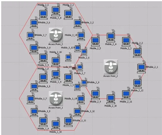
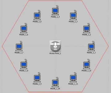
on network throughput, we used the scenario shown in Figure 4.1.

For our simulation, we have three separate networks, each consisting of 12 wireless

nodes and an AP. The AP relays messages between the twelve nodes on one network and

is shown to be a bottleneck. Each node in the network sends data packets randomly to

the other eleven nodes through the AP. The three networks are essentially independent

(37)

Figure 4.1: Base scenario model with jammer

Figure 4.2: Channel allocation for three networks

the overview of the base setup with respect to the channel usage by the three networks.

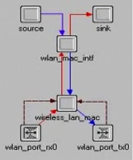
In OPNET, a wireless node model uses a source and sink module to simulate the

higher layers (IP, TCP, Application, etc.). Our source model generates packets sent

to random destination addresses. The packets received at the destination nodes are

discarded at the sink module [26]. The OPNET node model for a wireless workstation

is given in Figure 4.3.

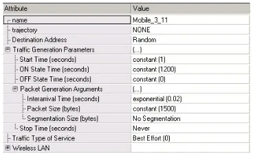
Figure 4.4 shows the wireless attributes such as channel number, data rate, etc. of

(38)

Figure 4.3: OPNET node model for wireless workstation

as its physical characteristics. We set the data rate to 18 Mbps but also consider other

bandwidths in our simulations which are shown later in this chapter.

Figure 4.4: Attributes of wireless workstation

In our scenarios, we assume all three networks to be pure ’g’ networks. Thus, there are

no 802.11b stations in any of the networks. If 802.11b devices are present, the jamming becomes significantly more effective. The majority of the simulations will be carried out

for the BSS only. Early results will show that both the CTS-to-Self and the RTS/CTS

(39)

Figure 4.5: Traffic generation parameters of a wireless workstation

these cases essentially zero. Hence, the primary set up consists of pure g devices as both

CTS-to-Self and RTS/CTS options are not set. All nodes follow the standard CSMA/CA

mechanism.

The traffic generation parameters of a wireless station node are shown in Figure 4.5.

The packet size is constant 1500 bytes with packet interarrival time of exp(0.02) seconds.

These traffic generation parameters are used for all nodes in all three networks. All

packets are sent to the AP and then relayed to a random node. We can easily see that

this load saturates the network. The offered load for each network of 12 nodes is:

(1500 + 28 header) * 50 pkts/sec. * 8 bits/byte* 12 nodes = 7.33 Mbps.

Since, this offered load must be sent to the AP and the AP must relay to the

destina-tion node, the net offered load becomes nearly 15 Mbps. Many of the scenarios considered

use the nominal 802.11g bps rate of 18 Mbps.

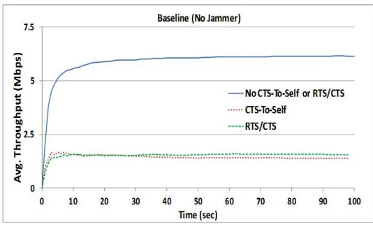
We measure the throughput for any of the networks to be just over 2 Mbps and over 6 Mbps for the sum of the three networks as given in Figure 4.6. As we mentioned earlier,

all the packets are sent to the AP and then the AP sends these packets to the destination

nodes. Thus, AP is a bottleneck and the overall throughput of each network is nearly

halved. Figure 4.6 provides a baseline throughput without the jammer. It should be

noted that baseline throughput with protection mechanisms is lower due to the overhead

of CTS-to-Self and RTS/CTS frames.

For our simulations, we have modified the single band jammer from OPNET v16.

Figure 4.7 shows the attributes of the single band jammer. This jammer module is

modified such that jamming packets are transmitted separately and at different times on the three orthogonal channels.

(40)

Figure 4.6: Baseline throughput total for three networks with no jamming

Figure 4.7: Attributes of jammer

MHz and 2462 MHz respectively. Using our jammer, we attack the center of these channels with a narrow jammer bandwidth of 1/10th of the total channel bandwidth

(20000 KHz). Thus, base frequency of the jammer is set as 2411 MHz for channel 1 with

a jammer bandwidth of 2000 kHz. The jammer is designed such that it switches to 2436

MHz (for channel 6) again with a jammer bandwidth of 2000 kHz and 2461 MHz (for

channel 11) and then backs to channel 1. This cycle of channel switching occurs until

the end of the simulation. The power of the jammer is set to 0.001 W. During our study,

we also varied the jammer bandwidth in each of the channels. We varied the jammer

bandwidth from 1000 KHz to 20000 KHz and found that the effect on throughput remains

the same for different jammer bandwidth values with constant power of 0.001 W. In the following sections, we provide two types of multi-network jamming: 1) periodic

and exponential multi-network jamming and 2) reactive and intelligent multi-network

jamming. We have assumed our cognitive radio based jammer has a channel switching

(41)

Thus, with jammer packet delay of 100 µs within the channel and with an additional 400 µs of channel switching delay, periodic jamming takes 500 µs per channel from the jamming on the earlier channel.

We show by analysis that periodic jamming (500 µs per channel) of 1500 B packets (requires 747 µs for a complete transmission) should reduce the throughput to approxi-mately 25% of the original throughput. With 802.11g networks, basic timing parameters

are:

1. 802.11g SIFS = 10 µs.

2. 802.11g fast slot time = 9 µs. This fast slot time is used only when there is a pure ’g’ network without any 802.11b devices.

3. 802.11g DIFS = 2 x Slot time + SIFS.

4. As mentioned earlier, 802.11g transmissions consist of series of symbols. At 18 Mbps, each symbol encodes 72 bits. Thus, for packet size of 1500 bytes along

with header of 36 bytes, a total of 12288 bits can be encoded in 170 symbols.

Transmission time of each symbol is 4 µs.

5. Each packet requires a 20 µs header before transmission to synchronize the re-ceiver. Also at the end of each packet, 6 µs is added for signal extension to provide backwards compatibility.

Each network receives a jamming signal on average every 1500 µs. For example, the jammer intially attacks channel 1 and takes on average 1500µs to come back to channel 1 for attacking this network.

The complete transmission time for a packet size 1500 B is provided in the Table

4.1. Because of the additional collisions generated, the expected reduction in throughput

should be even more than caused by jamming. Our results in the following sections provide a reasonable verification for our work.

Thus, with 747 µs as the total time for transmitting a 1500 B packet and jammer transmits a jamming pulse on each network on average every 1500 µs. An approximate probability is given by

(42)

Table 4.1: Timings of transmitting a 1500 byte packet in pure ’g’ network

Data Details

DIFS 28µs (2*9) + 10

Data 709 µs 20 + (4 * 170) + 6 SIFS 10µs SIFS for 802.11g = 10 µs Total 747 µs 28 + 709 + 10

The actual jamming can occur prior to the data being sent and hence the total time of the effect of the jamming will be slightly less than the 747 µs. However 677 µs is attributed to the transmission of the packet itself.

Thus,

P(1500 B pkt in transmission not to be hit by jamming packet) =

1−P(Jammer packet hitting a 1500 B pkt in transmission) = 0.502

Since packets are transmitted from a source node to AP and then the AP to the

desti-nation node,

P(Successful transmission of 1500 B packet) =

P(Successful transmission of 1500 B packet from source to AP)

∗ P(Successful transmission of 1500 B packet from AP to destination) = = 0.502∗0.502

= 0.25

(43)

4.2 Periodic and Exponential Multi-Network

Jam-ming

In this section, we provide simulation results for periodic and exponential jamming

at-tacks. For all attacks presented here, the jammer is not required to be a part of the

targeted network but needs to be able to sense transmission energy in the appropriate

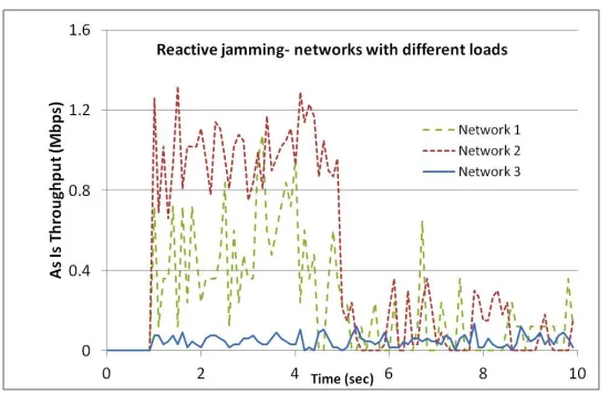
frequency. For these attacks, a short jamming pulse is transmitted that causes interfer-ence or makes the network appear busy. We label networks running on channel 1, 6, and

11 as N1, N2, and N3 respectively.

The CR acts as a jammer sending a short pulse (8 bits) on N1, then switches to N2 and

then switches to N3 to complete one cycle. As mentioned earlier, we have assumed the

switching delay between networks to be 400 µs based on the fast switching capability of a CR. This is incorporated in the modified version of our jammer module. The jammer

starts transmitting packets five seconds after the start of the simulation. A general

algorithm for periodic and exponential jamming is provided in Algorithm 1. Appendix

A provides the jammer code module modifications required for periodic and exponential

jamming.

Our first jamming scenario consists of periodic jamming attacks with constant and

exponential delays after the jammer switches to the new network. We consider two values

a) 100µs and b) 400µs for each case of constant delay and exponential delay. This value is modified in ’Jammer Packet Interarrival Time’ of the jammer attributes. Along with

the jammer packet interarrival time, we also add the channel switch time. Thus, the

simulation was done with 100 µs and 400 µs plus the 400 µs channel switch time as the time between jamming transmissions. Effect of periodic jamming attack with constant

and exponential delay is shown in Figure 4.8. Constant delay instead of exponential

(44)

Figure 4.8: Constant and exponential periodic jamming

Algorithm 1: Periodic and Exponential Jamming

Data: Jammer attributes: base frequency, bandwidth, etc.;

Set base frequency to 2411 ; /* Set the base frequency (MHz) to ch1 */

Set bandwidth to 2000 ; /* Set the narrow jammer bandwidth (KHz) */

Set channel switch delay to 400 ; /* Set CR channel switch delay (µs) */

while simulation duration not expired do

sendJammingPkt () ; /* Sends jamming packet in ch 1 */

wait for channel switch delay

Add 25 to base frequency ; /* Switch to center frequency ch 6 */

Add 25 to base frequency ; /* Switch to center frequency ch 11 */

switch to channel 1 ; /* Switch to center frequency of ch 1 */

end

(45)

However, periodic jamming with constant intervals would be easily detected and

the nodes could adjust their transmission patterns to evade the jammer and optimize

throughput. Thus, all scenarios after Figure 4.8 are conducted with exponential jammer

delays.

Figure 4.9: Instantaneous - exponential jamming at 18 Mbps with 10 iterations. Each color represents one of the 10 iterations with different random seeds.

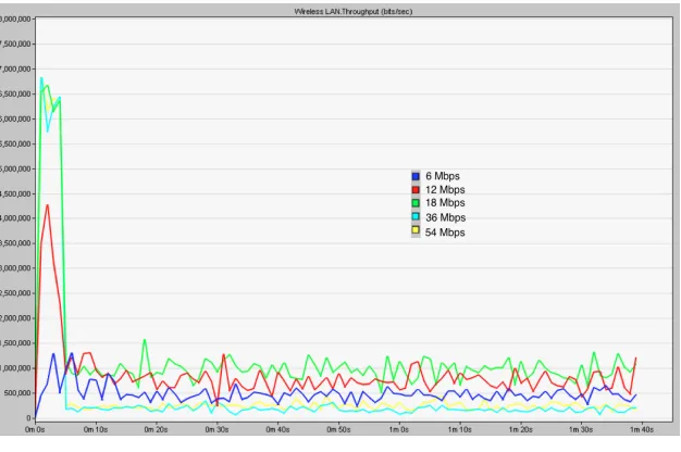
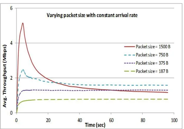
802.11g devices can communicate in the distinct data rates of 6, 9, 12, 18, 24, 36,

48 and 54 Mbps. In this scenario, we show the effects of our jamming attack and the

degradation in throughput at five of these different data rates. This simulation uses

the base scenario with all nodes generating 1500 bytes packets with interarrival rate of

exp(0.02) seconds. All the jamming scenarios in this section were run for 10 iterations with different random seeds. Figure 4.9 shows 10 iterations with different random seeds

for exponential jamming at 18 Mbps. We have shown a snapshot from the OPNET

simulation to provide results with better clarity. While Figure 4.9 shows instantaneous

throughput result, Figure 4.10 shows average throughput result for the same scenario.

With 10 iterations, Figure 4.11 and Figure 4.12 present 95% confidence interval for

exponential jamming at 18 Mbps for instantaneous and average throughput respectively.

Signal-to-Noise Ratio (SNR) is a critical factor when data is transferred with different

data rates. This is due to the fact that the data rates have different underlying modulation

techniques. Greater SNR is required for more efficient modulation techniques (QAM-64), but less efficient modulation techniques such as BPSK tolerate lower SNR and therefore,