Kinetic Nucleation Theory and Thermal Fluctuations in the Formation of Cosmic Dust.

(1)

Abstract

FALLEST, DAVID WILLIAM. Kinetic Nucleation Theory and Thermal Fluctuations in the Formation of Cosmic Dust. (Under the direction of Davide Lazzati.)

Large amounts of dust (_∼ 108 _M

) have been observed in quasi-stellar objects at high-redshift (z > 5), but the origin of such dust is still a mystery. Most dust

forma-tion models rely on classical nucleaforma-tion theory which treats nucleaforma-tion in condiforma-tions of

thermodynamic equilibrium. A theory of nucleation based on the kinetic theory is

devel-oped here incorporating non-local thermodynamic equilibrium and taking size dependent

grain properties into account. The kinetic theory of nucleation, while computationally

more expensive than classical nucleation theory, provides an improved methodology for

determining nucleation rates of dust grains, and is well suited for predicting dust yields from astronomical sources. In this improved theory, size dependent grain properties, such

as grain shape and binding energy, rather than bulk material properties as in classical

nucleation theory, are used whenever possible. Additionally, Monte Carlo methods are

employed to evolve the size of the grain and to determine its temperature fluctuations due

to collisional heating from monomer attachment and carrier gas interactions. The

evap-oration rate of a grain depends sensitively on its temperature, an effect not considered in

classical nucleation theory. An average detachment rate is calculated for each initial grain

size, and attachment and detachment rates as a function of grain size are found.

Nucle-ation rates are calculated from the attachment and average detachment rates. Grain sizes and temperatures as a function of time are presented for two sample materials: water

and carbon. Nucleation rates for water droplets are found for saturation levels in the

range from 6 to 30 and compared to expansion cloud chamber experiment results. Dust

mass yields of carbonaceous grains are calculated and compared with previous dust mass

(2)

c

(3)

Kinetic Nucleation Theory and Thermal Fluctuations in the Formation of Cosmic Dust

by

David William Fallest

A dissertation submitted to the Graduate Faculty of North Carolina State University

in partial fulfillment of the requirements for the Degree of

Doctor of Philosophy

Physics

Raleigh, North Carolina

2012

APPROVED BY:

Stephen Reynolds Lubos Mitas

Tarek Echekki Davide Lazzati

(4)

Dedication

To my family and friends, in Illinois, Wisconsin, North Carolina, or wherever you are,

for your continued support throughout the whole graduate school process.

(5)

Biography

David Fallest was born in Chicago, IL, in 1974 and grew up in Des Plaines, IL. While being

considered an intelligent child, David did not enjoy attending school. After graduating

from Elk Grove High School in 1992, David spent some time at the University of Illinois at

Chicago studying architecture. However, still disillusioned with the educational system,

in 1994 he left UIC to pursue life in the “real world” instead. At the time, David was

given a choice by his father: go back to school or start paying rent. In order to avoid paying rent, David chose to continue his education, but only taking those classes that

interested him, mainly, math and science. This was probably the best decision he ever

made.

Throughout the next seven years David slowly worked his way through his associate’s

degree at William Rainey Harper College. During this time David also worked as an

apprentice and journeyman electrician with I.B.E.W. Local 134 in Chicago, IL, and

noo-dled around as a juggler and variety performer. In 2002, David graduated from Harper

College, and enrolled at Beloit College in Beloit, WI. In 2006, David graduated from

(6)

Acknowledgements

Special thanks to Dr. Davide Lazzati for his guidance, wisdom, and never-ending patience.

Thanks also go to Dr. Takaya Nozawa and Dr. Ken’ichi Nomoto for allowing me to

conduct part of this research at the Institute for the Physics and Mathematics of the

Universe in Kashiwa, Japan.

Finally, I would like to thank Drs. Umeda and Nomoto for allowing me to use their

(7)

List of Tables

Table 3.1 Carbon properties . . . 39

Table 3.2 Total mass of carbon grains formed . . . 49

Table 4.1 Physical properties of H2O water. . . 71

Table 4.2 TemperatureT and corresponding water vapor fractionsω. . . 72

Table 4.3 Critical cluster sizes for all simulations using the modified kinetic nucleation theory with 2000 detachments (except where noted oth-erwise). . . 79

Table 4.4 Nucleation rates for all simulations using the modified kinetic nu-cleation theory for cluster sizes up to 2n∗ and 2000 detachments. . 81

Table 4.5 Critical cluster sizes and nucleation rates for increasing argon carrier gas pressures. . . 84

Table 4.6 Physical properties of carbon (graphite). . . 87

(10)

List of Figures

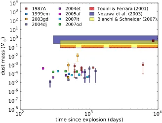
Figure 1.1 Total dust masses inferred from observations of CCSNe (see Gall et al. (2011) and references therein). Filled squares represent in-ferred total dust masses. Error bars are included for observations that infer a range of total dust mass values and the filled square was placed at the center of the range. Observations that inferred a range of dust mass values over the span of a number of days are shown as filled areas. Also shown are the overlapping ranges of pre-dictions of total dust masses for the models of Todini and Ferrara (2001) for SN1987A with dust formation starting as early as day 380, Nozawa et al. (2003) for 13–40 M progenitor stars with dust forming as early as day 300, and the revised model of SN1987A by Bianchi and Schneider (2007). . . 3 Figure 1.2 Milky Way Galaxy (Brunier, 2008). The dark patches running

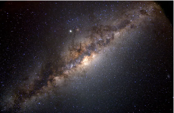
through the middle of the galaxy were once thought to be areas devoid of any material, allowing one to see beyond the galaxy. . . 4 Figure 1.3 Composite x-ray image of SNR Cas A (Stage et al., 2006) taken

using NASA’s Chandra X-ray Observatory. The red, green and blue colors correspond to 0.5–1.5 keV, 1.5–2.5 keV, and 4.0–6.0 keV X-ray energies, respectively. . . 5 Figure 1.4 Composite image of SN1987A from the Hubble Space Telescope.

(NASA et al., 2007) . . . 6 Figure 1.5 Isomers of C24 found using density functional theory techniques

(Jones, 1999). . . 7

Figure 2.1 Free energy of a system in relation to its volume. For the system to transition from the metastable state to the stable state, it must overcome an energy barrier. . . 11 Figure 2.2 Dimensionless Gibbs free energy as a function of reduced volume . 13 Figure 2.3 Gibbs free energy minima as a function of supersaturationS. . . . 14 Figure 2.4 A system ofM monomers before and after cluster formation (replica

of Fig. 3.2 from Kashchiev (2000)). . . 15 Figure 2.5 Change in Gibbs free energy as a function of cluster size. . . 17 Figure 2.7 Fig. 1 from Oxtoby and Evans (1988). Density profile for a critical

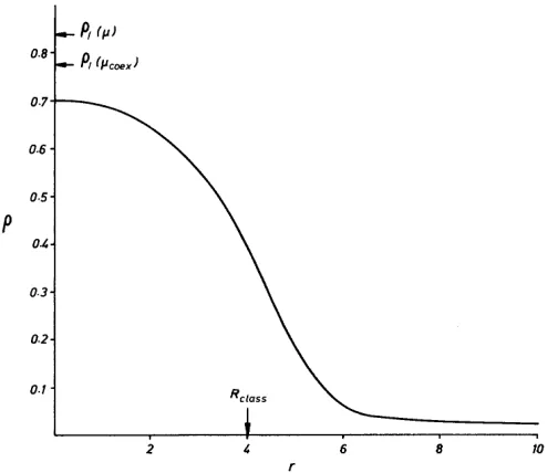
cluster at T0 = 0.6. ρl(µ) is the liquid density at this T0, ρi(µcoex)

is the liquid density when the liquid and vapor can coexist, and Rclass is the radius of the classical critical cluster. . . 24

(11)

Figure 2.9 (a) Fig. 3 from (Kalikmanov, 2006) comparing nucleation rate found using CNT (open circles) and MKNT (filled circles) for argon. (b) Fig. 7 from (Kalikmanov, 2006) comparing nucleation rates found using CNT (open circles and squares) and MKNT (filled circles and squares) for water. The open circles correspond to the work of W¨olk and Strey (2001). . . 27

Figure 3.1 Density evolution for 4.96 (black) and 6.0 (red) M enclosed mass subshells up to 1000 days after the SN explosion. . . 40 Figure 3.2 Temperature evolution for 4.96 (black) and 6.0 (red) M enclosed

mass subshells up to 1000 days after the SN explosion. . . 41 Figure 3.3 Number fraction of helium (green dash-dot), carbon (black dashed),

oxygen (red dotted), and silicon (magenta dash-dot) atoms for en-closed masses from 2.45 to 8.7 M. The solid (blue) line is the carbon number fraction after the formation of CO molecules. . . . 42 Figure 3.4 Nucleation rates for spherical grains ( c = (36π)1/3), for the four

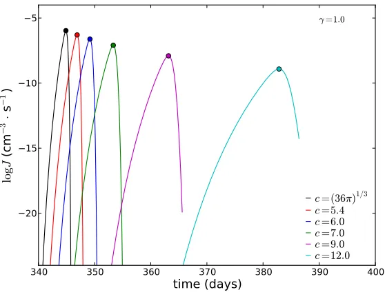
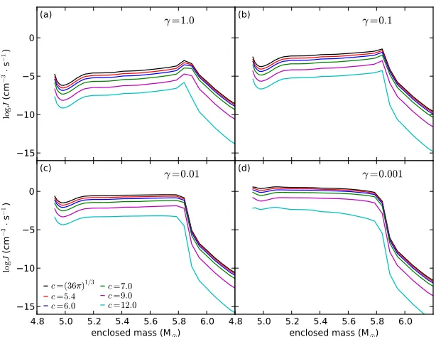
considered sticking coefficients of γ = 1.0, 0.1, 0.01, and 0.001. Filled circles indicate the time and rate of maximum nucleation. Rates are calculated at an enclosed mass coordinate 4.96M. . . . 44 Figure 3.5 Maximum nucleation rates for spherical carbon grains at enclosed

masses <6.2 M for four sticking coefficients. . . 45 Figure 3.6 Nucleation rates for spherical carbon grains at an enclosed

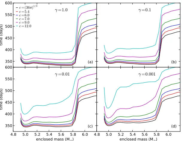
coordi-nate of 6.00 M for four sticking coefficients. Condensation times are indicated by filled circles. . . 46 Figure 3.7 Condensation times of spherical carbon grain as a function of

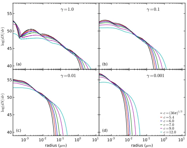
en-closed mass for four sticking coefficients. . . 47 Figure 3.8 Size distribution of carbon grains for γ = 1.0, 0.1, 0.01, 0.001,

with c = (36π)1/3. For reference, the solid (red) line represents the power-law distribution with the form of Nr ∝ r−3.5, which

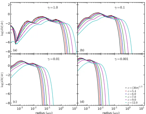
has been suggested as that of interstellar grains (e.g., Mathis et al. (1977)). . . 48 Figure 3.9 Mass distribution of carbon grains for γ = 1.0, 0.1, 0.01, 0.001,

with c= (36π)1/3_{. . . .} ₄₈

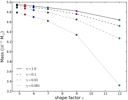
Figure 3.10 Nucleation rates as a function of time for six shape factors with γ = 1.0. Filled circles indicate maximum nucleation rate. Rates shown are for nucleation within a shell of enclosed mass of _∼4.96 to_∼4.97 M. . . 50 Figure 3.11 Maximum nucleation rates for all six shape factors and four sticking

coefficients. . . 51 Figure 3.12 Dust condensation times for six shape factors and four sticking

(12)

Figure 3.13 Size distribution of carbon grains for six shape factors and four sticking coefficients. . . 53 Figure 3.14 Mass distribution of carbon grain for six shape factors and four

sticking coefficients. . . 54 Figure 3.15 Total mass of carbon dust formed for all simulations. . . 55 Figure 3.16 Total mass of dust formed for spherical carbonaceous grains with

sticking coefficients down to γ = 10−9_. _{. . . .} ₅₅

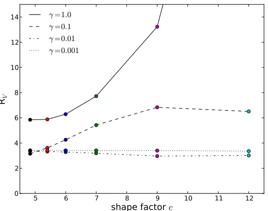
Figure 3.17 Extinction curves for each sticking coefficient and shape factor. . . 56 Figure 3.18 RV values for 23 simulations. Not shown is RV = 41 for c= 12.0

and γ = 1.0. . . 56

Figure 4.1 Detachment rate ˜gn (Eq. (4.9) vs. cluster temperature for an n =

100 water cluster. . . 65 Figure 4.2 Sublimation energies for water clusters calculated from Eq. (4.19)

(shaded grey region), the data of Lenz and Ojam¨ae (2009) (blue, filled circles), Shank et al. (2009) (red, filled square), and Wang and Bowman (2011) (black, filled square). The blue connecting lines between the Lenz & Ojam¨ae data points are a guide for the eye. The horizontal, dashed line indicates the bulk sublimation energy of water of 7.76_×10−13 _{ergs. . . .} ₇₃

Figure 4.3 Curves of b = Bn/~ω0 and m = Un/~ω0 for the dimer (n = 2)

and trimer (n = 3) clusters. Sublimation curves are found using Eqs. (4.19) and (4.36) (dashed) and from the data of Lenz and Ojam¨ae (2009) (dotted). . . 74 Figure 4.4 Attachment, unmodified detachment and the basic detachment

rates from Eq. (4.7) (dashed cyan), with temperature fluctuations (Eq. (4.9) in green), Eq. (4.7) with corrections for small grain sizes (magenta), and all modifications included, Eq. (4.31) (blue), for water droplets in a surrounding vapor atT = 240 K and S= 10. . 76 Figure 4.5 Same as Figure 4.4 except the only detachment rate shown is the

modified detachment rate found using Eq. (4.31). . . 77 Figure 4.6 Same as Figure 4.5 except the simulations are allowed to run until

clusters have undergone 10000 detachments. The nucleation rate Js is found using the last 5000 detachment events . . . 78

(13)

Figure 4.8 Critical cluster sizes for water droplets as a function of supersat-uration S for vapor temperatures of 220 (red), 230 (green), 240 (blue), 250 (magenta), and 260 (cyan) K. Sizes are found using the modified (diamonds) and unmodified (squares) kinetic nucleation theories. The connecting lines are a guide for the eye. Critical sizes found using CNT are also shown. . . 80 Figure 4.9 Nucleation rates as a function of supersaturationS for water

droplets for vapor temperatures of 220 (red), 230 (green), 240 (blue), 250 (magenta), and 260 (cyan) K. Rates are calculated using the modified (diamonds) and unmodified (squares) kinetic nucleation theories and CNT (dash-dot curves). Also shown are experimental values of W¨olk and Strey (2001). . . 82 Figure 4.10 Modified detachment rates for seven different argon carrier gas

pres-sures at a vapor temperature of 240 K and supersaturationS = 10. pAr = 146 p (blue data) corresponds to the carrier gas pressure

used in the other simulations at the same temperature and super-saturation. . . 83 Figure 4.11 Nucleation rates (black) and critical cluster sizes (blue) for

increas-ing carrier gas pressurespAr/p. . . 83

Figure 4.12 Attachment, unmodified detachment, and modified detachment rates for water droplets in a surrounding vapor at T = 240 K and S = 10 using dissociation energies of Shank et al. (2009) and Wang and Bowman (2011). . . 84 Figure 4.13 Attachment, unmodified detachment, and modified detachment

rates for water droplets in surrounding vapor at T = 240 K and S = 10 using binding energy data of Lenz and Ojam¨ae (2009). . . 85 Figure 4.14 Attachment, unmodified detachment, and modified detachment

rates for carbonaceous grains with a hydrogen carrier gas at

T = 2500 K and S= 5. . . 86 Figure 4.15 Sublimation energies for carbon clusters n= 2–55 calculated with

Eq. (4.19) from binding energy data of Kosimov et al. (2008, 2010) (blue filled circles) and found using Eq. (4.36) (gray curve). The horizontal, dashed black line is the bulk sublimation energy for graphite. . . 88 Figure 4.16 Attachment, unmodified detachment, and modified detachment

(14)

Figure 5.1 Attachment (black), basic (blue, dashed) and unmodified (red) de-tachment rates for carbon clusters at T = 2500 K and S = 5, with critical cluster size of n = 52 for the basic and unmodified detachment rates, respectively. . . 94 Figure 5.2 Nucleation rates for spherical grains, c= (36π)1/3_{, with a sticking}

coefficient of γ = 1.0 as a function of time after explosion found using CNT (black curve) and KNT (red curve) at an enclosed mass of 4.96 M. . . 95 Figure 5.3 Size distributions as a function of grain radius for grains formed

in the ejecta of a CCSN using CNT (black) and KNT (red). The distribution of interstellar grains suggested by Mathis et al. (1977) is shown in gray. . . 97 Figure 5.4 Mass distributions as a function of grains radius for grains formed

in the ejecta of a CCSN using CNT (black) and KNT (red). . . . 97 Figure 5.5 Extinction curves associated with the carbon grains predicted to

form using CNT (black) and KNT (red). . . 98 Figure 5.6 Nucleation rates for carbonaceous grains in the ejecta of a 20 M

progenitor CCSN. Rates shown are found using both CNT (black curves) and KNT (red curves) for shape factors, c = (36π)1/3 and 9.0 (solid and dashed, respectively), and sticking coefficients γ = 1.0 and 0.01 (dash-dot and dotted, respectively). . . 100 Figure 5.7 Nucleation rates for carbonaceous grains found using KNT with

Eq. (4.7) (blue) and Eq. (4.8) (red) at M= 4.96 M for shape factors c = (36π)1/3 _{and 9}_._{0 and sticking coefficient} _γ _{= 1}_._{0 and}

0.01. . . 101 Figure 5.8 Same as Figure 5.1 except with additional detachment rates found

using the carbon cluster binding energies of Kosimov et al. (2008) and (2010) (magenta). A single critical cluster size is unable to be determined. . . 102 Figure 5.9 Nucleation rates of carbonaceous grain formation at an enclosed

mass of 4.96 M. Rates shown are found using CNT (black), KNT with unmodified detachment rates (red), KNT with basic detachment rates (blue), and detachment rates including the data of Kosimov et al. (2008, 2010). All rates assume spherical grains c= (36π)1/3_{, with sticking coefficient} _γ _{= 1}_._0. _{. . . .} ₁₀₃

(15)

(16)

List of Symbols

Symbol Meaning

A kinetic prefactor of steady nucleation rate

A0 kinetic prefactor of steady nucleation rate

Bn sublimation energy of n-sized cluster

b energy quanta necessary to free a monomer from the cluster

C(n) distribution of n-sized clusters

Cexp expansion-cloud chamber droplet concentration

Cf(m) number of ways m quanta can be distributed among f degrees of freedom

Cn concentration of n-sized clusters

C0 concentration of nucleation sites

C1 concentration of monomers

C1,e monomer concentration at the phase-equilibrium pressure

C24 Carbon cluster with n= 24

˜

C1 nominal concentration of monomers

c shape factor

En binding energy of n-sized cluster

f degrees of freedom

fn monomer attachment rate to n-sized cluster

fn,Ar collision rate of argon carrier gas atoms with an n-sized cluster

f1 attachment rate of monomers onto a monomer cluster

f∗ attachment rate of monomers on to the critical cluster

i energy quanta contained in a vibrational degree of freedom

G Gibbs free energy

Gref reference energy

G1 Gibbs free energy in old phase

G2 Gibbs free energy in new phase

Gex excess Gibbs free energy

gn monomer detachment rate from n-sized cluster

gn,unmod unmodified detachment rate

g_n∗ detachment rate including cluster temperatures and rate corrections for

(17)

Symbol Meaning

˜

gn detachment rate accounting for cluster temperature

~ Planck’s constant divided by 2π J nucleation rate

JBD Becker & D¨oring nucleation rate

JCL nucleation rate found using classical nucleation theory

Jexp expansion-cloud chamber nucleation rate

JM D nucleation rate found using molecular dynamics methods

Js steady nucleation rate

˜

J nucleation rate from the self-consistent model of Girshick and Chiu (1990)

Kcg kinetic energy of a carrier gas monomer

Kcg,f final carrier gas monomer kinetic energy

Kcg,i initial carrier gas monomer kinetic energy

Kin kinetic energy of impinging monomer

Kout kinetic energy of ejected monomer

k Boltzmann constant

keV kiloelectron volt

M number of particles in the system

M solar mass

Mr enclosed mass

m energy quanta available in the cluster

mAr mass of argon atom

m0 monomer mass

N number of particles in the phase

n number of monomers in the cluster

nd number density

n∗ number of monomer in critical cluster

Pcr critical pressure

P0 reduced pressure

P_e0 reduced phase equilibrium pressure

p vapor pressure

pAr argon carrier gas pressure

(18)

Symbol Meaning

pf(b) probability a degree of freedom contains at least b energy quanta

p0 standard pressure of 1 bar

Rclass critical cluster radius found through classical nucleation theory

RV ratio of total to selective extinction

r cluster radius

ref f cluster effective radius

r∗ radius of critical cluster

S supersaturation

Sn rate correction for small grains

S entropy

T temperature

Taf ter cluster temperature after monomer detachment

Tbef ore cluster temperature before monomer detachment

Tcluster cluster temperature

Tcr critical temperature

TDebye Debye temperature

Tgas vapor temperature

Ts average temperature of water and carrier gas molecules

Tw average temperature of water molecules

T0 reduced temperature

t time of cluster volume measurement

te equilibrium time

tn time after explosion

t0 initial time after explosion

t0 time of cluster formation

U internal energy

Un internal energy of n-sized cluster

Un,f final cluster internal energy

Un,i initial cluster internal energy

U1 internal energy of monomer

V volume

(19)

Symbol Meaning

Vshell volume of expanding mass shell

V∗ volume of the critical cluster

V0 reduced volume

v0 monomer volume

v∗ volume of the critical cluster

W(n) work to form n-sized cluster

W1 work to form monomer cluster

W∗ work to form critical cluster

Xn n-sized cluster of nucleating material

X1 monomer of nucleating material

Y1 ratio of the monomer concentration to the nominal monomer concentration

Z metallicity

z redshift

zZ Zeldovich factor

γ sticking coefficient

γf mean energy quanta per degree of freedom

γ∗ size dependent sticking coefficient

∆G change in the Gibbs free energy

∆G∗ change in Gibbs free energy to form critical cluster

∆ ˜G work of cluster formation from the self-consistent model of Girshick and

Chiu (1990)

∆ ˜G∗ _{work of critical cluster formation from the self-consistent model of Girshick} and Chiu (1990)

∆Kcg change in kinetic energy of carrier gas monomer

∆texp expansion-cloud chamber nucleation time

∆Vgrains,n total change in volume of grains

∆µ change in chemical potential

λ wavelength

λsub bulk sublimation energy

µ chemical potential

µcoex chemical potential when vapor and liquid can coexist

(20)

Symbol Meaning

µold chemical potential of old phase

ρi liquid density when vapor and liquid can coexist

ρl liquid density

Σ surface area

σ surface energy/tension

Φ(n) effective excessive energy of n-sized cluster

ω water vapor fraction

(21)

List of Abbreviations

Abbreviation Meaning

AGB asymptotic giant branch

AGNs active galactic nuclei

B3LYP Becke, three-parameter, Lee-Yang-Parr

CAMS constant angle Mie scattering

Cas A Cassiopeia A

CCSN core-collapse supernova

CCSNe core-collapse supernovae

CNT classical nucleation theory

DFT density functional theory

DMC diffusion Monte Carlo

EAPSI East Asia and Pacific Summer Institute

He-Ne Helium-Neon

IPMU Institute for the Physics and Mathematics of the Universe

ISM interstellar medium

KNT kinetic nucleation theory

MC Monte Carlo

MD molecular dynamics

MEXT Ministry of Education, Culture, Sports, Science and

Technology in Japan

MKNT mean-field kinetic nucleation theory

NSF National Science Foundation

REBO reactive empirical bond-order

RRK Rice-Ramsberger-Kassel

SN supernova

SNe supernovae

SNR supernova remnant

SNRs supernova remnants

(22)

Chapter 1 Introduction

Attitudes towards dust in the cosmos have gone through dramatic changes over the

past hundred years. In the first half of the twentieth century, dust was considered to

be little more than a nuisance to observations, but by the end of the century it was

known to be vitally important to galactic evolution. Currently, cosmic dust is one of

the most interesting areas of study in astrophysics. While dust is ubiquitous in the Universe it is still poorly understood. Among the various riddles surrounding cosmic

dust are the mechanisms that lead to the formation of dust particles, and the locations

where the first grains condensed. This dissertation focuses on improving the theoretical

framework describing the dust formation process – nucleation – to include for the first

time considerations of cluster microphysical properties and temperature fluctuations. The

modified nucleation theory is developed using water droplet formation as a test case, and

is then applied to the formation of carbonaceous dust grains in the expanding ejecta of

a core-collapse supernova.

1.1 Motivation

Large amounts (_∼108 _M

) of dust have been inferred from observations of high-redshift (z > 5) quasars (Bertoldi et al., 2003; Priddey et al., 2003; Beelen et al., 2006; Dwek

et al., 2007; Wang et al., 2008). Asymptotic giant branch (AGB) stars (Morgan and

Edmunds, 2003; Zhukovska et al., 2008; Valiante et al., 2009) and core-collapse

super-novae (CCSNe) (Kozasa et al., 1989, 1991; Todini and Ferrara, 2001; Nozawa et al., 2003;

(23)

thought to produce the largest amounts of dust and scenarios can be constructed where

either of these sources produces the observed dust amounts (Dwek and Cherchneff, 2011).

Arguments have been made, however, that since the age of the Universe at that redshift

was less than one gigayear, AGB stars have not had sufficient time to evolve off the

main sequence and to produce much dust (Dwek, 1998). Therefore, supernovae (SNe)

of massive, short-lived Population III stars would be the most likely source of the dust

(Bromm et al., 2002; Morgan and Edmunds, 2003; Maiolino et al., 2004; Dwek et al.,

2007). Unfortunately, such SNe are not observable with current instrumentation.

There-fore, we must rely on theoretical predictions of dust yields from these SNe to determine

if they could, indeed, be the dominant source of high-redshift dust.

Dust production predictions must then necessarily be compared against observations

of recent SNe, such as SN1987A, and supernova remnants (SNRs), such as Kepler and

Cassiopeia A (Cas A). Unfortunately, the accuracy of these predictions is suspect.

Dis-crepancies as large as three orders of magnitude occur between total dust masses

pre-dicted theoretically and those inferred from far-infrared and submillimeter observations

(see Figure 1.1). This implies that the theory used for making dust formation

predic-tions needs to be reconsidered, and alternatives developed, in order to improve or confirm

current dust predictions, and ultimately, to determine the origin of dust at high-redshift.

1.2 Dust in the cosmos

We now know that approximately one percent of the interstellar material in our own Milky

Way galaxy consists of dust particles (Bussoletti and Colangeli, 1990). Before the early

twentieth century, however, astronomers did not know dust existed. In the late eighteenth

century, dark patches observed in the Milky Way (see Figure 1.2) led astronomers to

believe that these patches were actually areas devoid of any material (Herschel, 1785).

Later, observations indicated that the light from a distant object suffers from extinction, which allowed astronomers to figure out that there must be some sort of intervening

material blocking part of the light (Hartmann, 1904). Finally, Trumpler (1930) showed

that some of this intervening material consisted of small solid particles – dust. Due to

its ability to hamper observations, the fog of dust caused accurate calculations to distant

objects to be problematic (Dorschner and Henning, 1995; Li and Greenberg, 2003). It

(24)

10

2

₁₀

3

₁₀

4

time since explosion (days)

10

-8

10

-7

10

-6

10

-5

10

-4

10

-3

10

-2

10

-1 0

10

1

10

2

10

3

10

4

du

st

m

as

s (

M

¯

)

1987A

1999em

2003gd

2004dj

2004et

2005af

2007it

2007od

Todini & Ferrara (2001)

Nozawa et al. (2003)

Bianchi & Schneider (2007)

Figure 1.1: Total dust masses inferred from observations of CCSNe (see Gall et al. (2011) and references therein). Filled squares represent inferred total dust masses. Error bars are included for observations that infer a range of total dust mass values and the filled square was placed at the center of the range. Observations that inferred a range of dust mass values over the span of a number of days are shown as filled areas. Also shown are the overlapping ranges of predictions of total dust masses for the models of Todini and Ferrara (2001) for SN1987A with dust formation starting as early as day 380, Nozawa et al. (2003) for 13–40 M progenitor stars with dust forming as early as day 300, and the revised model of SN1987A by Bianchi and Schneider (2007).

the Universe were realized: dust vigorously influences galactic evolution (Dorschner and

Henning, 1995) and enriches the metallicities of successive generations of stars (Schneider

et al., 2006), is the basis for the formation of rocky planets, is vital to astrochemistry by providing sites for the formation of molecules (Bussoletti and Colangeli, 1990; van

Dishoeck et al., 1993; Schneider et al., 2006; Cherchneff and Dwek, 2010), and polarizes

starlight (Draine, 2003). Currently, cosmic dust grains are being studied from both

observational and theoretical points of view, and dust grain analogs are being studied in

(25)

Figure 1.2: Milky Way Galaxy (Brunier, 2008). The dark patches running through the middle of the galaxy were once thought to be areas devoid of any material, allowing one to see beyond the galaxy.

Draine (2003) identified nine, and Li and Greenberg (2003) fifteen, problems about

cosmic dust that still do not have satisfactory answers. One of the questions raised

by Li and Greenberg is “what are the sources and sinks (destruction) of interstellar

dust?” Dust sources include molecular clouds, galaxies, active galactic nuclei (AGNs)

and quasars (Dwek et al., 2007), colliding wind regions of binary systems including Wolf-Rayet stars (Cherchneff, 2010), mass loss winds of AGB stars (Morgan and Edmunds,

2003; Zhukovska et al., 2008; Valiante et al., 2009), and the ejecta of SNe and SNRs

(Kozasa et al., 1989, 1991; Todini and Ferrara, 2001; Nozawa et al., 2003; Bianchi and

Schneider, 2007; Kozasa et al., 2009; Cherchneff, 2010; Nozawa et al., 2011). However,

how efficient any of these sources are at creating dust is as yet unknown.

1.2.1 Dust at high-redshift

One issue being debated is the source of dust at high-redshift (z > 5). As an example,

let us consider the case of SDSS J1148 + 5251, a high-redshift quasar (z = 6.4) with an

(26)

Figure 1.3: Composite x-ray image of SNR Cas A (Stage et al., 2006) taken using NASA’s Chandra X-ray Observatory. The red, green and blue colors correspond to 0.5– 1.5 keV, 1.5–2.5 keV, and 4.0–6.0 keV X-ray energies, respectively.

for this amount of dust Dwek et al. (2007) show that each SN needs to produce at least

1 M of dust. The obvious question then being: can a SN produce this much dust?

Since high-redshift SNe are not observable, two of the most popular objects to study have been the Cas A SNR (see Figure 1.3) and SN1987A (Figure 1.4). Dust estimates

from infrared observations of Cas A only amount to 0.054 M using Spitzer(Rho et al.,

2008), 0.06 M using AKARI (Sibthorpe et al., 2010), and 0.075 M using Herschel

(Barlow et al., 2010). Dust masses inferred from infrared observations of SN1987A have

been _∼ 10−4 _M

(as a lower limit (Wooden et al., 1993)) and 3×10−4 M (Danziger, 2009). These estimates are much lower than the necessary amount of 1 Mfound by Dwek

et al. (2007). Dust particles absorb visible light and emit infrared radiation. However,

dust at a few tens of Kelvin may not be detected at the mid-infrared wavelengths of

(27)

Figure 1.4: Composite image of SN1987A from the Hubble Space Telescope. (NASA et al., 2007)

cause some areas to be optically thick, thereby obscuring some dust detection (Sugerman

et al., 2006). More recently, dust estimates, which include colder dust, of 0.4–0.7 M

have been inferred in SN1987A by Herschel observations (Matsuura et al., 2011). It

is important to note, however, that the highest Herschel dust mass estimates require

100% dust condensation from available material (Matsuura et al., 2011), which may not

actually be possible.

Detections of cold dust have also been possible in the Kepler and Cas A SNRs. In

Kepler, dust mass estimates of 0.2–3 M have been found (Morgan et al., 2003), and

more recently 2.5–3.9_×10−3 M (Gomez et al., 2012). The estimates of cold dust in Cas A have been as high as 2–4 M (Dunne et al., 2003), but were refuted by Krause et al.

(2004) who said that this dust was actually from a molecular cloud in the line of sight

to Cas A. The dust in Cas A was then estimated to be <0.2 M (Krause et al., 2004).

More recent results by Dunne et al. (2009) estimate the mass of cold dust in Cas A to

be _∼ 1 M. From observations of SNRs from core-collapse SNe (CCSNe), like Cas A,

it seems plausible that SNe could produce the required amount of dust. However, the

(28)

four-membered rings, respectively, and their stability de-creases with increasing numbers of four-membered rings.

The graphitic structure 22~6! has low-frequency out-of-plane vibrations is considerably more stable than the bicyclic structures, all of which are planar. All bicyclic and graphitic structures have low-frequency vibrations corresponding to out-of-plane bending modes.

F. C24

Isomers of C₂₄ have provided a valuable testing ground for methods of electronic structure calculation. Calculations on four isomers @24~1,2,3,6!# using second order Møller– Plesset theory22 predicted that the graphitic structure 24~3!

should be the most stable. The dramatic effect of gradient corrections on the relative energies of isomers was shown by single point calculations using Hartree–Fock geometries27 for the isomers 24~1,2,3,5,6,8,12! shown in Fig. 8. We have calculated these and several bicyclic structures as well. A second bowl-like structure considered in Ref. 27 is much less stable.

Figure 8 shows that C24is the first cluster for which cage

structures are unambiguously the most stable in both LSD and gradient-corrected calculations. The fullerene structure 24~1! is more stable than the other cages 24~2! and 24~5!, both of which contain four-membered rings. The graphitic structures 24~3! @D6h#and 24~4! @Cs, the C20bowl with four

atoms added to form a ‘‘ladle’’#are amongst the most stable. The structural difference between 24~3! and 24~4! may be viewed as the transfer of a four-membered unit from the

planar structure to form an external ring. The plate structure 24~4! now has a central pentagon and forms a bowl to lower the strain. The energy difference~LSD! between these struc-tures is 2.0 eV ~BP: 2.1 eV!. An increase in the stability of the cage and graphitic structures relative to ring and chain structures is quite evident. The bicyclic rings show the same features that have become familiar in the smaller clusters: All structures are planar and have low-frequency vibration modes corresponding to out-of-plane bending. Several mea-surements have been interpreted as giving evidence for the presence of bicyclic rings in the gas phase, but the present study of the energy surfaces suggests that such rings deform readily into nonplanar structures. The effects of gradient cor-rections on the ordering of the isomer energies of a cluster increase as the number of bonds increases.

G. C26, C28, C30, C32

The most stable isomer in C₂₆ by far is found to be a Jahn–Teller distortion @C2v, 26~1!# of the most symmetric

fullerene (D3d) @Fig. 9#. The second cage structure

consid-ered@C₂, 26~2!#contains four-membered rings and lies more than 5 eV higher. The other isomers follow the trends al-ready apparent. The graphitic structures @26~3,5,6!# are gen-erally more stable than the bicyclic rings, and all planar structures have low-frequency out of plane bending modes. As is the case of other Cn clusters with n54N12, structure

24~10! has two triangular units.

C28 has been one of the most interesting clusters in the

range considered here, as it is apparently the smallest carbon cluster that can trap another element inside. Earlier work60,61

FIG. 7. Structures and energies~relative to the monocyclic ring!of isomers of C22~eV!. See caption to Fig. 2.

5195

J. Chem. Phys., Vol. 110, No. 11, 15 March 1999 R. O. Jones

Downloaded 22 Nov 2011 to 152.1.53.212. Redistribution subject to AIP license or copyright; see http://jcp.aip.org/about/rights_and_permissions four-membered rings, respectively, and their stability

de-creases with increasing numbers of four-membered rings. The graphitic structure 22~6! has low-frequency out-of-plane vibrations is considerably more stable than the bicyclic structures, all of which are planar. All bicyclic and graphitic structures have low-frequency vibrations corresponding to out-of-plane bending modes.

F. C24

Isomers of C24 have provided a valuable testing ground

for methods of electronic structure calculation. Calculations on four isomers @24~1,2,3,6!# using second order Møller– Plesset theory22 predicted that the graphitic structure 24~3!

should be the most stable. The dramatic effect of gradient corrections on the relative energies of isomers was shown by single point calculations using Hartree–Fock geometries27 for the isomers 24~1,2,3,5,6,8,12! shown in Fig. 8. We have calculated these and several bicyclic structures as well. A second bowl-like structure considered in Ref. 27 is much less stable.

Figure 8 shows that C₂₄is the first cluster for which cage structures are unambiguously the most stable in both LSD and gradient-corrected calculations. The fullerene structure 24~1! is more stable than the other cages 24~2! and 24~5!, both of which contain four-membered rings. The graphitic structures 24~3! @D6h#and 24~4! @Cs, the C20 bowl with four

atoms added to form a ‘‘ladle’’#are amongst the most stable. The structural difference between 24~3! and 24~4! may be

planar structure to form an external ring. The plate structure 24~4! now has a central pentagon and forms a bowl to lower the strain. The energy difference~LSD! between these struc-tures is 2.0 eV ~BP: 2.1 eV!. An increase in the stability of the cage and graphitic structures relative to ring and chain structures is quite evident. The bicyclic rings show the same features that have become familiar in the smaller clusters: All structures are planar and have low-frequency vibration modes corresponding to out-of-plane bending. Several mea-surements have been interpreted as giving evidence for the presence of bicyclic rings in the gas phase, but the present study of the energy surfaces suggests that such rings deform readily into nonplanar structures. The effects of gradient cor-rections on the ordering of the isomer energies of a cluster increase as the number of bonds increases.

G. C26, C28, C30, C32

The most stable isomer in C26 by far is found to be a

Jahn–Teller distortion @C₂_v, 26~1!# of the most symmetric fullerene (D3d) @Fig. 9#. The second cage structure

consid-ered@C2, 26~2!#contains four-membered rings and lies more

than 5 eV higher. The other isomers follow the trends al-ready apparent. The graphitic structures @26~3,5,6!# are gen-erally more stable than the bicyclic rings, and all planar structures have low-frequency out of plane bending modes. As is the case of other Cn clusters with n54N12, structure

24~10! has two triangular units.

C₂₈ has been one of the most interesting clusters in the range considered here, as it is apparently the smallest carbon

5195

J. Chem. Phys., Vol. 110, No. 11, 15 March 1999 R. O. Jones

1

Figure 1.5: Isomers of C24 found using density functional theory techniques (Jones,

1999).

interstellar dust (Gomez et al., 2012).

SN1987A is also believed to have been a core-collapse supernova (CCSN). The

pro-genitor of SN1987A was of a blue-supergiant with a mass of 18–20 M (Matsuura et al.,

2011). The progenitor of Cas A remains unknown, but its mass has been constrained to

be 15–25 M (Young et al., 2006). Theoretical calculations of the mass of dust formed

from similar progenitor explosions include: 0.23 M (Kozasa et al., 1991), 0.08–0.3 M

(Todini and Ferrara, 2001), 0.57 M (Nozawa et al., 2003), and 0.2 M (Cherchneff,

2010). The predictions are two to three orders of magnitude greater than the observed

dust masses in SN1987A (with the exception of the work of Matsuura et al. (2011)). With such discrepancies, we are led to the question: how are dust mass predictions made?

1.2.2 Dust formation predictions

Current dust formation predictions are usually based on classical nucleation theory, which

has seen only modest improvements since its initial formulations by Volmer and Weber

(1926), Farkas (1927), and Becker and D¨oring (1935). This thermodynamic theory is

quite powerful due to its ability to use broad generalizations about grain properties. It

has seen some success by yielding nucleation rates in general agreement with laboratory

experiments of some materials, such as water (W¨olk and Strey, 2001), but has failed

for other materials, such as chloroform (Dawson et al., 1969) and argon (Iland et al.,

(29)

2007; Sinha et al., 2010). However, the applicability of classical nucleation theory in

as-trophysical dust formation is questionable (Donn and Nuth, 1985). Classical nucleation

theory employs the capillary approximation which assumes that all clusters, regardless

of size, have the same surface tension as a macroscopic surface of the material. This

approximation works well for large clusters, but breaks down for smaller clusters, like

those formed in astrophysical environments. For small clusters, which can be only a few

molecules thick, it is impossible to define what is “surface” and what is “bulk”,

espe-cially for linear or flat isomers (see Figure 1.5 (Jones, 1999)). A theory which can account

for the smallest clusters as well as the larger ones is necessary for describing dust

for-mation in astrophysical settings (Donn and Nuth, 1985; Lazzati, 2008; Cherchneff, 2010).

Improvements need to be made to both the observations and theoretical models of

dust formation. In order to correct inferred total dust masses, object such as SN1987A,

Cas A, and Kepler are repeatedly observed with more advanced instruments. Instruments

like AKARI, Spitzer, and Herschel are better able to detect dust at temperatures not

previously observed, and allow astronomers to distinguish between dust formed in the

expanding ejecta and preexisting dust that has been swept up. Theoretical models also

need testing and reevaluation. This work aims at developing a nucleation theory which

(30)

Chapter 2 Nucleation

Dust formation in molecular clouds, dusty tori around AGNs, quasars, the expanding

ejecta of CCSNe, the mass loss winds of Wolf-Rayet and AGB stars, and other

astro-physical settings occurs through the process of nucleation. However, nucleation does

not only occur in the cosmos, it is also easily seen here on Earth. A few examples of

nucleation phenomena are the formation of clouds and atmospheric aerosols or other nanoparticles (Clement and Ford, 1989; Barrett et al., 1993), the freezing or boiling of

water, the growth of crystals like rock candy from a supersaturated sugar-water solution,

and the formation of bubbles in carbonated drinks like champagne, beer, or soda pop.

These examples all involve a first-order phase transition – the formation of clusters of a

new phase (solid, liquid, or gas) within the old phase.

This chapter discusses the basics of nucleation. A brief review of the first-order

phase transition is given in Section 2.1. Section 2.2 describes the basics of nucleation

theory. In Section 2.3 the classical nucleation theory and its strengths and weaknesses

are presented. Section 2.4 describes some of the alternative nucleation theories that have

been employed by other researchers. These theories focus on molecular interactions based on density functional theory, Monte Carlo and molecular dynamics methods, as well as

the kinetic theory of nucleation and corrections to it.

2.1 First-order phase transition

The first-order phase transition is characterized by an abrupt change in one or more

(31)

phase transitions can be caused through changes in pressure or volume, but the most

intuitive cause is a change in temperature. Water is the substance we most often witness

experiencing a phase transition. If liquid water is heated above 100◦ C (_∼ 373 K),

it boils and forms steam, transitioning from liquid to vapor. Allow the steam to cool

down below 100◦ C, and it will revert from its vapor phase back to its liquid phase.

When the liquid water is cooled further, below 0◦ C (_∼273 K), it will freeze, becoming

ice, transitioning from liquid to solid. It is possible, however, to supercool water below

its freezing point, or to superheat it above the boiling point, and still have it remain

liquid (Oxtoby, 1998; Bowley and Sanchez, 1999). In these cases, it takes a perturbation

to the liquid to cause the phase transition. It should be noted that when the phase transition occurs, the temperature and pressure remain constant (Huang, 1987; Bowley

and Sanchez, 1999). Why does the change in temperature cause the phase transition, and

why does supercooled/superheated water require a perturbation to cause the transition?

The phase transition is the result of a decrease in the free energy of the system –

the collection of water molecules. A system will settle into the phase that minimizes

its free energy (Bowley and Sanchez, 1999). A phase can be considered to be stable

when it has reached a minimum free energy state. When a system is supercooled or

superheated, it can become trapped in a local energy minimum, rather than the global

minimum. In this case the phase is only metastable. In the metastable state, a system will need to first increase its free energy, enough to overcome an energy barrier, in order

to then settle into the even lower free energy state of the new phase (see Figure 2.1). The

small perturbation to the supercooled/superheated water provides the extra free energy

necessary to overcome the energy barrier and allow the water to freeze/boil.

For a phase transition at constant pressure and temperature, we are interested in the

Gibbs free energy of the systemG(Huang, 1987). To find the Gibbs free energy we follow

the derivation of Stowe (1984). The differential form of the first law of thermodynamics

can be written as

dU =TdS₋pdV , (2.1)

where U is the internal energy, T is the temperature, S is the entropy, p is the pressure, and V is the volume. We can rewrite the two terms on the right-hand side as

(32)

stable

metastable

energy barrier

volume

free energy

Figure 2.1: Free energy of a system in relation to its volume. For the system to transition from the metastable state to the stable state, it must overcome an energy barrier.

and rearrange Eq. (2.1) to obtain:

d(U ₋TS+pV) =₋SdT +Vdp . (2.3)

We can then define the Gibbs free energy as

G_≡U ₋TS+pV , (2.4)

and

dG= d(U +pV ₋TS) = Vdp₋SdT , (2.5)

as the variation in the Gibbs free energy. Minimization of the Gibbs free energy G is

when dG = 0, which occurs at constant pressure (dp = 0) and temperature (dT = 0).

The internal energy U is given by

U =TS₋pV +µN , (2.6)

(33)

found to be

G=µN . (2.7)

The Gibbs free energy of the system ofN particles is equivalent to the chemical potential

of the phase µ times the number of particles in that phase.

Following Kashchiev (2000), we can write the Gibbs free energy for a van der Waals

fluid in terms of the reduced volume V0 =V /Vcr, pressureP0 =p/Pcr, and temperature

T0 =T /Tcr, using the van der Waals equation of state

P0+ 3/V02(3V0₋1) = 8T0, (2.8)

as:

G(V0, T0) = Gref(T0) +N kTcr[3P0V0/8−9/8V0−T0ln (3V0−1)], (2.9)

where Vcr, Pcr, and Tcr are the critical volume, pressure, and temperature, respectively.

Gref is a reference energy that we will arbitrarily set toGref = 2N kTcr (Kashchiev, 2000).

We can then find the volume of the system when the Gibbs free energy is a minimum.

Figure 2.2 shows the nondimensionalized Gibbs free energy as a function of V0 at

T0 = 0.8 and P0 = 0.420,0.383, and 0.350. We note that for each reduced pressure shown, the Gibbs free energy exhibits two minima (indicated by filled circles). The

free energy values of these minima, however, are different for each reduced pressure. At

P0 = 0.350 (the blue curve) the minimum of the free energy at the smaller reduced volume

is higher than at the larger volume. This indicates that the lower energy state for the

system is at the larger volume, making the smaller volume state only metastable. For a

system consisting of water molecules at T0 = 0.8 (T = 517 K), the smaller volume state

corresponds to the liquid phase, while the larger volume state corresponds to the vapor

phase. Water already in the liquid phase would be trapped unless it could overcome the

barrier between the two minima – the local maximum. When the reduced pressure is elevated to P0 = 0.420 (the red curve), we find the liquid phase would be more stable

because its free energy is now lower than the free energy of the vapor phase. Water in

the vapor phase would need to overcome the energy barrier in order to condense into a

liquid.

For this T0 there exists a reduced pressure P_e0 = 0.383 where the two minima are at

equal free energies, and neither phase is more stable than the other. At this pressure,

(34)

1

2

3

4

5 V

0.30

0.35

0.40

0.45

0.50 G

(

V

,T

)

/M

kT

cr

vapor

liquid

T

=0

.

8

P =0.420 P =0.383 P =0.350

Figure 2.2: Nondimensional Gibbs free energy as a function of the reduced volume V0 at reduced pressures P0 = 0.420, 0.383, and 0.350. The horizontal, dashed line indicates the free energy at the phase-equilibrium pressure.

relate the reduced pressures, P0, to the reduced equilibrium pressure P_e0 to obtain a ratio

of vapor pressures p to the phase-equilibrium pressure pe:

P0 P0

e

= p/Pcr pe/Pcr

= p pe

.

This ratio can be thought of as a measure of how much material is actually in the

vapor phase versus how much could normally be held in the vapor phase at the given

temperature, and is defined as the supersaturation

S _≡ p pe

. (2.10)

Figure 2.3 shows a plot of the locations of the liquid and vapor free energy minima

for a series of reduced pressures as a function of the supersaturationS. For subsaturated

vapors (supersaturation levels S < 1) the vapor phase minima (green curve) are lower than the liquid phase minima (blue curve) and the phase transition will proceed from

(35)

0.6

0.7

0.8

0.9

1.0

1.1

1.2

1.3 S

0.0

0.1

0.2

0.3

0.4

0.5

0.6 G

(

V

,T

)

/M

kT

cr

supersaturated

subsaturated

liquid vapor

Figure 2.3: Gibbs free energy minima for liquid blue and vapor green phases as a function of supersaturationS. The free energy minima coincide atS = 1, as shown by the vertical, dashed line.

proceed from vapor to liquid. In general, phase transitions will move toward diluted

phases in subsaturated vapors and toward condensed phases in supersaturated vapors.

2.2 Nucleation theory

It is unlikely that the whole system will undergo the first-order phase transition at once due to the large energy barrier that must be overcome (Kashchiev, 2000). It is more likely

that portions of the system will change phases instead, because the energy barrier will be

smaller. This is evident in the formation of the small water droplets that make up clouds

(Kashchiev, 2000). Phase transitions can be separated into three stages: nucleation,

coalescence, and aging (Kashchiev, 2000). During the nucleation stage, small nuclei form

due to the random collisions of monomers (Farkas, 1927; Feder et al., 1966; Kashchiev,

2000; Merikanto et al., 2004; Vehkam¨aki, 2006). In the coalescence stage, nuclei grow

due to collisions with additional monomers or other nuclei. Finally, in the aging stage,

(36)

State 1

M

State 2

M - n

n

Figure 2.4: A system ofM monomers before and after cluster formation (replica of Fig. 3.2 from Kashchiev (2000)).

larger, stable nuclei (grains) tend to gain the released monomers and grow even larger.

Nucleation theory is concerned with describing the formation of the smallest grains.

2.2.1 Critical cluster

Since the energy barrier is smaller for the condensation of clusters rather than the whole

system, it is necessary to consider the change in the Gibbs free energy ∆G(n), which is

equivalent to the work of cluster formation W, based on the size of the cluster n.

In the following, we rederive the work to form ann-sized cluster as done in Kashchiev

(2000). Consider a system of M monomers in the vapor phase, State 1, from which is

formed a cluster of n monomers in State 2, as shown in Figure 2.4. The change in the

Gibbs free energy of the system due to the cluster formation is

∆G(n) = G2(n)−G1, (2.11)

where G1 is the Gibbs free energy before cluster formation from Eq. (2.7):

G1 =M µold, (2.12)

with µold being the chemical potential of the old vapor phase, and G2(n) is the Gibbs

(37)

part is the the Gibbs free energy of the monomers that are still in the old phase, and the

second part is the Gibbs free energy of the n-sized cluster in the new condensed phase

G(n) so that

G2(n) = (M−n)µold+G(n). (2.13)

The Gibbs free energy of the cluster also consists of two parts

G(n) =nµnew+Gex(n), (2.14)

where µnew is the chemical potential of the new phase and nµnew is then the Gibbs free

energy of a collection of n monomers in the new phase. Gex(n) is the excess free energy

associated with the interface between the old and new phases. This excess free energy of

the cluster surface is

Gex = Σσ , (2.15)

where Σ is the surface area of the cluster and σ is the bulk surface energy per unit area

specific to the nucleating material. Substitution of Eqs. (2.12)–(2.15) into Eq. (2.11)

yields,

∆G(n) =₋n(µold−µnew) + Σσ . (2.16)

Using the definitions ∆µ _≡ µold−µnew and c ≡ Σ/V2/3, where c is the dimensionless

shape factor andV is the cluster volume equal tonv0withv0being the monomer volume,

we obtain

∆G(n) =₋n∆µ+cσ(v0n)2/3. (2.17)

The difference in the chemical potentials of the two phases can also be written as ∆µ=

kTln (S) (W¨olk and Strey, 2001). The first term in Eq. (2.17) is the reduction in the

free energy due to the reduction in volume of the n monomers and the second term is

the additional necessary energy associated with the formation of the cluster surface.

The dimensionless change in the Gibbs free energy is shown in Figure 2.5 for the

formation of spherical (c = (36π)1/3) water droplets at T = 240 K and supersaturation S = 10. The cluster size at which the change in the Gibbs free energy is a maximum

is the smallest stable cluster size and is the so-called critical cluster (W¨olk and Strey,

2001). In order to minimize the free energy of the system, clusters that are smaller than

the critical cluster will evaporate since growing larger would require an increase in the

(38)

0

20

40

60

80

100 cluster size (

n

)

10

15

20

25

30

35

40

45

∆

G

(

n

)

/k

T

=240

K

S

=10

n

∗₌₃₆

Figure 2.5: The change in the Gibbs free energy as a function of cluster size from Eq. (2.17) for spherical water droplets at T = 240 K and supersaturation S = 10. The cluster size at which the change in the Gibbs free is a maximum is the critical cluster size n∗.

reduce the free energy of the system by growing even larger.

2.2.2 Nucleation rate

The number of critical clusters that form per unit volume and time is the nucleation rate

J. Most nucleation rate calculations are made through an equation of the form

J =Aexp (₋∆G∗/kT), (2.18)

first developed by Volmer and Weber (1926), where A is a kinetic prefactor and ∆G∗ is

the work to form the critical cluster. BothAand the work to form the critical cluster are

specific to the nucleation theory being used (W¨olk and Strey, 2001) and therefore we will

(39)

state nucleation rate is found through

Js=Aexp (−W∗/kT). (2.19)

2.3 Classical nucleation theory (CNT)

The classical nucleation theory (CNT) is considered to come from the combined works of

Volmer and Weber (1926), Farkas (1927), Becker and D¨oring (1935), Frenkel (1939), and

Zeldovich (1943). Particular note is given to Becker and D¨oring (1935) who improved

upon the work of Volmer and Weber (1926) by being the first to determine an expression

for the kinetic prefactor A (W¨olk and Strey, 2001). In light of these works,

A=zZf∗C0, (2.20)

where zZ is the Zeldovich non-equilibrium factor, with a value 0.01 < zZ < 1.0, which

accounts for the probability that clusters slightly smaller than the critical cluster will

grow large enough to become stable, and clusters that are slightly larger than the critical

cluster will evaporate, f∗ is the impingement rate of monomers onto the critical cluster,

and C0 is the concentration of nucleation sites (Kashchiev, 2000).

Becker and D¨oring (1935) also found an expression for the number of monomers

contained in the critical cluster. The number of monomers in the critical cluster n∗ is

found with the help of the Gibbs-Thomson equation,

lnS = 2σv0

r∗_kT , (2.21)

and the volume of the critical cluster V∗,

V∗ =n∗v0 =

4πr∗3 3 ,

so that

n∗ = 32πv

2 0σ3

(40)

(W¨olk and Strey, 2001). Putting Eq. (2.22) into Eq. (2.17) to find the work necessary to

form the critical cluster, the Becker and D¨oring nucleation rate can be found to be

JBD = r

2σ πm0

v0

p

kT

2

exp

−16πv₀2σ3 3(kT)3_(ln_S₎2

, (2.23)

where m0 is the monomer mass (W¨olk and Strey, 2001).

For the nucleation of water droplets, CNT (Eq. (2.23)) yields nucleation rates that

are in general agreement with the expansion cloud chamber experiment results of W¨olk

and Strey (2001). In a typical expansion cloud chamber experimental run a vapor

mix-ture containing the nucleation material and a carrier gas fills the expansion chamber.

The chamber is expanded to reduce the pressure/temperature which raises the super-saturation level. The expansion is done quickly so that nucleation occurs at basically

one supersaturation and temperature. Nucleation is allowed to continue for a short time

(∆texp ∼ 1 ms in W¨olk and Strey (2001)), then the chamber is recompressed to shut

off the nucleation process and the supersaturation decreases again (see Figure 1 of Strey

et al. (1994)). Droplets that had nucleated are still able to grow, and the concentration

of droplets in the resulting cloud is measured a few milliseconds after nucleation (Strey

et al., 1994) through constant-angle Mie scattering (CAMS) methods (Wagner, 1985).

The droplet concentration Cexp is then divided by the nucleation time ∆texp in order to

find the nucleation rate, Jexp =Cexp/∆texp (W¨olk and Strey, 2001).

The agreement between Eq. (2.23) and the experimental results of W¨olk and Strey

(2001) in Figure 2.6 is strongest for the data atT = 240 K. For the data at T = 220 and

230 K, CNT tends to under-predict the nucleation rate, while forT = 250, and 260 K, it

over-predicts the rates. It can be seen that for water droplet nucleation CNT does not

accurately reflect the temperature dependence seen in the experimental results (W¨olk

and Strey, 2001), by finding rates that too low at low temperatures and too high at high

temperatures (Merikanto et al., 2004).

It should be pointed out that comparison of theoretical nucleation rates with

ex-perimental results is problematic. Expansion cloud chamber experiments observe only droplets that have grown to visible size, and not the flux of critical clusters as theory

calculates (Feder et al., 1966). CAMS is applicable to situations measuring number

con-centrations of droplets with radii that are equal to and larger than the wavelength of

(41)

varies from 20 to 36 molecules both for H2O and D2O in the temperature range from 220 to 260 K. The actual number of molecules show a quite large uncertainty arising from the sensitivity of the slopes on various influences. At first, one should realize that the lnJversus lnScurves are actually curved and not straight lines. Second, depending on the number of data points obtained, the slope tends to be flatter if more data points at high rates are included. On the other hand, the accuracy of the data points at lower rates becomes increasingly poorer. We therefore have decided to base the [(∂ ln J)/(∂ ln S)]T

determi-nation on all data points for each temperature and live with the relatively large error of 10%. This is the error indicated by the error bars in Figure 6.

D. Comparison with Theory. Of the numerous nucleation theories, we have selected two. The classical nucleation theory of Becker and Do¨ring29_{is the most commonly used model for} quantitative prediction of nucleation phenomena. Despite some shortcomings, it has dominated our perception of the nucleation process. Various theoretical improvements have been reported in recent years. Here we compare the experimental nucleation rates only with the classical theory and one of the most recent modifications by Reiss et al.56

In Figure 7, the experimental nucleation rate curves for light water are compared with the classical theory.

In Figure 8, the same comparison is shown for heavy water.

The calculations have been performed using the thermo-physical parameters compiled in Table 1. The curves calculated from the classical theory are in quite close agreement with the measured data sets, as can nicely be seen by comparing the full lines to the respective data points. However, it is also obvious that the classical theory predicts a disparate temperature dependence. A nearly perfect agreement of the classical theory and experiment is found near 240 K. There, both absolute rate and slope of the curves agree. These results and the fact that the nucleation rates as a function of supersaturation are the same for both isotopic waters leads to the conclusions that the theoretical predictions for both should be the same, too. To support this statement, the predictions of the classical theory for both isotopic waters are shown as a function of supersatu-ration in Figure 9.

At a temperature of 260 K, we find absolute agreement for both isotopic waters. For the lower temperatures, a small deviation is found, which tends become bigger with decreasing temperature. The maximal difference between the predictions of classical theory for both isotopic waters is found at 220 K, where it is about a factor of 2. If we consider that the parameters surface tension and density, which are used to calculate the theoretical predictions, are all extrapolated to low temperatures (cf. Figure 2), it is actually quite surprising that the agreement is that good.

In contrast to the classical theory, the self-consistent theory by Reiss et al.56 _{predicts too high a nucleation rate over the} whole temperature range investigated. Dividing the predictions of this theory by a constant factor of 6000, however, brings the classical and self-consistent theory into absolute agreement at

T ) 240 K, as shown in Figure 10.

Figure 6. Molecular content of nuclein*for light (circles) and heavy

water (rectangles) as function of nucleation temperature T.

Figure 7. Comparison of experimental nucleation rates of H2O (circles)

with the predictions of the classical theory. The full lines belong to the classical Becker-Do¨ring theory (BD).

Figure 8. Same as the caption of Figure 7 for D2O.

Figure 9. Predictions of the classical theory (BD) for light water (full

lines) and heavy water (dashed lines) at five constant temperaturesT.

11698 J. Phys. Chem. B, Vol. 105, No. 47, 2001 Wo¨lk and Strey

Downloaded by NORTH CAROLINA STATE UNIV on September 11, 2009 | http://pubs.acs.org

Publication Date (Web): September 7, 2001 | doi: 10.1021/jp0115805

Figure 2.6: Figure 7 from Wölk and Strey (2001). Nucleation rates as a function of supersaturationS for water droplets at five temperatures between 220 and 260 K. Open circles are data points from expansion chamber experiments of Wölk and Strey (2001) and solid curves are rates calculated from Becker and Döring’s stationary nucleation rate of Eq. (2.23).

laser was used to observe Cexp (Strey et al., 1994). The lowest wavelength for a

read-ily available He-Ne laser is 543 nm (Thorlabs.com). A water droplet with a radius of

543 nm contains on the order of 1010 _{water monomers, however, critical clusters contain}

only 17–37 monomers for the experiments of W¨olk and Strey (2001). After nucleation is

shut off the supersaturation in the expansion chamber decreases, and the critical cluster

size increases (see Eq. (2.22)). We expect clusters smaller than the critical cluster to

evaporate. By waiting a few milliseconds after nucleation to measure the droplet

con-centration, there could be a number of droplets that are not counted because they have

evaporated completely, or are too small to be observed. Therefore, the nucleation rates

quoted in experiments may be too low due to these missing clusters. The warnings of

Feder et al. (1966) are largely ignored, and comparisons between theory and experiment do not account for the difference between what is calculated and what is observed.

Comparing theoretical and experimental nucleation results, it has been noted that

classical theory does well predicting the nucleation rates when monomers are rod-shaped,

or the clusters are held together by hydrogen bonding (as in water clusters), but it

Kinetic Nucleation Theory and Thermal Fluctuations in the Formation of Cosmic Dust.

Abstract

Dedication

Biography

Acknowledgements

Table of Contents

List of Tables

List of Figures

List of Symbols

List of Abbreviations

Chapter 1

Introduction

1.1

Motivation

1.2

Dust in the cosmos

10

10

10

time since explosion (days)

10

10

10

10

10

10

10

10

10

10

10

10

10

du

st

m

as

s (

M

)

1987A

1999em

2003gd

2004dj

2004et

2005af

2007it

2007od

Todini & Ferrara (2001)

Nozawa et al. (2003)

Bianchi & Schneider (2007)

1.2.1

Dust at high-redshift

1.2.2

Dust formation predictions

Chapter 2

Nucleation

2.1

First-order phase transition

stable

metastable

volume

free energy

1

2

3

4

5

V

0.30

0.35

0.40

0.45

0.50

G

V

,T

/M

kT

vapor

₁₀

₁₀